POVERTY ALLEVIATION AND PUBLIC POLICY: THREE ESSAYS ON IMPACT OF CASH TRANSFERS ON
FOOD INSECURITY, LIFE SATISFACTION AND INFORMAL TRANSFERS
Garima Bhalla
A dissertation submitted to the faculty at the University of North Carolina at Chapel Hill in partial fulfillment of the requirements for the degree of Doctor of Philosophy in the Department
of Public Policy.
Chapel Hill 2017
Approved By: Sudhanshu Handa Gustavo Angeles Christine Durrance Jeremy Moulton
iii ABSTRACT
Garima Bhalla: Poverty Alleviation and Public Policy: Three Essays on Impact of Cash Transfers on Food Insecurity, Life Satisfaction and Informal Transfers
(Under the direction of Sudhanshu Handa)
This dissertation investigates non-obvious ways in which social programs can affect households such as resilience, psychosocial wellbeing and social capital. I use quasi-randomized longitudinal data collected for the evaluation of Zimbabwe’s Harmonized Social Cash Transfer (HSCT) Program. The HSCT is an unconditional cash transfer program targeted to ultra-poor households who are food poor and labor constrained. Data was collected through a detailed household
iv
poor households manage risk and cope with liquidity constraints include contributions made to social networks or the ability to take out a loan. I do not find any impact of the Program on loans and amount outstanding of the beneficiary. However, number of households making
v
ACKNOWLEDGEMENTS
I am very grateful to Sudhanshu Handa, my dissertation committee chair, for his guidance throughout my years at Carolina. This dissertation would not have been possible without him, or the valuable guidance and feedback I received from the rest of my committee: Gustavo Angeles, Jeremy Moulton, Christine Durrance and Klara Peters. I am very grateful to have been a
beneficiary of their teaching and mentorship.
The data used in this dissertation was collected for a comprehensive evaluation of Zimbabwe’s Harmonized Social Cash Transfer (HSCT) Programme. The evaluation was being conducted by the American Institutes for Research (AIR) and the University of North Carolina at Chapel Hill for the Government of Zimbabwe, under contract to UNICEF. Local partners included Centre of Applied Social Sciences and the Ruzivo Trust. I would like to thank the entire impact evaluation team and acknowledge the patience exercised by the Zimbabwean households during interviews.
vi
I would also like to thank all my colleagues in the Public Policy department for their valuable friendship throughout the years. This dissertation has benefitted from very helpful comments from the Department Job Talks of 2015 and 2016, and participants at the 2015 APPAM and SEA Fall conferences.
My parents provided me with a healthy perspective to take on every graduate school challenge. Their support of all projects that I undertake provides a rock solid foundation in my life . My sister, brother-in-law, and adorable nephews provided me with the support and distraction I needed every now and then to recharge.
It takes a village…to complete a dissertation. It has been a privilege to undertake this program in the beautiful and friendly town of Chapel Hill and Carrboro. I am grateful to the larger
community, comprised of the friendly cafeterias, the running community and the yoga
vii
TABLE OF CONTENTS
LIST OF FIGURES ... x
LIST OF TABLES ... xi
CHAPTER 1: INTRODUCTION ... 1
1.1 Research Objective ... 1
1.2. Overview ... 2
REFERENCES ... 6
CHAPTER 2: THE EFFECT OF CASH TRANSFERS AND HOUSEHOLD VULNERABILITY ON FOOD SECURITY IN ZIMBABWE ... 7
2.1.Introduction ... 7
2.2. Literature Review... 10
2.3. Research Setting and Design ... 15
2.3.1. The Zimbabwe Harmonized Cash Transfer Program ... 15
2.3.2. Study Design ... 17
2.4. Household Characteristics and Food Security ... 21
2.4.1. Socioeconomic Characteristics associated with Food Security ... 21
2.4.2. Initial Harvest Period vs. Peak Harvest Period ... 24
2.5. Impact of the HSCT Programme on Household Food Security ... 28
2.5.1. Summary Statistics... 28
2.5.2. Empirical Methods ... 34
2.5.3. Results and Discussion ... 37
viii
REFERENCES ... 49
CHAPTER 3: MEDIATION ANALYSIS OF THE IMPACT OF AN UNCONDITIONAL CASH TRANSFER ON SUBJECTIVE WELLBEING ... 52
3.1. Introduction ... 52
3.2. Literature Review... 55
3.3. Research Setting and Design ... 64
3.3.1. The Zimbabwe Harmonized Cash Transfer Program ... 64
3.3.2. Study Design ... 65
3.3.3. Attrition ... 69
3.4. Summary Statistics... 73
3.4.1 Balance ... 73
3.4.2. Satisfaction with Life and Mediators ... 75
3.4.3. Determinants of life satisfaction ... 82
3.5. Specification ... 86
3.5.1. Total Impact of the HSCT Program ... 86
3.5.2 Mediation of the Total Impact ... 91
3.6. Results and Discussion ... 94
3.6.1. Total Impact Results ... 94
3.6.2. Mediation Results ... 98
3.6.3. Qualitative Data ... 106
3.7. Conclusion ... 110
REFERENCES ... 113
CHAPTER 4: DO GOVERNMENT CASH TRANSFERS CROWD OUT INFORMAL INTER-HOUSEHOLD TRANSFERS? ... 118
ix
4.2. The Zimbabwe Harmonized Social Cash Transfer Program ... 120
4.3. Summary Statistics... 127
4.4 Baseline Determinants of Inter-household Transfers ... 134
4.5. Impacts on Inter-Household Transfers and Related Outcomes ... 137
4.6. Conclusion and Policy Implication ... 147
REFERENCES ... 148
APPENDIX A: Remaining Tables and Figures for Chapter 2 ... 150
x
LIST OF FIGURES
Figure 2.1. Map of Zimbabwe ... 19
Figure 2.2. Zimbabwe Seasonal Calendar ... 25
Figure 2.3. Food Security score by Week ... 26
Figure 3.1. Map of Zimbabwe ... 67
Figure 3.2. Scree Plot of the SWLS Scale ... 75
Figure 3.3a. Kernel Density of Satisfaction with Life Score ... 78
Figure 3.3b. Frequency Tabulation of Satisfaction with Life Scale Questions ... 79
Figure 3.4. SWLS score and per capita expenditure of household at baseline ... 83
Figure 4.1. Map of Zimbabwe ... 124
Figure 4.2. Study Flow Chart ... 126
Figure A.1a. Scree Plot after PCA for Productive Assets Owned by the Household ... 150
Figure A.1b. Scree Plot after PCA for Household Amenities ... 150
Figure A.2. Age Distribution of Household Members ... 151
xi
LIST OF TABLES
Table 2.1. Measures Corresponding to each pillar of Food security ... 11
Table 2.2. Study Sample Size ... 20
Table 2.3. Estimates of Socioeconomic Characteristics of Households Associated With Food Security Score and Per Capita Food Consumption Expenditure ... 22
Table 2.4. Results from Fully Interacted Model Comparing Pre/Initial Harvest vs. Peak Harvest ... 27
Table 2.5. Mean Baseline Characteristics of Sample Households ... 32
Table 2.6a. Mean of Food Security Measures ... 33
Table 2.6b. Correlation Matrix of Food Security Measures using Baseline Data ... 33
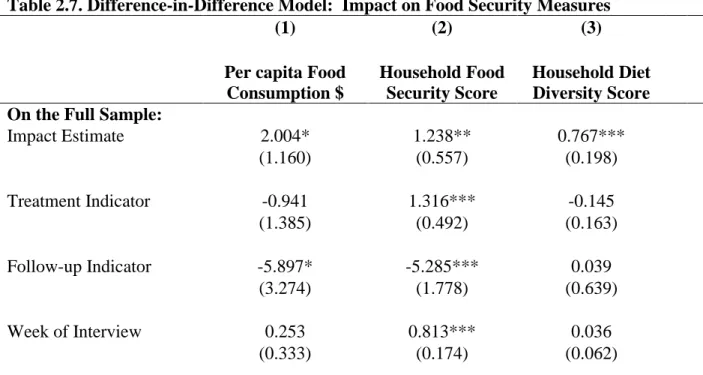
Table 2.7. Difference-in-Difference Model: Impact on Food Security Measures ... 38
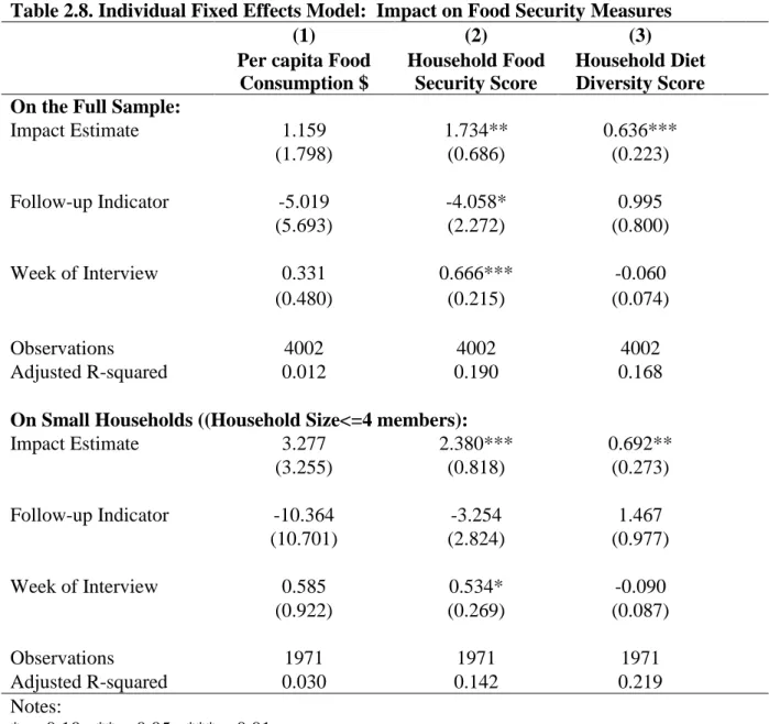
Table 2.8. Individual Fixed Effects Model: Impact on Food Security Measures ... 40
Table 2.9. Household Diet Diversity Impact Estimates ... 41
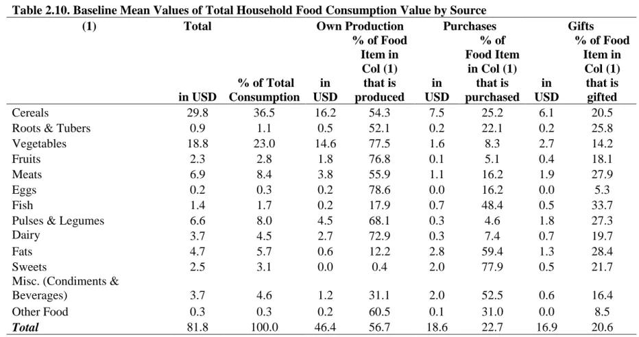
Table 2.10. Baseline Mean Values of Total Household Food Consumption Value by Source .... 43
Table 2.11. Impact Estimates on Household Food Expenditure, Disaggregated by Source ... 45
Table 3.1. Study Sample Size ... 68
Table 3.2. Household Level General Attrition ... 70
Table 3.3. Household Level Selective Attrition ... 71
Table 3.4. Baseline Mean Characteristics of Panel Sample Households ... 74
Table 3.5a. Average Satisfaction with Life Scores by Treatment and Comparison Groups ... 77
Table 3.5b. Average Value of Mediators across Treatment and Comparison Groups ... 81
Table 3.6. Baseline Determinants of Satisfaction with Life (Log of SWLS Score) ... 84
xii
Table 3.8. Impact Estimates of the Cash Transfer on Life Satisfaction and
Other Subjective Wellbeing Indicators: Individual Fixed Effects Model ... 97 Table 3.9. Impact Estimates of HSCT on Satisfaction With Life Score
Mediated through Food Insecurity ... 99 Table 3.10. Impact Estimates of HSCT on Satisfaction With Life Score
Mediated through Contributions ... 100 Table 3.11. Impact Estimates of HSCT on Satisfaction With Life Score
Mediated through Trust... 101 Table 3.12. Mediation Estimates: Fixed Effects ... 103 Table 3.13. Impact Estimates of HSCT on Satisfaction With Life Score:
Mediation Subsample Analyses ... 105 Table 3.14. Impact Estimates of HSCT on Satisfaction With Life Score
Mediated through Education Expenses ... 108 Table 4.1. Baseline Mean Characteristics of Panel Sample Households ... 128 Table 4.2. Means of Inter-Household Transfers and Related Outcomes
by Treatment and Comparison Groups ... 132 Table 4.3. Socioeconomic Variables Associated with Gifts
Received or Made (Baseline Sample) ... 136 Table 4.4. Impacts Estimates on Inter-Household Transfers and Related Outcomes ... 142 Table 4.5. Impacts Estimates on Inter-Household Transfers and Related Outcomes:
Subsample analyses ... 144 Table A.1. Full Results from Interacted Model Comparing
Pre/Initial Harvest vs. Peak Harvest ... 152 Table A.2. Difference-in-Difference Model: Impact of the Cash Transfer on
Food Security Measures (without controlling for week of interview) ... 154 Table B.1. Household Level Estimates of Differential Attrition ... 155 Table B.2. Baseline Mean Characteristics of Panel Households -
1
CHAPTER 1: INTRODUCTION
1.1 Research Objective
Cash transfers are increasingly being utilized as a preferred strategy for poverty alleviation. They refer to programs that provide direct cash to a targeted population group that fulfills specific eligibility criteria for receiving these transfers from the government. As such, this concept is as old as the welfare state: non-contributory pension schemes, disability benefits, child allowance and income support, student grants and scholarships, and assured work programs are all examples of direct cash transfers. However, reliance on cash transfers as the main vehicle of national social protection programs with poverty reduction as their main objective is relatively recent. These were first popularized in Latin America in the 1990s and have since then been embraced by several developing countries in Asia and Africa. Currently more than a hundred countries implement conditional or unconditional cash transfer programs (FAO, 2015). The theoretical basis for these programs is that regularity and predictability of cash payments allow poor households to smooth income and consumption across the year.
Cash transfer programs operate across all four categories of the asset-based social protection framework provided by Adato and Bassett (2008):
Protection - secure basic consumption needs
2
Promotional – help people to build their human, financial, and physical capital by enabling them to take-up educational and health services, access credit on better terms, and buy productive assets,
Transformational - build assets and make institutional changes that strengthen economic, political, and social relationships
Theory, therefore, tells us that social protection programs can have wide ranging effects on the entire household economy. Fiszbein and Schady (World Bank, 2009), Handa and Davis (2006), and Adato and Basset (2008) provide excellent overviews of the impact of different cash transfer programs on poverty, food consumption, schooling, health, asset accumulation,
economic productivity, and HIV prevention. Considerably less research however, has been conducted on impact of social cash transfers on experienced wellbeing of beneficiaries, the interplay between objective and subjective measures of wellbeing, and on understanding the underlying mechanisms that lie behind the impacts that we observe. My dissertation investigates non-obvious ways in which social programs can affect households such as resilience,
psychosocial wellbeing and social capital. There is scarce research on these nuanced, and potentially very important, but often ignored areas of wellbeing.
1.2. Overview
3
survey, conducted at baseline and 12-month follow-up. The household survey instrument is comprehensive covering demographic, social, economic, and psychological information, both at the household and individual level. The study design is such that it allows me to use a
difference-in-difference model to compare changes over time for the treatment and a matched comparison group.
Paper 1: The Effect of Cash Transfers and Household Vulnerability on Food security in Zimbabwe
In this paper, I investigate determinants of food security as measured by a well-known food security scale – the Household Food Insecurity Access Scale (HFIAS) – and as measured by value of household food consumption composed of own-production, market purchases and gifts received. I find that several dimensions of household vulnerability correlate more strongly with the food security measure than with food consumption. Labour constraints, which is a key vulnerability criterion used by the HSCT to target households, is an important predictor of the food security score but not food consumption, and its effect on food security is even larger during the lean season. Difference-in-differences impact analysis shows that the HSCT
4
Paper 2: Mediation Analysis of the Impact of an Unconditional Cash Transfer on
Subjective Wellbeing
This paper analyzes if an increase in income due to the cash transfer program increases the beneficiaries’ judgment of their overall life satisfaction (Direct Impact). To measure
subjective wellbeing I use the five-item Satisfaction with Life Scale that captures beneficiaries’ judgments of their overall life satisfaction. I find that the total impact of the cash transfer on Satisfaction with Life score is in the range of 14 to 17 percent. I next analyze if the impact of the cash transfer on overall life satisfaction is mediated through how people spend that income, i.e. through satisfaction of basic needs as indicated by decreased food insecurity and/or through satisfaction of higher-order needs as indicated by increase in social participation. I find that about 16 to 26 percent of the total impact is mediated through a reduction in food insecurity. Measures used to track social participation revealed only null to negligible mediation impact. Interviews with beneficiaries and key informants and focused group discussions reveal that the impact of the cash transfer on social participation is complex. While it can enable beneficiaries to be active participants in their communities, it can also lead to tension between beneficiaries and non-beneficiaries.
5
implicit role in sharing idiosyncratic risk. Empirical literature indicates that crowding-out can occur on the extensive margin, i.e. the probability of receiving a transfer, and on the intensive margin, i.e. amount of transfer conditional on it being positive. I therefore estimate - 1) the probability a household will receive informal transfers and 2) determinants of the monetary value of informal transfers. Utilizing a difference-in-differences methodology, I find that the program does not crowd-out informal inter-household transfers. Other mechanisms by which poor households manage risk and cope with liquidity constraints include contributions made to social networks or the ability to take out a loan. I do not find any impact of the Program on loans and amount outstanding of the beneficiary. However, number of households making contributions and the value of these contributions has increased, especially so for female-respondent
households. This suggests a type of ‘social re-engagement’ and an increased ability to participate in community life and ‘re-enter’ social networks. This is an important component of the
6
REFERENCES
Adato, M., & Bassett, L. (2008). What is the potential of cash transfers to strengthen families affected by HIV and AIDS? A review of the evidence on impacts and key policy debates. Boston, MA: Joint Learning Initiative on Children and AIDS.
Fiszbein, Ariel., Schady, Norber., Ferreira, Francisco H. G., Grosh, Margaret., Keleher, Niall., Olinto, Pedro., & Skoufias, Emmanuel. (2009). Conditional Cash Transfers: Reducing Present and Future Poverty. World Bank, Washington, DC. Retrieved from
https://openknowledge.worldbank.org/handle/10986/2597.
Handa, S., & Davis, B. (2006). The experience of conditional cash transfers in Latin America and the Caribbean. Development Policy Review, 24(5), 513–536.
7
CHAPTER 2: THE EFFECT OF CASH TRANSFERS AND HOUSEHOLD VULNERABILITY ON FOOD SECURITY IN ZIMBABWE
2.1.Introduction
The United Nations, as part of its post-2015 Sustainable Development Agenda, has declared ending hunger and achieving food security as the second of its 17-goal agenda, to be achieved by 2030. At present, about 795 million people are still undernourished globally, and the prevalence rate in sub-Saharan Africa is 23 per cent. In Zimbabwe, the proportion of
undernourished in the total population is even higher at 33 per cent (FAO, IFAD & WFP, 2015). In the past year, food security has worsened due to a poor 2015 harvest season and El Niño-induced below normal rains in early 2016. The Government declared a state of national disaster in February 2016 and appealed for USD 1.5 billion aid for food and other emergency needs. Dry and high-heat conditions have resulted in a significant reduction in cropped area and increased crop failure, particularly in the drought-affected southern districts (FEWS NET, March, 2016). Addressing the challenge of growing food insecurity requires implementation and scale up of effective social protection programmes.
8
down. We utilize longitudinal data from a large impact evaluation conducted as part of the second scale-up wave of the programme. Data was collected on 3063 households across 60 clusters in six districts. Households in 60 Wards were slotted to enter the programme immediately and serve as the treatment group for the evaluation, while households in the 30 Wards resided in areas that were to enter the programme in a later phase and thus serve as the comparison group.
To better understand food security we utilize baseline data to compare determinants of food security as measured by the Household Food Insecurity Access Scale (HFIAS) and the value of per capita food consumption within the household. The analysis indicates that factors, which directly reflect household vulnerability, such as exposure to shocks, labour constraints, and income from casual labour, are significant in explaining variation in the Food Security score but not food consumption. This provides evidence that a consumption-based measure may not fully capture household vulnerability. We extend the vulnerability analysis by stratifying our sample of baseline households into those that were interviewed just prior to the harvest season (and so presumably would be more food insecure) and those interviewed during the harvest season (and so would be less food insecure). We find that the negative impact of being labour constrained is accentuated during the lean phase, but only for the Food Security measure,
suggesting that the difference between the two measures is even more apparent when risk is high. This finding underlines the important practice of utilizing labour-constrained status as an
9
Utilizing a difference-in-differences methodology, we find that after 12 months of implementation, the Zimbabwe HSCT Programme has had a null to low impact on value of food consumption but statistically significant positive impacts on Food Security and Diet Diversity scores. A detailed analysis that disaggregates food consumption into consumption sourced from own-production, market purchases and gifts received, reveals that access to cash allowed households to purchase more food from the market, diversify its own-production of certain foodstuffs, and rely less on gifts as a source of food. Disaggregation of food consumption into different food groups also reveals that the cash allows households greater choice in their food basket. These changes are captured by the Food Security score and the Diet Diversity score but not in the value of aggregate food consumption.
This paper makes contributions to two distinct but inter-related literatures. First, we provide evidence on the relative merits of using a comprehensive consumption expenditure measure versus a food security scale to assess household vulnerability and food insecurity. While consumption is the preferred measure for economists, those working specifically in food security maintain that consumption alone does not pick up the multiple and nuanced dimensions of food security that go beyond access. Second, we contribute to a small but growing literature on the effects of state-sponsored unconditional cash transfers in Africa on household behavior and wellbeing. Existing evidence on cash transfers is dominated by studies from Latin America on conditional cash transfers, and many of those are from one single program
10 2.2. Literature Review
Food security is defined as the situation “when all people, at all times, have physical, social and economic access to sufficient, safe and nutritious food to meet their dietary needs and food preferences for an active and healthy life" (FAO, 2009). A common framework utilized by scholars to highlight the different dimensions of food security is a four-tier categorization – availability of food; access to food, which refers to the ability of households to obtain food from the market or own production or gifts; utilization of food; and stability, which is the ability of households to withstand risks and shocks that erode any of the other three dimensions (Webb et al., 2006).
During the 1980s, due in large part to the work of Sen (1981), there was a shift of emphasis from food-availability indicators to food-access indicators. Sen’s argument was that it is not enough if the country or region has adequate food supplies to feed its population, but the population also needs to have the ability to access this food. Another shift in focus has been in moving from objective to experiential measures. This change has been driven by the recognition of the experiential aspect of the process that leads to the condition of being hungry. Some
households can be food insecure, and yet not immediately experiencing hunger. The rationale for utilizing experiential-based indicators is that it “puts people’s experiences and behavioral
11
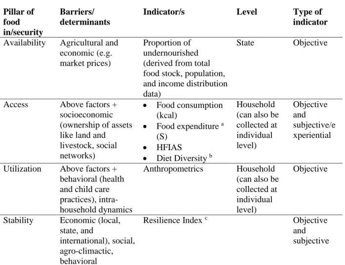
Table 2.1. Measures Corresponding to each pillar of Food security
Pillar of food in/security
Barriers/ determinants
Indicator/s Level Type of
indicator
Availability Agricultural and economic (e.g. market prices)
Proportion of undernourished (derived from total food stock, population, and income distribution data)
State Objective
Access Above factors + socioeconomic (ownership of assets like land and
livestock, social networks)
Food consumption (kcal)
Food expenditure a (S)
HFIAS
Diet Diversity b
Household (can also be collected at individual level) Objective and subjective/e xperiential
Utilization Above factors + behavioral (health and child care practices), intra-household dynamics
Anthropometrics Household (can also be collected at individual level)
Objective
Stability Economic (local, state, and
international), social, agro-climactic, behavioral
Resilience Index c Objective
and subjective
a Value of all food expenditure including value of gifts and own production consumed, divided by family
size
b Value of expenditure (including gifts and own production consumed) on eight different food groups:
cereal, roots and tubers, meat/poultry/fish, fruits and vegetables, pulses, dairy, sugar/fats, and food eaten out
c The Resilience Index indicator has only recently been conceptualized. It is yet to be operationalized and
therefore currently there are no indicators to satisfactorily measure the fourth pillar. This is because it is difficult to capture the dynamic aspect of food insecurity. Conceptually,
R = f(IFA = income and food access; ABS = access to basic services; AA = agricultural assets; NAA = non-agricultural assets; APT = agricultural practice and technology; SSN = social safety nets; CC = climate change; EIE = enabling institutional environment; S = sensitivity; AC = adaptive capacity)
12
primary objectives of cash transfer programmes. The theoretical basis for these programmes is that regularity and predictability of cash payments allow poor households to smooth
consumption across the year and build human and physical capital that will allow them to absorb shocks (Arnold et al., 2011; FAO, IFAD & WFP 2015). Their impacts on food consumption and nutrition have been well documented (Adato and Bassett, 2008; Kenya CT-OVC Evaluation Team 2012). According to a comprehensive review by the Department for International Development of the United Kingdom (Arnold et al., 2011), about half the value of the cash transfer is spent on food. However, impacts vary depending on the duration over which the transfer is received, age of the recipient, and size of the transfer. In Malawi, Miller et al. (2011) demonstrate large effect sizes that are statistically significant on food expenditure, consumption, and diet diversity. They also find upwards of a 32 percentage point (pp) difference in the
following four questions that capture food adequacy: do households consume less than enough; are they still hungry after meals; do they experience more than eight days per month without adequate food; are at least two meals consumed daily. These large effect sizes are explained in part by the size of the cash transfer, which ranged from $4.29 to $22 per month, and on average accounted for sixty percent of per capita total household expenditure.
In this paper we use a longitudinal ward-level matched case-control design to analyze the impact of a cash transfer programme implemented in rural Zimbabwe on household food security after 12 months of implementation. Within access-to-food measures we focus on value of
13
scale, with a reference period of the past four weeks where households are asked to rate their experience on a scale from ‘Rarely’ to ‘Often’, generating a total score from 0 to 27. It thus “provides a continuous measure of the degree of food insecurity of the household” (Coates, Swindale & Bilinsky, 2007, p.18). A higher score indicates the household suffers from more food insecurity and is relatively worse off. It captures the experiential aspect of food insecurity by including anxiety about future availability of food; consumption of food items that are not preferred; and limiting diet diversity as part of its construct. These three domains were identified based on the ethnographic work done by Radimer, Olson & Campbell (1990) in the United States. Coates et al. (2006) confirmed these domains to be common across diverse cultural settings.
The HFIAS then, goes beyond a food expenditure measure by capturing not just present food consumption status but also the uncertainty and vulnerability associated with maintaining or improving that status1. Vulnerability has been defined in different ways but the basic idea is that it is forward looking and captures the risk or “likelihood that at a given time in the future, an individual will have a level of welfare below some norm or benchmark” (Hoddinott and Quisumbing, 2003, p. 9). It is a forward-looking concept as opposed to a snapshot in time presented by food consumption expenditure. This distinction has been well documented in the literature on poverty (Dercon, 2001; Chaudhuri et al. 2002; Hoddinott and Quisumbing, 2003). In the food insecurity literature, the direction this research has taken has been generally that of validation studies. Jones et al. (2013) provide a review of four key validation studies of HFIAS in Iran (urban Tehran), Tanzania (poor rural households), Burkina Faso (urban households), and
1 Aside from construct validity, an additional reason why practitioners might choose to utilize the HFIAS
14
Ethiopia (community health volunteers). They find evidence of the construct validity of the HFIAS and high internal consistency. They also find that the HFIAS score is negatively
associated with other proximate determinants for food security such as household wealth/assets, maternal education, husband’s education, household per capita income and expenditure, and diet diversity. In Zimbabwe, Nyikahadzoi et al. (2013) found the HFIAS score to be higher in elderly headed households and within these households, food insecurity is negatively associated with social capital, remittances, and off-farm income. In another study among smallholder farmers in the Mudzi district of Zimbabwe, Mango et al. (2014) found that the HFIAS score is predicted by household labour, education of the household head, household size, remittances, livestock ownership and access to market information.
Migotto et al. (2005) compare a Consumption Adequacy Question (CAQ) with household caloric consumption, expenditure, diet diversity, and anthropometry in Albania, Indonesia, Madagascar and Nepal. They find that the CAQ is only weakly correlated with these indicators and that there is poor overlap among them in that they do not categorize the same households as food insecure. They assess if the CAQ is too subjective to make comparisons across households, perhaps because it captures relative food insecurity (relative to food status in the past and
relative to others in the community). They find that perception of food adequacy is highly correlated with subjective perceptions of future and past wealth, and thus may be capturing ‘vulnerability’, which the other quantitative indicators do not capture. However, they caveat their findings because statistical significance of subjective answers could simply be capturing
15
households in nine villages in Burkina Faso across five time periods from 2001-2003. They calculate a household food insecurity score from an HFIAS-like scale and find it to be negatively and significantly correlated with economic status (total assets and net income per adult
equivalent) and dietary intake indicators (such as food share expenditure) but not significantly correlated with anthropometric indicators. In another longitudinal study, Loopstra & Tarasuk (2013) find that changes in income and employment over the span of one year among 331 low-income families living on market-rent in Toronto are significantly associated with changes in severity of food insecurity.
2.3. Research Setting and Design
2.3.1. The Zimbabwe Harmonized Cash Transfer Program
We use data collected for the evaluation of the Harmonized Social Cash Transfer (HSCT) Programme, an unconditional cash transfer program, introduced in 2011 by the Government of Zimbabwe. Program implementation is being done in a phased manner and it is anticipated that eventually the Program will cover the entire country. In January 2016, the Program covered 52,500 households, and approximately 300,000 households are expected to be eligible for the program at full-scale.
Benefits are structured such that the size of the transfer varies with household size: a one-person household receives USD10, two-one-person receives USD15, three-one-person receives USD20, and a household made up of four or more persons receives USD25. The program thus provides between $10 and $25 per month, which represents about 20 percent of total household
16
The program is targeted at households that are food-poor and labor constrained. Eligible households are identified through a detailed targeting census that is conducted by ZIMSTAT, the national statistical agency. All households are screened using the targeting survey fielded by ZIMSTAT, and data is then processed to compute a proxy poverty score that serves as the first eligibility criterion. A household is considered food-poor when it is living below the food poverty line2 and is unable to meet the most basic needs of its members. A list of ten indicators
that measure the ability of the household to meet basic needs is used to determine eligibility on this criterion.3 At least three of these have to be met for the household to be eligible for the Program.
The Program has a clearly defined approach for categorizing a household as labor
constrained, which is the second eligibility criterion. Throughout the paper, we use this definition to operationalize the attribute of being labor constrained. A household is considered labor
constrained when:
1. There is no able bodied household member between 18-59 years who is fit for productive work, OR
2. The dependency ratio is three or more, i.e., one fit to work household member between 18-59 years has to take care of three or more dependents. Dependents are
2 Food poverty line is the threshold where total household expenditure is below what is required to meet
the food energy requirement for each household member, set at 2,100 kcal/day/person.
3 The 10 indicators as given in Form1R, which is used for assessing eligibility are: only one or no meals
17
those household members who cannot or should not work because they are under 18 years of age or they are elderly (over 59 years of age) or they are unfit for work because they are chronically ill or disabled or still in school, OR
3. The dependency ratio is between two and three and the household has a severely disabled or chronically sick household member who requires intensive care.
2.3.2. Study Design
The phased roll out of the HSCT allows us to use households in regions slotted to enter the program at a later date to form a comparison group. Within districts the program operates at an administrative unit known as the Ward. Child Protection Committees (CPCs) are formed within each Ward who are responsible for ensuring that targeting of households is conducted thoroughly and who are in charge of communication of program rules and operational activities (such as payment dates) between the district social welfare office and beneficiary households. The geographic area of a Ward varies by population density as each Ward comprises a cluster of anywhere from 10-20 villages. The Ward comprises the primary sampling unit for the sample design.
18
Harare. Each Ward was assigned a point score based on five characteristics: forest cover,
nearness to main roads, resistance to shocks, nearness to business centers, and water sources. On each criterion a Ward was scored from 1 (low) to 3 (high) and the maximum score possible was thus 15.4 Power calculations based on the expected number of households per Ward indicated that a total of 60 Treatment and 30 Comparison Wards were necessary for the study.5 The 60 treatment Wards were stratified across the three treatment districts (Mudzi, Mwenezi and Binga), and the 30 comparison Wards were likewise stratified to areas adjacent to the three treatment districts.
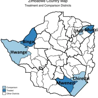
Wards in treatment areas were ranked from highest point score (most vulnerable) to lowest and paired with each stratum. Then, for each treatment Ward pair with a given score, a comparison Ward with the same score in the same stratum was selected to serve as the ‘matched’ comparison Ward. In cases where more than one comparison Ward existed with the same score, one was picked randomly. In cases where no comparison Ward existed with the exact same score, the Ward with the closest point score was selected. Figure 2.1 provides a map showing the geographic location within Zimbabwe of the study sites.
4 Details of the Ward level analysis are available upon request.
5 Sample size calculations were based on the power to detect a meaningful change in the height-for-age
19 Figure 2.1. Map of Zimbabwe
Source: Constructed using Stata 13.1. The darker outlines in the map are province boundaries. Shape files obtained from http://www.gadm.org/
20
out, it was concluded that overall attrition (households remaining in the study were no longer representative of households in the original sample) might be a problem (American Institutes for Research, 2014). To correct for this problem, inverse probability weighting was used to adjust sampling weights. We use these generated analytical weights for our panel data impact analysis.
Table 2.2. Study Sample Size
Treatment Comparison Total
2013 2,029 1,034 3,063
2014 1,748 882 2,630
Total 3,777 1,916 5,693
21 2.4. Household Characteristics and Food Security
2.4.1. Socioeconomic Characteristics associated with Food Security
We utilize Ordinary Least Squares (OLS) to understand if the HFIAS is capturing information about a household’s vulnerability that conventional food access measures, such as food consumption expenditure, are not able to detect. Theoretically, the HFIAS should inform us not just about a household’s food consumption status, but also about the anxiety it experienced to sustain that level of food consumption. For ease of comparison with other indicators we
positively code the HFIAS so that higher scores indicate better food security, and refer to it as Food Security.
Table 2.3 presents the results of the OLS analysis where our two measures of food security, the Food Security Score and Log of per capita Food Consumption Expenditure, are regressed on proximate determinants of food security using baseline data only. Since our two dependent variables are measured on different scales, we cannot directly compare coefficient estimates. However, we can compare the relative importance of factors in explaining variation in each measure. As expected, we find that the larger the household size, the lower the value of its per capita food consumption. However, the relationship between household size and the Food Security score is not significant. Female-headed households have on average about seven per cent lower value of per capita food consumption, and age of main respondent is significant across both measures, although the magnitude of the estimate is small. If the main respondent has attended school then the Food Security score is higher by 0.6 points and per capita food consumption value increases by eight percent.6
6 The main respondent is the person that is interviewed when we visit the household to conduct our
22
Table 2.3. Estimates of Socioeconomic Characteristics of Households Associated With Food Security Score and Per Capita Food Consumption Expenditure
(1) (2)
Food Security Score
Log Per Capita Food Consumption
$
Household Demographics: Estimate
Std.
Error Estimate
Std. Error Household Demographics:
Household Size (log) 0.263 0.969 -1.498*** 0.104
# Children under 5 -0.290 0.247 0.088*** 0.027
# Children 6-17 -0.421** 0.179 0.082*** 0.022
# Adults 18 - 59 -0.398 0.241 0.094*** 0.017
# Elderly (>60) -0.132 0.270 0.098*** 0.029
Main Respondent Characteristics:
Female (Yes=1) -0.419 0.292 -0.069** 0.031
Age (Years) -0.028*** 0.010 -0.002* 0.001
Widowed (Yes=1) -0.323 0.302 0.025 0.038
Divorced/Separated (Yes=1) 0.051 0.457 0.021 0.045
Main resp. has schooling (Yes=1) 0.601* 0.304 0.077** 0.032 Other socioeconomic Characteristics:
Distance to Food Market (Km) -0.077*** 0.025 0.001 0.002 Distance to Input Market (Km) 0.022*** 0.008 0.001 0.001 Distance to Water Source (Km) -0.016 0.118 -0.008 0.009
Productive Assets Scorea 0.507*** 0.089 0.074*** 0.008
Household Amenities Scoreb 0.528*** 0.106 0.051*** 0.010
# of livestock type 0.096 0.103 0.037*** 0.008
Any income from wage labor? (Yes=1) 1.530*** 0.462 0.151*** 0.040 Any income from maricho labor? (Yes=1) -0.787** 0.305 0.036 0.024 Planted crops last rainy season (Yes=1) 1.722*** 0.514 -0.008 0.044
Labor Constrained (Yes=1) -0.898** 0.386 -0.011 0.043
Aid received (in USD) -0.001 0.002 0.000 0.000
Monthly remittances low (< $25/month) -1.350** 0.518 -0.192*** 0.040 Has loan outstanding (Yes=1) -0.579 0.376 0.116** 0.045 Other covariates:
Suffered from a shock? (Yes=1) -1.975*** 0.402 0.000 0.036
Mashona Indicator -1.255*** 0.353 0.251*** 0.043
Masvingo Indicator -1.037** 0.447 0.255*** 0.036
Constant 19.010*** 1.448 4.766*** 0.134
23
Observations 3035 3035
Adjusted R-squared 0.130 0.467
Notes:
* p<0.1, ** p<0.05,*** p<0.01.
Standard errors clustered at the ward level. Standardized baseline weights utilized.
a Productive assets score obtained through Principal Components Analysis of 30 different
variables that indicate ownership of assets such as tractor, plough, and other agricultural tools and total land area of the household. Based on this analysis and the scree plot shown in Appendix A Figure A.1a, we retain the first principal component as our Productive Assets score for the household, which explains 21.5 per cent of the variability in the data. The subsequent components each explain less than six per cent of the variation.
b Household Amenities score also obtained through Principal Components Analysis of
variables that indicate ownership of the following amenities: a toilet, a cooking room, ventilation in the cooking room, access to energy for lighting within the house, household structure with more than two rooms, and sturdy walls made of bricks, stone or cement. Scree plot for this analysis is shown in Appendix A Figure A.1b. We retain the first component as the Amenities score for the household. It explains 31.3 per cent of the variation among the variables.
24
extremely poor households, or when the household suffers a shock or when grain stocks have run out and cash is needed. These results suggest that households smooth their consumption across time and their vulnerability in maintaining that consumption level is not immediately reflected in aggregate value of food consumption, but it is captured by the Food Security score.
2.4.2. Initial Harvest Period vs. Peak Harvest Period
We extend our vulnerability analysis by taking into account the fact that the baseline survey was implemented between April and June, so that some households were interviewed just prior to harvest and others during or just after. In an agrarian rural setting such as the one in which the HSCT was implemented, the time of the harvest can make a big difference to the food status of household members. Most rural households rely heavily on own-production of cereals, but also rely on the market, as own-production is not sufficient to meet their food requirements (FEWS NET, 2014).
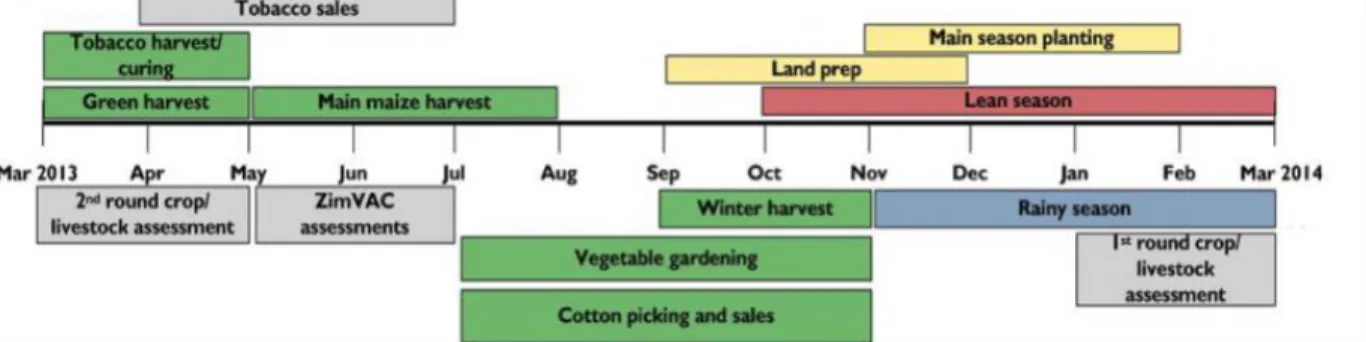
Figure 2.2 provides a graphic representation of Zimbabwe’s typical seasonal calendar. Zimbabwe has a unimodal rainy season lasting from November to March. This is also the main planting season of the year. Tobacco is the main cash crop of Zimbabwe and its harvest begins in March. The main maize harvest, which is the staple crop of the country, begins in May. The peak vegetable gardening and cotton-picking season then begins in July. Food insecurity starts
25 Figure 2.2. Zimbabwe Seasonal Calendar
Source: Famine Early Warning Systems Network
Figure 2.3 depicts how the Food Security score progresses across April-June, the survey window for 2013, and also the period when households are beginning to move out of the lean season to initial and then peak harvest period when they are typically flush with grains from own-production. Note that the food security score is based on a four-week reference period. Households interviewed in April/May were requested to think back to March/April, when they would have not yet entered the maize harvest period. As seen in Figure 2.3, there is a
26 Figure 2.3. Food Security score by Week
27
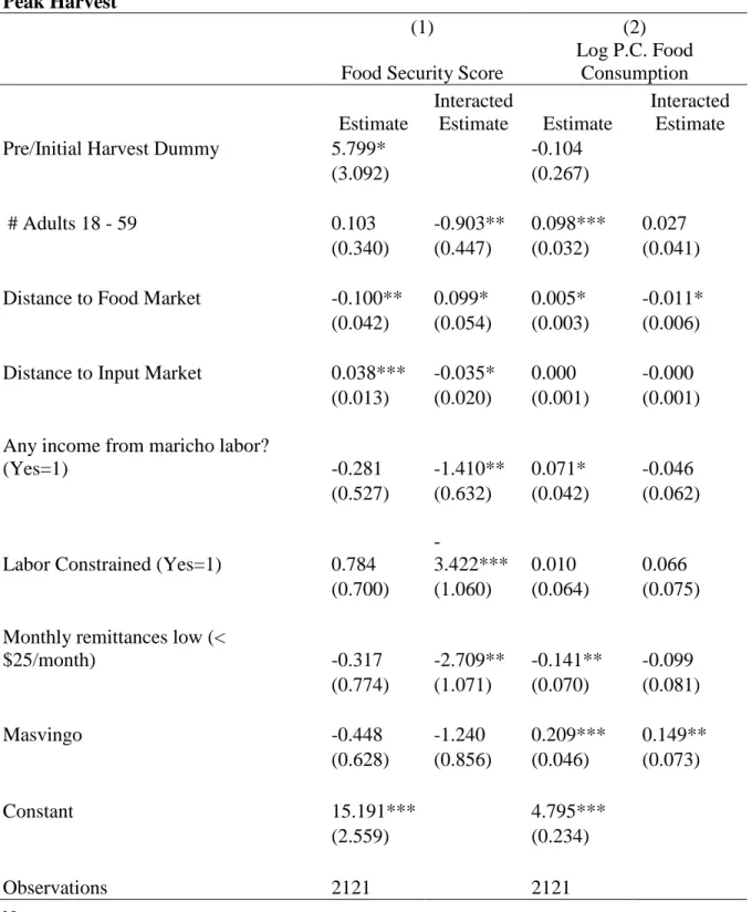
Table 2.4. Results from Fully Interacted Model Comparing Pre/Initial Harvest vs. Peak Harvest
(1) (2)
Food Security Score
Log P.C. Food Consumption Estimate
Interacted
Estimate Estimate
Interacted Estimate
Pre/Initial Harvest Dummy 5.799* -0.104
(3.092) (0.267)
# Adults 18 - 59 0.103 -0.903** 0.098*** 0.027
(0.340) (0.447) (0.032) (0.041) Distance to Food Market -0.100** 0.099* 0.005* -0.011*
(0.042) (0.054) (0.003) (0.006) Distance to Input Market 0.038*** -0.035* 0.000 -0.000
(0.013) (0.020) (0.001) (0.001) Any income from maricho labor?
(Yes=1) -0.281 -1.410** 0.071* -0.046
(0.527) (0.632) (0.042) (0.062)
Labor Constrained (Yes=1) 0.784
-3.422*** 0.010 0.066 (0.700) (1.060) (0.064) (0.075) Monthly remittances low (<
$25/month) -0.317 -2.709** -0.141** -0.099
(0.774) (1.071) (0.070) (0.081)
Masvingo -0.448 -1.240 0.209*** 0.149**
(0.628) (0.856) (0.046) (0.073)
Constant 15.191*** 4.795***
(2.559) (0.234)
Observations 2121 2121
Notes:
* p<0.1, ** p<0.05,*** p<0.01.
28
Maricho labour income increases food consumption during peak harvest but during
pre-harvest, it hurts the food security score of households. This suggests that households that engage in maricho labour in the pre-harvest period are poorer and are forced to rely on casual labour. Importantly, we find that if the household is labour constrained or receives low monthly
remittances, its food security is weakened in this period. Being labour constrained stands out as an especially vulnerability-inducing attribute. It is important to note that several social protection programmes throughout Africa – Ethiopia, Liberia, Malawi, Rwanda, Uganda and Zambia – utilize labour-constrained status as a targeting criterion for identifying programme beneficiaries.7
2.5. Impact of the HSCT Programme on Household Food Security 2.5.1. Summary Statistics
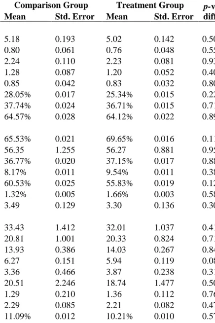
Table 2.5 reports mean characteristics at baseline for both treatment and comparison groups. We retain only the panel sample of households for this part of our analysis. There are 1,746 households in the treatment group and 880 in the comparison group. To test for baseline balance between the two groups, we use OLS regressions with clustered standard errors at the ward level (to account for clustering of households within wards). Mean differences in a set of 30 key household characteristics were tested, and none of these were found to be statistically different at the five per cent level at baseline.
Average household size in the sample is about five, with a per capita monthly
expenditure of $32-33. More than two-thirds of the main respondents are women, their average
7 Some programme names include the Malawi Social Cash Transfer Programme, the Kenya Cash Transfer
29
age is 56 years, and more than half have had at least some level of schooling. Around 25-28 percent of these households take care of one or more disabled members. In addition, around 37 percent have at least one member who is chronically ill and almost two-thirds have one or more elderly members. These characteristics contribute to a high dependency ratio, which is reflected in the large number of households that are categorized as labor constrained (about 83-84 percent of the sample8). That our sample should have such a high concentration of labor-constrained households makes sense because as mentioned earlier, one of the program criterions for household eligibility is labor-constrained status of the household. This demographic profile is also reflected in the unique U shape of the age distribution among HSCT households shown in Figure A.2 of Appendix A. There are a large proportion of young people (almost 60 per cent of individuals in our sample are below 18 years of age, and most are adolescents), a few working-age adults, and then the distribution again expands to indicate a higher concentration of people beyond age 60. This profile reflects the ‘missing generation’ problem characterizing much of sub-Saharan Africa, wherein older caregivers are providing for adolescents, because prime-age, able-bodied workers are ‘missing’, due to high mortality rates induced by high HIV/AIDS prevalence rates. The addition of the labour-constrained criterion in addition to food poverty is important because it led to the selection of socially vulnerable households.
Table 2.6a provides means of food security measures across our two time periods. A higher Food Security score indicates the household has higher food security and is relatively better off. Cronbach’s alpha for the food security scale in the two time periods is 0.86 at baseline and 0.87 at follow-up, suggesting that the sub items of the scale have relatively high internal
8 The reason this is not hundred percent is because the questions used to determine labour constraint are
30
consistency.9,10 The average Food Security score increased from 13 at baseline to above 16 at follow-up, a pattern that holds for both treatment and comparison groups. This improvement is because the baseline survey window began in the pre-harvest season (April-June 2013) while the follow-up survey in 2014 was conducted entirely during peak harvest time (June-September 2014) when households are generally flush with food supplies.
Value of average household food consumption per person per month has decreased by a dollar for the treatment group and almost two dollars for the comparison group. Kernel densities of the Food Security score and log of per capita monthly food consumption are provided in Figure A.3 of Appendix A.
A widely used indicator of diet diversity is the Diet Diversity Score (DDS), which measures the number of different food groups consumed over a given reference period with a score ranging from 0 to 12, since there are 12 food groups11 recommended for inclusion
9The nine sub-items of the scale items are: 1) did you worry that your household would not have enough
food?, 2) were you or any household member not able to eat the kinds of food you preferred because of a lack of resources?, 3) did you or any household member have to eat a limited variety of foods due to a lack of resources?, 4) did you or any household member have to eat some foods that you really did not want to eat because of a lack of resources to obtain other types of food?, 5) did you or any household member have to eat a smaller meal than you felt you needed because there was not enough food?, 6) did you or any household member have to eat fewer meals in a day because there was not enough food?, 7) was there ever no food to eat of any kind in your household because of lack of resources to get food?, 8) did you or any household member go to sleep at night hungry because there was not enough food?, and 9) did you or any household member go a whole day and night without eating anything because there was not enough food?
10 Cronbach's alpha is a measure of internal consistency and is used as a measure of scale reliability. It
measures how closely related a set of items are as a group. Generally, a coefficient of 0.80 or higher is considered acceptable for conducting research.
11 The 12 food groups are: Cereals; Roots and Tubers; Vegetables; Fruits; Meat/Poultry; Eggs;
31
(Swindale & Bilinsky, 2006). Average household diet diversity based on this score increased from about 6 at baseline to 6.76 for the comparison group and 7.16 for the treatment group.
Table 2.6b provides a correlation matrix of standard pairwise Pearson’s Correlation coefficients using 2013 (baseline) data only. Correlations are in the expected direction but are low (correlation of Food Security score with per capita food consumption expenditure is only 13.6 per cent), suggesting, as we discussed in the previous section, that they are measuring different dimensions. Past empirical studies have also found low correlations between
Table 2.5. Mean Baseline Characteristics of Sample Households
Comparison Group Treatment Group p-value of difference
Mean Std. Error Mean Std. Error
Household Demographics:
Household Size 5.18 0.193 5.02 0.142 0.504
# Children under 5 0.80 0.061 0.76 0.048 0.550
# Children 6-17 2.24 0.110 2.23 0.081 0.931
# Adults 18 - 59 1.28 0.087 1.20 0.052 0.407
# Elderly (>60) 0.85 0.042 0.83 0.032 0.801
% of households that have disabled members 28.05% 0.017 25.34% 0.015 0.222 % of households that have chronically ill members 37.74% 0.024 36.71% 0.015 0.712 % of households that have elderly members 64.57% 0.028 64.12% 0.022 0.894 Main Respondent Characteristics:
% Female 65.53% 0.021 69.65% 0.016 0.116
Age (Yrs.) 56.35 1.255 56.27 0.881 0.951
% Widowed 36.77% 0.020 37.15% 0.017 0.883
% Divorced/Separated 8.17% 0.011 9.54% 0.011 0.389
% Main resp. has schooling 60.53% 0.025 55.83% 0.019 0.129
% Main resp. currently attends school 1.32% 0.005 1.66% 0.003 0.586
Highest grade of Main resp. 3.49 0.129 3.30 0.136 0.307
Other Socioeconomic Characteristics:
Monthly Per Capita Total Expenditure (in usd) 33.43 1.412 32.01 1.037 0.418 Monthly Per capita Food Expenditure (in usd) 20.81 1.001 20.33 0.824 0.714
HFIAS Score (1-27) 13.93 0.386 14.03 0.267 0.841
Diet Diversity Score (1-10) 6.27 0.151 5.94 0.119 0.089
Distance to Food Market (Km) 3.36 0.466 3.87 0.238 0.316
Distance to Input Market (Km) 20.51 2.246 18.74 1.477 0.508
Distance to Water Source (Km) 1.29 0.210 1.36 0.112 0.760
# of livestock type 2.29 0.085 2.21 0.082 0.477
% households that receive wages 11.09% 0.012 10.21% 0.010 0.575
% households undertaking casual/maricho labor 48.87% 0.034 46.20% 0.022 0.513 % households that planted crops last season 86.89% 0.026 90.11% 0.009 0.247 % households categorized as labor constrained 82.91% 0.020 83.97% 0.012 0.647
Aid received (in USD) 77.67 14.210 54.35 3.445 0.111
% of households that have an outstanding loan 8.85% 0.008 9.37% 0.013 0.741 % of households that have suffered from a shock 86.87% 0.020 90.04% 0.013 0.190 Notes: Attrition-adjusted weighted results, p-values obtained by clustering at ward
level
Table 2.6a. Mean of Food Security Measures
Comparison Treatment p-value
baseline difference
Baseline Follow-up Baseline Follow-up
Food Security Score 13.07 16.34 12.98 16.46 0.841
P.C. Food Consumption $ per month 20.81 19.09 20.33 19.33 0.714
Diet Diversity Score 6.27 6.76 5.94 7.16 0.089
N 879 880 1742 1743
Notes: Attrition-adjusted weighted results, p-values is of baseline difference between the two groups and obtained by clustering at ward level
Table 2.6b. Correlation Matrix of Food Security Measures using Baseline Data
Food Security Score
P.C. Food Consumption $ per month
Diet Diversity Score
Food Security Score 1
P.C. Food Consumption $ per month 0.1361 1
Diet Diversity Score 0.2604 0.3482 1
Notes: Attrition-adjusted weighted results
34 2.5.2. Empirical Methods
We utilize the longitudinal sample (containing two time periods, baseline and follow-up) to conduct a difference-in-differences (DD) analysis to estimate the impact of the programme on food security.
Equation (1):
𝑌ℎ𝑗𝑡 = β0+ β1Post𝑡+ β2Transfer𝑗+ β3(Transfer ∗ Post)𝑗𝑡
+ β4HHDemographicsℎ+ β5HHMainRespℎ+ β6Strata𝑗+ β7Prices𝑗𝑡
+ β8Week𝑡+ εℎ𝑗𝑡
where
Yhjtis the food security outcome of interest for household h in Ward j at time t. Postt is an indicator that equals ‘1’ if the time period is 2014 (12 month follow-up).
Transferj is an indicator that equals ‘1’ if the household is in a treatment Ward.
HHDemographics is a vector of baseline household demographic characteristics, which include log of household size, and the number of people below age 5, between age 6-17, between age 18-60, and those over 60.
HHMainResp is a vector of characteristics of the main respondent that includes indicators for if the main respondent is female, widowed, divorced/separated, has attended school, currently attends school, and linear variables for the highest grade attained and age.
Strata are indicators of the strata used in selecting Wards. It includes two dummies to indicate if the household was located in Mashonaland East or Masvingo. The
35
Pricesjt refer to a vector of cluster-level prices of eight staple items.
Weekt is the week in which the household is interviewed.
In this framework the variable of interest is β3, which represents the DD programme impact. Estimation is via Ordinary Least Squares (OLS) with standard errors clustered at the level of the primary sampling unit (Ward). We use baseline values for main respondent characteristics and household demographics, while prices are maintained as exogenous and allowed to vary by time period. We tested separately to see if the programme had an inflationary effect in treatment wards and found none, a plausible finding given that the overall coverage of the programme is only 10-15 per cent in the ward.
As described earlier, the study design is a ward level longitudinal matched design where households in both comparison and treatment districts went through official program targeting. Participation in the program is not demand-driven: the program eligibility identification process determines eligibility, and there were no refusals to participate in the program among eligible households, i.e., take up is universal among the eligible. The likelihood for selection bias in this context is minimal.
36
maintain the validity of this assumption. In addition, baseline balance tests indicate that households across the treatment and comparison samples are balanced on a number of key demographic and socioeconomic characteristics (see Table 2.5). This is as expected since all households are eligible for the HSCT, having been selected according to the same program eligibility criteria. This further supports the validity of the key identifying assumption.
The DD model does not control for differences between the treatment and comparison groups on account of household or individual unobserved characteristics. Our impact estimate (β3 in the above equation) may be biased if there are unobserved characteristics influencing both
the program and our outcome measure. A fixed effects model at the household level can address the issue of unobserved characteristics that are fixed over time as a source for endogeneity, and is therefore our preferred model:
Equation (2):
𝑌ℎ𝑗𝑡 = αℎ+ β1Post𝑡+ β2Transfer𝑗∗ Post𝑡+ β3Prices𝑗𝑡+ β4Week𝑡+ νℎ𝑗𝑡
where
Yhjt is the food security outcome of interest for household h in Ward j at time t.
αh (h=1….H) is the intercept for each household (h household-specific intercepts).
Post, Prices, and Week are as described in Equation (1).
β2 represents the impact estimate and νht is the time-varying error term.
37
Note that the threat unobservable characteristics impose to the validity of our model is minimal because, as mentioned above, households in both arms are selected according to program rules and take up is universal among the eligible, so there is no self-selection into the treatment group. There is a second reason, however, why employing the fixed effects model is warranted for estimating the impact on the Food Security score. Subjective or experiential measures can lead to responder bias since some element of their predisposition or attitudinal characteristics will enter into the responses they give for the set of nine questions that comprise the food security scale. It is, therefore, important to have panel data, where we follow the same respondent from one year to the next to control for this type of responder bias. We estimate Equation (2) using only the subsample of households where the main respondent has not changed from baseline to follow-up. Out of the 2,630 households that comprise our panel sample, over 76 percent (2,007 households) have the same main respondent across the two time periods.
2.5.3. Results and Discussion
Table 2.7 provides the results of our difference-in-differences model. Given the
importance of the week in which the households were interviewed, our difference-in-differences estimates control for week of interview, in addition to the standard set of baseline household demographics and main respondent characteristics, and contemporaneous prices.1 Results using the full panel sample are shown in first half of Table 2.7. We find that per capita food
consumption increased by $2 per month, which represents a ten per cent increase over baseline value of food consumption. As per the design of the programme, a household size of five (the median household size in our sample) receives $5 per person, so a $2 increase in food
1 Table A.2 in Appendix A shows the results of the Difference-in-Difference estimates on the full sample
38
consumption represents forty percent of the transfer dollars the household receives. In addition, we find a statistically significant impact on Food Security and Diet Diversity scores, which have increased by 1.2 points and 0.77 points.
The HSCT programme is designed so that per capita transfer size decreases with household size. However, the transfer size increases proportionally with household members only up to a point (four members) and then remains flat at USD25 for all households greater than four members. Since the median household size in our sample is five, over 50 per cent of
households have more than four members. To account for this variation in the intensity of the treatment, we restrict our sample to households with four or fewer residents (bottom panel of Table 2.7). In this case, we do not find a statistically significant average treatment effect on food consumption value or on the Food Security score. The magnitude of the impact on food
consumption has more than doubled to $4.4, but the t-statistic (1.6) is below the critical threshold.
Table 2.7. Difference-in-Difference Model: Impact on Food Security Measures
(1) (2) (3)
Per capita Food Consumption $
Household Food Security Score
Household Diet Diversity Score On the Full Sample:
Impact Estimate 2.004* 1.238** 0.767***
(1.160) (0.557) (0.198)
Treatment Indicator -0.941 1.316*** -0.145
(1.385) (0.492) (0.163)
Follow-up Indicator -5.897* -5.285*** 0.039
(3.274) (1.778) (0.639)
Week of Interview 0.253 0.813*** 0.036
39
Observations 5245 5245 5245
Adjusted R-squared 0.323 0.119 0.191
On Small Households ((Household Size<=4 members):
Impact Estimate 4.397 0.972 0.802***
(2.722) (0.697) (0.258)
Treatment Indicator -1.929 0.242 -0.359
(2.321) (0.589) (0.226)
Follow-up Indicator -11.113 -1.376 0.878
(6.783) (2.225) (0.884)
Week of Interview 0.365 0.391* -0.042
(0.639) (0.215) (0.088)
Observations 2355 2355 2355
Adjusted R-squared 0.231 0.088 0.215
Notes:
* p<0.10 **p<0.05 ***p<0.01
Standard errors clustered at the Ward level in parentheses.
Estimations use difference-in-difference modeling among panel households. All estimations control for baseline household size, main respondent’s gender, age, education and marital status, strata, household demographic composition, and a vector of cluster level prices.
To control for attitudinal bias in the Food Security score, we restricted the sample to only those households where the main respondent had not changed from 2013 to 2014 and run an individual fixed effects model, which controls for personality traits and other unobserved
40
Table 2.8. Individual Fixed Effects Model: Impact on Food Security Measures
(1) (2) (3)
Per capita Food Consumption $
Household Food Security Score
Household Diet Diversity Score On the Full Sample:
Impact Estimate 1.159 1.734** 0.636***
(1.798) (0.686) (0.223)
Follow-up Indicator -5.019 -4.058* 0.995
(5.693) (2.272) (0.800)
Week of Interview 0.331 0.666*** -0.060
(0.480) (0.215) (0.074)
Observations 4002 4002 4002
Adjusted R-squared 0.012 0.190 0.168
On Small Households ((Household Size<=4 members):
Impact Estimate 3.277 2.380*** 0.692**
(3.255) (0.818) (0.273)
Follow-up Indicator -10.364 -3.254 1.467
(10.701) (2.824) (0.977)
Week of Interview 0.585 0.534* -0.090
(0.922) (0.269) (0.087)
Observations 1971 1971 1971
Adjusted R-squared 0.030 0.142 0.219
Notes:
* p<0.10 **p<0.05 ***p<0.01
Standard errors clustered at the Ward level in parentheses.
Estimations control for week of interview, and a vector of cluster level prices
41
6pp for miscellaneous items, which include non-alcoholic beverages and condiments. Why are these increases not consistently reflected in the food consumption measure? One answer is that the value of food consumption variable hides dynamic activity that is taking place within the household as it makes choices to obtain food from different sources. This means that even though the treatment and comparison groups may on average spend roughly the same amount on food, the cash transfer beneficiaries have more cash available. This additional cash allows them to: 1) approach the market to diversify their food basket; 2) diversify own-production to other foodstuffs, and; 3) rely less on gifts as a source for their food.
Table 2.9. Household Diet Diversity Impact Estimates
Impact
Estimate Baseline Mean
Diet Diversity Score 0.767*** 6.045407
(0.198)
Presence of Food Item in Diet
Impact Estimate
Baseline Mean (%)
(1) Cereals -0.001 99.9
(0.001)
(2) Roots & Tubers 0.033 11.3
(0.051)
(3) Vegetables 0.002 98.9
(0.007)
(4) Fruits 0.126** 33.4
(0.056)
(5) Meats 0.005 38.8
(0.039)
(6) Eggs -0.038* 6.8
(0.020)
(7) Fish 0.016 22.6
(0.037)
(8) Pulses & Legumes 0.161*** 57.5
(0.044)
(9) Dairy 0.123*** 31.8
42
(10) Fats 0.147*** 64.1
(0.046)
(11) Sweets 0.134*** 46.9
(0.035)
(12) Misc. (Condiments & Beverages) 0.060*** 92.5 (0.020)
No. Of Observations 5245 2622
Notes: * p<0.10 **p<0.05 ***p<0.01
Standard errors clustered at the Ward level in parentheses
Notes: Attrition-adjusted weighted results. Estimations use
difference-in-difference modeling among panel households. All estimations control for week of interview, baseline household size, main respondent’s gender, age, education and marital status, strata, household demographic composition, and a vector of cluster level prices.
Table 2.10 provides baseline mean value of consumption for each of the 12 categories that make up the Diet Diversity score and disaggregated by source into own production, market purchases, and gifts. Since these households are subsistence farmers, own production is the primary source of food (~57 per cent), followed by purchases (~23 per cent), and a non-negligible amount (~21 per cent) of food is sourced from gifts (last column of Table 2.10). Cereal (in particular maize) is the staple food and accounts for 36.5 per cent of total food consumption value, followed by vegetables (23 per cent), meats (8.4 per cent) and pulses and legumes (eight per cent). Vegetables, fruits, eggs, and dairy are mostly own-produced. Over half of the cereal, roots and tubers, meat, and pulses consumption expenditure are from