An MRI segmentation framework for brains with anatomical deviations

(1)

An MRI Segmentation Framework for Brains with Anatomical

Deviations

Marcelinus Prastawa

A dissertation submitted to the faculty of the University of North Carolina at Chapel Hill in partial fulfillment of the requirements for the degree of Doctor of Philosophy in the Department of Computer Science.

Chapel Hill 2007

Approved by:

Guido Gerig, Ph.D.

Stephen R. Aylward, Ph.D.

Elizabeth Bullitt, M.D.

Sarang C. Joshi, D.Sc.

J. Stephen Marron, Ph.D.

(2)

c 2007

(3)

ABSTRACT

MARCELINUS PRASTAWA: An MRI Segmentation Framework for Brains with Anatomical Deviations

(Under the direction of Guido Gerig, Ph.D.)

The segmentation of brain Magnetic Resonance (MR) images, where the brain is partitioned into anatomical regions of interest, is a notoriously difficult problem when the underlying brain structures are influenced by pathology or are undergoing rapid development. This dissertation proposes a new automatic segmentation method for brain MRI that makes use of a model of a homogeneous population to detect anatomical deviations. The chosen population model is abrain atlascreated by averaging a set of MR images and the corresponding segmentations. The segmentation method is an integration of robust parameter estimation techniques and the Expectation-Maximization algorithm. In clinical applications, the segmentation of brains with anatomical deviations from those commonly observed within a homogeneous population is of particular interest. One example is provided by brain tumors, since delineation of the tumor and of any surrounding edema is often critical for treatment planning. A second example is provided by the dynamic brain changes that occur in newborns, since study of these changes may generate insights into regional growth trajectories and maturation patterns. Brain tumor and edema can be considered as anatomical deviations from a healthy adult population, whereas the rapid growth of newborn brains can be considered as an anatomical deviation from a population of fully developed infant brains.

A fundamental task associated with image segmentation is the validation of segmen-tation accuracy. In cases in which the brain deviates from standard anatomy, validation is often an ill-defined task since there is no knowledge of the ground truth (information

(4)

(5)

ACKNOWLEDGEMENTS

This dissertation was made possible through the active contributions of many people. In particular, I would like to thank my advisor Guido Gerig for providing refreshing guidance throughout my studies and for his continual support. I also want to thank my committee members: Dr. Elizabeth Bullit for her clinical expertise, for providing her extensive MRI data, and for funding my studies; Dr. Stephen Pizer for his guidance on all things related to medical image analysis; Dr. Sarang Joshi for his expertise in computational anatomy and for providing interesting research directions; Dr. Stephen Aylward for his expertise in medical image analysis, and for introducing me to the Insight Toolkit (ITK); Dr. Stephen Marron for his expertise in statistics, and for providing a clear education on many essential statistical concepts.

I would like to thank my fellow students in the Medical Image Display and Analysis Group (MIDAG), particularly Dr. Sean Ho, Dr. Peter Lorenzen, Nathan Moon, and many others. I am also grateful to the faculty and staff of the Computer Science depart-ment for providing a well-maintained, comfortable environdepart-ment for study and research. I particularly would like to thank Janet Jones for her help with all the administrative issues.

By its nature, medical image analysis is a multidisciplinary field and I am grateful for the opportunity to collaborate with the clinical researchers at UNC. I thank Dr. Weili Lin for providing the MR images, and Dr. John Gilmore for providing the opportunity to work on the newborn MRI data. I would also like to thank Dr. Martin Styner, Sylvain Gouttard, and Sampath Vetsa for providing useful feedbacks on my segmentation software.

(6)

The funding for the work described in this dissertation was generously provided by the National Institutes of Health (NIH). Particularly, through the grants NIBIB R01 EB000219, NCI R01 HL69808, and NIMH Conte Center MH064065. The UNC Schizophrenia Research Center and the UNC Neurodevelopmental Disorders Research Center (HD 03110) also provided other sources of funding.

(7)

LIST OF TABLES

3.1. Volumes of the manually segmented tumor and edema . . . 42

3.2. Intra-rater variability of manual tumor segmentation . . . 43

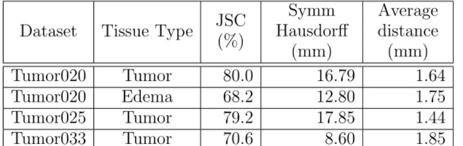
3.3. Validation measures of the automatic tumor segmentation results . . . 43

4.1. Newborn brain structure volumes. . . 62

4.2. Variability of the newborn brain MRI segmentations . . . 62

4.3. Volume overlap of two manual newborn brain MRI segmentations . . . 62

4.4. Volume overlap of the first set of manual segmentations and automatic results for newborn brains . . . 62

4.5. Volume overlap of the second set of manual segmentations and automatic results for newborn brains . . . 63

5.1. Volumes of the tumor and edema structures in the synthetic datasets . . . 96

5.2. Synthetic ground truth compared to manually drawn segmentations . . . 96

(11)

LIST OF FIGURES

1.1. A typical manual segmentation . . . 2

1.2. The ICBM brain atlas . . . 3

1.3. MR images exhibiting deviations . . . 4

1.4. Failed tumor segmentation . . . 5

1.5. Overview of dissertation topic . . . 6

2.1. A C-step iteration . . . 20

2.2. Minimum Spanning Tree clustering . . . 21

2.3. Low breakdown point for Minimum Spanning Tree clustering . . . 22

3.1. The three major stages of the brain tumor MRI segmentation method. . . 30

3.2. Model of the healthy adult population . . . 31

3.3. Example healthy adult MRI dataset . . . 32

3.4. Application of MCD to white matter training data . . . 33

3.5. First stage of brain tumor MRI segmentation . . . 35

3.6. Iterative density estimation for the abnormal class label . . . 35

3.7. T2-weighted image of the Tumor020 dataset . . . 37

3.8. Reclassification of brain tumor MRI using geometric and spatial properties . . 40

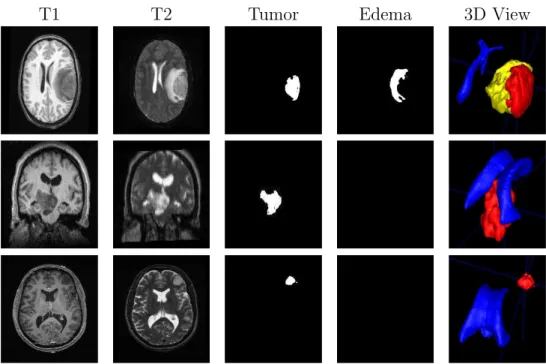
3.9. Visualization of the tumor segmentation results . . . 42

4.1. MRI of a newborn brain . . . 46

4.2. Intensity characteristics of a newborn brain MRI . . . 49

4.3. The probabilistic brain atlas of a newborn brain . . . 50

4.4. The segmentation framework for newborn brain MRI. . . 51

4.5. MST with and without gradient-constrained sampling . . . 53

4.6. Newborn brain MR images and the manual segmentations . . . 60

4.7. Surface renderings of the segmented structures of newborn subject 0123 . . . 61

(12)

4.8. Automatic segmentation results of newborn brain MRI . . . 61

4.9. Regional growth of cortical gray matter in newborns . . . 65

4.10. Regional growth of cortical unmyelinated white matter in newborns . . . 65

5.1. Overview of the generation of synthetic brain tumor MRI . . . 69

5.2. Tumor and edema growth model . . . 71

5.3. BrainWeb data . . . 72

5.4. Diffusion tensor MRI before and after tumor mass effect simulation . . . 79

5.5. Generation of contrast enhanced T1-weighted image . . . 83

5.6. Simulated probabilities related to contrast enhancement . . . 86

5.7. Real and synthetic contrast enhanced T1w MRI . . . 87

5.8. TSVQ using binary tree . . . 88

5.9. Synthetic brain tumor MRI compared to real MRI: SimTumor001 dataset . . . 91

5.10. Axial view of the synthetic brain tumor MRI datasets . . . 92

5.11. Coronal views of the synthetic brain tumor MRI datasets . . . 93

5.12. Axial views of the synthetic brain tumor MRI ground truth . . . 94

5.13. Coronal views of the synthetic brain tumor MRI ground truth . . . 95

5.14. Summary of the generation of synthetic brain tumor datasets . . . 99

(13)

CHAPTER 1

Introduction

1.1. Motivation

Medical image segmentation is the task of classifying image components (pixels or voxels) into relevant anatomical components or describing the structural and intensity changes in terms of the underlying functional process. The knowledge of the location, size, and shape of different anatomical structures is a fundamental step in understanding and analyzing medical images. Explicit knowledge of the segmented structures in med-ical images allows us to do more than qualitative visual assessment, as in the following examples:

• The location of a pathology relative to healthy anatomical structures is useful

in planning radiological treatments and surgeries.

• Growth patterns can be determined by analyzing changes of segmented

struc-tures of a population group over time.

• Analysis of the shape of the segmented brain structures can be used to find

characteristics or markers of neurological disorders.

(14)

Figure 1.1. Gadolinium contrast enhanced T1-weighted MR image (sagittal view) and the manual segmentation result. Note the ragged out-line in the segmentation that can be attributed to the slice-by-slice 2D painting in the axial direction (Tumor031 dataset).

generally time consuming and challenging. Furthermore, manual segmentations are dif-ficult to reproduce in a reliable and objective manner, even by the same human expert. The task is mostly performed by drawing image regions slice-by-slice, limiting the human rater’s view and generating suboptimal outlines with limited consistency across slices. An example of a manual segmentation of brain tumor from MRI is shown in Figure 1.1.

Due to the limitations of manual segmentation methods, an automatic segmentation framework is crucial for the study of medical phenomena, especially when it involves a large set of images. An automatic segmentation method is desirable because it reduces the work load of human experts and generates fully reproducible segmentations. A computer program also has the advantage of being able to process large amounts of information as typically presented within 3D multi-modal MR images in a more consistent manner compared to human raters.

1.2. Automatic MRI Segmentation

(15)

Figure 1.2. The ICBM (International Consortium of Brain Mapping) brain atlas that functions as a spatial probabilistic model for a healthy adult population. From left to right: T1 weighted template image and probability values of white matter, gray matter, and csf.

(information transmitters), gray matter (information processors), and cerebrospinal fluid. The central gray matter region can be divided further into other structures such as the caudate, hippocampus, etc. [37]. A widely used model for the general adult brain population is the probabilistic brain atlas [20], which is created by averaging MR images and the corresponding sets of segmentations. The ICBM (International Consortium of Brain Mapping) brain atlas (Figure 1.2) provides the spatial probabilities of a brain location being white matter, gray matter, or cerebrospinal fluid (csf). The atlas was created by registering subject images using affine transformation. Due to the limited degrees of freedom for affine transformation, most of the subject variability is retained and the atlas appears blurry. A sharper atlas can be created by using a deformable registration with more degrees of freedom, such as the fluid image warping [55]. A mesh-based atlas generation scheme that automatically determines the degree of warping and blurring was proposed by van Leemput [94].

Existing automatic MRI segmentation methods make use of the brain atlas as spatial priors [93] or as sampling constraints [17]. These methods provide good results for healthy brain MR images that have similar structure to the one described by the brain atlas. In clinical applications however, there is strong interest in analysis of MR images that show deviations from the typical population, which implies deviations from the reference population model (brain atlas). These deviations can be caused by pathology or natural growth patterns, as shown in Figure 1.3. The standard atlas-based segmentation methods fail in detecting anatomical deviations because they typically do not take into

(16)

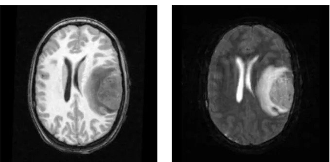
Figure 1.3. Example MR images that exhibit deviations from a reference population. Top: MRI of an adult with tumor and edema (T1w and T2w) which show deformation due to tumor mass effect and infiltration of brain tissue by edema. Bottom: MRI of a newborn infant (T1w and T2w) which shows the presence of two different types of white matter due to myelina-tion.

account strucutural and intensity changes not modelled by the atlas. Figure 1.4 shows an example result of applying the method proposed by van Leemput et al. [93] to a brain tumor MRI. The method uses the normal brain atlas as spatial priors and computes the anatomical label assignment using the Expectation-Maximization (EM) algorithm [25]. The tumor region is incorrectly labeled as a fluid region since tumor appearance is similar to appearance of fluid in the standard T1w and T2w MRI scans.

(17)

Figure 1.4. Failure of atlas-based segmentation of brain tumor MRI when tumor structure is not taken into account. From left to right: contrast enhanced T1w, T1w, and T2w images; followed by the segmented label image. The tumor and edema regions (circled) are mostly considered to be part of the cerebrospinal fluid structure.

thus fail to estimate the proper anatomical assignments. I propose to extend the atlas-based segmentation approach using combinatorial robust parameter estimation methods that can handle significant proportions of outlier data due to noise, pathology, growth changes, or other deviations from the normal population model. The new robust approach is shown to be suitable for two interesting clinical problems: automatic segmentation of adult brain MRI with tumor and of newborn brain MRI with rapid myelination changes. In adult brains with tumor, tumor causes significant deformation due to mass effect while surrounding healthy tissue can be infiltrated by tumor cells and edema. These changes result in significant deviations from the atlas with regard to structure and appearance. Healthy infant brains undergo rapid growth during the first year, where the white matter fibers are being covered in myelin sheaths. The myelin sheath is a crucial component for the transmission of neural signals. Since white matter is not fully developed at birth, the structure does not appear homogeneous in newborn brain MRI [81]. The myelination process results in changes in appearance when compared to the standard atlas where white matter is modeled as a single tissue category.

1.3. Thesis and Contributions

Thesis: Reference population models and priors on the possible deviations can be effectively combined in a robust maximum likelihood segmentation

(18)

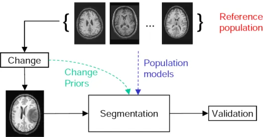
Figure 1.5. A conceptual overview of the proposed dissertation topic. It involves a segmentation framework which treats healthy adults as the refer-ence population and tumor as a change process, and a validation framework for the segmentation results. The segmentation framework makes use of reference population models and priors on the change processes. The vali-dation framework simulates the change processes to obtain known ground truth.

framework for brain MR images, extending applications to image data

pre-senting pathology or neurodevelopmental and neurodegenerative changes.

Considering the lack of a reliable ground truth, the reference population

model and deterministic models of the anatomical deviations can also be

combined to create synthetic ground truth. This facilitates objective

evalu-ation of the performance of different segmentevalu-ation methods.

(19)

Segmentation of MR images with pathological deviations, such as brain tumor, has been approached in different ways [13, 31, 47, 33]. The previously available tumor seg-mentation methods are not fully automatic and do not provide segseg-mentations of healthy tissue and edema. Detailed review of other segmentation approaches for brain tumor MRI is covered in Section 3.1. Review of other segmentation approaches for newborn brain MRI is presented in Section 4.1. The segmentation framework proposed in this dis-sertation is fully automatic and provides a complete description of the 3D brain anatomy. With regard to the simulation of MR images with pathological deviations, there is a lack of models that make use of relevant biological models. For example, the brain tumor MRI simulator proposed by Rexilius et al. [79] determines edema regions by using the white matter mask and distances to tumor boundary, and restricts contrast enhancement to the brain tumor regions. The brain tumor MRI simulation framework proposed in this dissertation uses a model of local diffusion properties for edema and computes contrast enhancement in both tumor and blood vessel regions.

My work as presented in this dissertation expands the previous work done by others in the field of Bayesian image segmentation and simulation of brain pathologies. The contributions of this dissertation are as follows:

(1) Image segmentation using a modified Expectation-Maximization (EM) algo-rithm: the novelties of this approach are its use of robust parameter estima-tion techniques and its automatic detecestima-tion of the feature space clusters for the mixture model.

(2) Generation of an augmented feature space for image segmentation through the use of spatial constraints such as location, curvature, and adjacency.

(3) Application of the proposed segmentation framework for healthy brains as well as images that exhibit deviations due to pathology (brain tumor) and growth (newborn brains).

(20)

(4) A method for generating pathological ground truth (tumor and edema) from im-age data with known healthy ground truth by combining a linear elastic biome-chanical model with random surface tractions and a reaction-diffusion process guided by diffusion tensor imaging (DTI). The simulation of a new pathological ground truth is guided by the underlying biological processes.

(5) Simulation of the accumulation of contrast agent for a brain tumor subject to generate contrast enhanced T1w MRI, which is the standard diagnostic imag-ing modality. The accumulation model is guided by the underlyimag-ing biological processes.

(6) Simulation of MR images with brain tumor and edema using textures synthe-sized from real tumor MRI samples. The synthetic MR images and the associated ground truth provides the means for objective evaluation of different segmenta-tion schemes.

1.4. Overview of Chapters

The remainder of this dissertation is organized as follows:

Chapter 2 presents the background material for Bayesian image segmentation with the maximum likelihood approach. This chapter also proposes a modification of the standard EM algorithm for computing the maximum likelihood estimate using robust parameter estimation techniques to detect deviations or noise.

Chapter 3 presents the application of the robust maximum likelihood image segmen-tation framework described in Chapter 2 for segmenting MRI of adult brains with tumor. The anatomical deviations from the adult brain atlas involve the deformation of healthy tissue due to tumor mass effect and the infiltration of the regions surrounding tumor by edema.

(21)

early growth pattern is treated as an anatomical deviation compared to the child brain atlas, where white matter appears as two distinct regions.

Chapter 5 describes the challenges and goals of validating segmentation results where the ground truth is difficult to obtain. In this chapter, I will develop a framework for generating synthetic brain tumor MR images with the associated ground truth based on the simulation of tumor and edema growth processes.

Chapter 6 concludes with a summary of the contributions and discussion of possible future work.

(22)

CHAPTER 2

Maximum Likelihood Image Segmentation

This chapter describes the image segmentation framework that forms the main con-tribution of this dissertation. Section 2.1 discusses the basic concepts for Bayesian image segmentation. Section 2.2 describes the segmentation process by maximizing the image likelihood using the Expectation-Maximization (EM) algorithm. Methods for estimating model parameters from noisy data with outliers are discussed in Section 2.3. Finally, extensions to the EM algorithm for segmenting images with deviations from an expected model is presented in Section 2.4.

2.1. Background

An image I = (Ik) is a collection of values arranged in a regular lattice Λ. In this

dissertation, Λ refers to the 3D image lattice, where the gaps in the lattice configuration can be different for each dimension. For every k ∈ Λ, Ik represents the feature values

associated with the voxel location k. In the case of multi-modal images, such as color images, Ik is a vector containing a fixed number of scalar component values. Image

segmentation is the task of assigning labels to each image location based on the feature values. This results in what is typically called the segmented image or the label image

S = (Sk). The valueSk is an assignment label drawn from a finite set of classes or labels

C or Sk∈ C.

(23)

provides a framework for estimating a map from an image I into a label imageS, while balancing the prior knowledge information and the observed data.

There are three essential probability distributions functions involved in the Bayesian framework. Thepriordistribution embodies the knowledge of likely configurations before an actual image is observed. In contrast, the probability distribution that is derived after an observation has been made is called theposteriordistribution. Thelikelihoodis defined as the probability of obtaining a particular observation given a set of model parameters (a conditional probability).

The theorem proposed by Bayes [7] describes the relation between the posterior prob-ability p(B|A), prior probability P r(B), and likelihood p(A|B).

Theorem 2.1. Bayes’ theorem states that the posterior probability p(B|A) is

propor-tional to the likelihood p(A|B) multiplied by the prior P r(B).

p(B|A) = p(A|B)P r(B)

p(A) (2.1.1)

Within a Bayesian framework, segmentation of a given image is performed by estimat-ing the label assignments and the parameters describestimat-ing the image appearance and/or geometry. The label image S and the model parameters θ form a tuple that describes the world state that generates the image I,

W = (S, θ).

Bayes estimators that map the imageI into the segmentationScan be constructed using the joint probability p(I, W). When the joint probability function is known, a simple estimator is to choose the most likely estimate ˆW that maximizes p(I, W). In practice however, the full joint probability is typically very complex thus most estimators use the associated conditional probabilities instead.

(24)

2.2. Image Segmentation using Expectation-Maximization

One can consider segmentation as a problem of finding the hidden label assignments from the observed image data. The Maximum Likelihood (ML) segmentation estimate is the one that maximizes the likelihood of observing the complete data J = (I, S) given the model parameters θ: p(J|θ), which is an associated conditional probability of p(I, W). When the parameters θ are known the estimate of the segmentation S is straightforward. On the other hand, when the hidden segmentation S is known we can infer the model parameters θ. This leads to the development of the well known Expectation-Maximization (EM) algorithm [25] for ML estimation.

The Expectation-Maximization algorithm can be considered as an optimization tech-nique where we maximize the lower bound for the image likelihood function [67]. The lower bound is derived from Jensen’s inequality:

X

j

g(j)aj ≥

Y

j

g(j)aj _(2.2.1)

given P

jaj = 1. In image segmentation, the EM algorithm finds the parameter which

maximizes the probability of a configuration over all the possible values for the hidden label assignment. The function that is maximized is:

f(θ) = p(I|θ) = X

S

p(I, S|θ). (2.2.2)

We can create a lower bound forf(θ) by using a probability function q(S) and applying Jensen’s inequality (Equation 2.2.1)

f(θ) =X

S

p(I, S|θ)

q(S) q(S) ≥ g(θ, q) =

Y

S

p(I, S|θ)

q(S)

. (2.2.3)

(25)

yields

log g(θ, q) = X

S

log

p(I, S|θ)

q(S)

= X

S

q(S)logp(I, S|θ) q(S)

= X

S

q(S)log p(I, S|θ)−q(S)log q(S). (2.2.4)

The probability ratio within the log term can be rewritten as follows:

p(I, S|θ)

q(S) =

p(S|I, θ)

p(I, S|θ)

q(S) =

p(S|I, θ)

q(S)

p(I, θ)

p(θ) =

p(S|I, θ)

q(S) p(I|θ).

Thus, obtaining the following interpretation for the log of the bound that defines the optimalq(S) [11]:

log g(θ, q) = X

S

q(S)logp(I, S|θ) q(S)

= Eq(S){log

p(S|I, θ)

q(S) }+log p(I|θ)

= −Eq(S){log

q(S)

p(S|I, θ)}+log p(I|θ)

= −DKL(q(S)||p(S|I, θ)) +log p(I|θ) (2.2.5)

where E is the expectation function and DKL is the (non-negative) relative entropy or

Kullback-Leibler divergence [49]. To obtain the optimal q(S) for the bound, we need to minimize the relative entropy between q(S) and the label posterior probability. This can be achieved when this divergence is made zero by using the same probability function,

q(S) = p(S|I, θ). Computing q to obtain a good bound on the expected likelihood is called the E-step, while maximizing the bound over θ is called the M-step. With regard to image segmentation, the estimation of the hidden segmentation labels is called the E-step and the estimation of the best parameters θ from the complete labeled image data is called the M-step.

(26)

The Kullback-Leibler divergence has also been demonstrated to be a useful metric for defining average anatomies, as proposed by Lorenzen et al. [56, 55]. In this case, the divergence is minimized in order to maximize a lower bound on the Bayes probability of error between the average anatomy and the set of subject anatomies. This is similar to the maximization of a lower bound on complete data likelihood in the EM algorithm. Maximizing the Bayes probability of error ensure that the average anatomy resembles the actual observed anatomies.

The EM algorithm computes the ML estimate through an iterative process. In one iteration it performs the estimation of theq(S) function given the current model param-eters and the calculation of the model paramparam-eters θ that maximizes the complete data likelihood p(J|θ). During the nth iteration the algorithm proceeds as follows:

• E-step: Given the observationI and the current model parameterθ(n), compute the conditional expectation of the complete data likelihood defined asQ(θ|θ(n)_),

Q(θ|θ(n)) =E_p₍_S|I,θ(n)₎{log p(J|θ)}=E_p₍_S_|_I,θ(n)₎{log p(I, S|θ)}. (2.2.6)

The goodness-of-fit function Q is derived by extracting the relevant term from Equation 2.2.4 and substituting q(S) with the optimal probability function

p(S|I, θ).

• M-step: Update the model parameters for the next iteration so that the expected

complete data likelihood is maximized,

θ(n+1) = arg max

θ

Q(θ|θ(n)). (2.2.7)

(27)

guarantees that the log-likelihood log p(J|θ) is increased [103]. The GEM algorithm in practice converges to a local maxima given a particular initialization, which makes it particularly sensitive with regard to its initial values.

Here, I will develop an EM image segmentation algorithm using a Gaussian mixture model for multi-modal images with voxel data in _Rd_{. This is a standard approach that}

has been used for medical image segmentation by Wellset al. [100], van Leemputet al.

[93], and Zhanget al. [106]. Image segmentation using EM is an iterative process where we begin with a model parameters θ(0)_{. Each segmentation iteration involves estimating} the segmentation labels and updating the model parameters. The complete image data at different locations are assumed to be statistically independent, Ju ⊥⊥ Jv∀u 6= v. For

each location k, the appearance model or the individual image likelihood for a specific label or class cis

p(Ik|Sk=c, θ) = Nµc,Σc(Ik) (2.2.8)

where Nµc,Σc is the multivariate normal distribution associated with class c with mean

µc and covariance matrix Σc. The model parametersθ are composed of parameter values

for the class-specific multivariate normals, θ = {(µi,Σi)∀i ∈ C}. With the voxelwise

independence assumption the image likelihood becomes

p(I|W) =p(I|S, θ) = Y

k

p(Ik|Sk, θ). (2.2.9)

In the case of natural images, the prior probabilities at specific locations P r(Sk) are not

known. A common approach is to choose a global value ρc for a class label c based on

experiments or prior knowledge, P r(Sk =c) = ρc∀k. In the case of anatomical images,

the prior probabilities for specific structures are known to some degree. For example, the likely spatial configuration for the brain can be described reliably using the spatial priors

P r(Sk=c) which describes the probability of observing an anatomical component of the

brain (labeled by c) at location k. In Chapters 3 and 4, the spatial priors from the brain atlas will be used to segment real brain MRI. The use of an explicit, predefined spatial priors is relevant for medical images since we have known structures or anatomy.

(28)

The probabilistic models of p(Ik|Sk = c, θ) and P r(Sk) are the main components

for ML estimation. Combining the image likelihood function (Equation 2.2.8) with the voxelwise-independence assumption leads to the following complete data likelihood func-tion:

Q(θ|θ(n)) = X

c

X

k

log[p(Ik, Sk=c|θ)]p(Sk =c|Ik, θ(n))

= X

k

X

c

log[p(Ik|Sk=c, θ)P r(Sk=c)]p(Sk=c|Ik, θ(n))

= X

k

X

c

log[Nµc,Σc(Ik)P r(Sk =c)]p(Sk =c|Ik, θ

(n)₎_. _(2.2.10)

The best estimate for the model parameters θ can be found through explicit maximiza-tion, i.e. determining the µc and Σc values that satisfy the conditions ∂Q(θ

|θ(n)₎

∂µc = 0 and

∂Q(θ|θ(n)₎

∂Σc = 0. This leads to the following update equations for the M-step:

w_k,c(n+1) = p(Ik|Sk=c, θ

(n)₎_{P r}₍_S

k)

P

c0p(Ik|Sk=c0, θ(n))P r(Sk)

(2.2.11)

µ(_cn+1) =

P

kw

(n+1)

k,c Ik

P

kw

(n+1)

k,c

(2.2.12)

Σ(_cn+1) =

P

kw

(n+1)

k,c (Ik−µ

(n+1)

c )t(Ik−µ

(n+1)

c )

P

kw

(n+1)

k,c

(2.2.13)

Equation 2.2.11 describes the weight values for the expected likelihood in the E-step,

w(_k,cn) = p(Sk = c|I, θ(n)). The update equations for the image model with

voxelwise-independent normal distributions show that model parameters for the next iteration are the the mean and covariance values of the image intensities, weighted by the normalized class posterior probabilities. In this example, image segmentation can be reduced to the following iterative steps:

(1) Estimating the initial model parameters θ(0). This can be achieved through unsupervised clustering [100, 106] or using a spatial prior such as the brain atlas [93, 17].

(29)

(3) Updating the mean and covariance parameter values using the observed image intensity values.

(4) Repeat the second and third step until convergence to a local maxima.

(5) Obtaining final segmentation labels from the class posterior probability. For discrete labels, the classification label Lk for locationk is obtained as follows:

Lk = arg max c

p(Sk =c|Ik, θ(nf inal)). (2.2.14)

The ML image segmentation framework does not yield a true Bayes estimator for the world state W. Although the ML framework makes use of the class prior probabilities

P r(Sk), it does not include the modeling of P r(W) =P r(S, θ) or even P r(θ). For the

example framework described above, this is not a major issue since the model parameters

θ are simply the means and covariances for the image likelihood described using normal distributions. However, when the model parameters θ become more sophisticated the use of prior knowledge of θ can improve the segmentation performance. Appendix B discusses a framework using a true Bayes estimator, where one can make use of the prior

P r(W).

2.3. Robust Parameter Estimation

Estimating the model parameters θ in the M-step is a critical part of the EM algo-rithm. The original EM formulation computes the means and covariances of the Gaussian mixture model without taking account of possible outliers in the image data. I propose to improve the EM algorithm by using robust parameter estimation in the M-step in place of the standard approach. There has been some limited previous work for this type of ap-proach, where robust estimation is combined with the EM algorithm. Malyutov and Lu [59] used the robust least median of squares and the M-estimator for estimating object trajectories from frame sequences that are corrupted with noise and clutter (correlated noise). With regard to medical image segmentation, van Leemput et al. applied the M-estimator for detecting brain lesions from MRI [95]. Their approach uses a multiplier

(30)

for the E-step weights, effectively deweighting based on intensity thresholding through the following equation:

q0(Sk) =

p

p+I{Ik > threshold}κ

q(Sk) (2.3.1)

where p is the Gaussian likelihood for healthy brain tissue, I is the indicator function, and κ is the class-specific deweighting parameter based on the covariance determinant. The intensity thresholding is done relative to the class intensity means. The means are computed as the weighted averages of the relevant image data values, which may be skewed by outliers. Equation 2.3.1 assigns lower probablity of healthy tissue in regions that fit the criteria of being abnormal (in this case lesions).

Estimators using weight functions such as the M-estimator typically cannot handle large proportion of outliers in data since they have a low breakdown point [12]. The breakdown point is defined as the fraction of data that must be moved to infinity (i.e., become outliers) for the method to generate inaccurate results. In fact, the classic un-bounded M-estimators has a breakdown point of 0 [86] since a single outlier with feature values that are significantly different from most of the data can lead to a local minima. In practice, the M-estimator typically have an approximate breakdown point of 0.15 to 0.2. The method proposed by van Leemput et al., while performing well on brain lesion data, can fail when used to segment images with significant proportion of outliers due to malignant pathology or growth changes. In this dissertation, I propose the use of meth-ods with a high breakdown point such as a combinatorial robust parameter estimator (Section 2.3.1) and a graph-based parameter estimator (Section 2.3.2). These methods isolate the clusters within data while taking account of outliers. They can be used in place of the standard M-step to generate parameters that are not unduely influenced by data outliers.

(31)

the lowest determinant of covariance. The generated estimate is highly robust with a high breakdown point. The MCD estimator has a breakdown point of 0.5, more than half of the data needs to be contaminated to make the results be unreasonable.

Rousseeuw and van Driesen [80] proposed a fast algorithm that computes an approx-imation of the MCD estimate. The algorithm first creates several initial subsets, where the elements are chosen randomly. From each subset, the algorithm determines different initial estimates of the robust mean and covariance. The estimates are then refined by performing a number of C-step operations on each initial selections. A single C-step operation consists of the following steps:

(1) Given a subset of the data, compute the mean and covariance of the elements in the subset.

(2) Compute Mahalanobis distances of the data elements in the whole set. (3) Sort points based on distances, smallest to largest.

(4) Select a new subset where the distances are minimized (i.e. the first half of the whole set of the sorted data points).

An illustration of a single C-step iteration is shown in Figure 2.1. A C-step operation will result in a subset selection that yields a determinant of covariance less or equal to the one obtained from the previous subset. The iterative applications of C-steps yield final estimates with the smallest determinant of covariance. From all the final estimates computed with different initial selections, the mean and covariance estimate with the smallest determinant of covariance is chosen as the robust estimate.

2.3.2. Minimum Spanning Tree Clustering. The Minimum Spanning Tree (MST) clustering algorithm is a graph based techniques that yields a predefined number of data clusters while ignoring outliers. Unlike the MCD estimator that only provides a single data cluster, MST clustering can yield two or more data clusters.

Given a graphG= (V, E) with verticesV and edgesE, the Minimum Spanning Tree [21] is a graph GM ST = (V0, E0) where all the vertices are connected such that the total

(32)

Figure 2.1. An illustration of a single C-step iteration, a key component of the MCD robust estimation algorithm. Left: original 2-D data withM

points. Center: random selection of a subset of the data (marked with circles). Right: the selection after a C-step iteration, where the first M/2 closest points to the previous mean and covariance estimates are selected. The ellipsoidal curves in the center and right plots show the locations one standard deviation away from the mean and covariance estimates, which are computed from the selected points.

edge lengths are minimized. The MST graph is a subset of the original graph G, V0 ⊆V

and E0 ⊆E, where E0 does not contain any closed loops (cycles).

The MST-based clustering technique proceeds by first creating the MST graph from the sampled data (image intensities) and then iteratively breaking the long edges to form connected clusters. At each iteration, it breaks an undirected edgee(v, w) that connects vertices v and w if its length is larger than A(v)×T or A(w)×T. A(v) is the average length of edges incident on vertex v. Given N(v) as the set of neighboring vertices for a vertex v, A(v) = _|_N1₍_v₎_|P

q|e(v, q)|, where q ∈ N(v). T is a scalar distance multiplier

that determines which edges are considered to have significant deviation from the edges in the neighborhood.

(33)

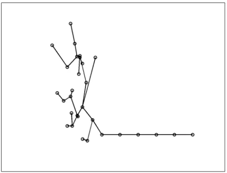
Figure 2.2. Clustering by breaking the long edges of a Minimum Span-ning Tree. Left: the MST created from the input data, with the long edges broken. Right: the generated clusters, note that the isolated far away points are treated as outliers and are not included.

at least two large data clusters where one of them is very dark and another is relatively bright.

The MST clustering algorithm uses the local propertyA(v) for a vertexvto determine the clusters, as opposed to the combinatorial MCD scheme which involves large subsets of data. This can cause problems when the global configuration of the data in feature space is not optimal. The breakdown point can be as low as zero when the actual data samples and the outlier samples are connected by a series of short, equal-length edges. Figure 2.3 shows an example of a configuration that leads to a low breakdown point. This configuration will cause the algorithm to fail in detecting the separation between data and outliers. However, this type of configuration is not generic and rarely occurs with real data. Some heuristics can also be applied to avoid having a sequence of short edges, such as the one presented in Chapter 4. Assuming typical sample configurations for the input and picking the largest data cluster as inliers, the MST clustering algorithm can have a breakdown point as high as 0.5.

Details on the properties of the MST graph structure can be found in the book by Cormen et al. [21]. Applications of graph-based clustering for pattern recogniction is described in the book by Dudaet al. [27]. Of relevance to this dissertation, a description

(34)

Figure 2.3. An example configuration where the Minimum Spanning Tree clustering cannot properly separate outliers from data. The outlier points on the lower right are connected by relatively short and equal-length edges. These edges will only be broken when some of the edges connecting the inlier samples are also broken, which leads to a skewed estimate of the inlier distribution.

of the robust MST clustering method applied to the segmentation of medical images can be found in the paper by Cocoscoet al. [17].

2.4. Robust EM Segmentation Framework

(35)

I propose the modification of the EM algorithm into a new robust EM algorithm, where the parameter update in the M-step is replaced with a robust parameter estima-tor described in the previous section. This makes it suitable for detecting anatomical deviations in medical images, as they can alter significant proportions of the image data. Since real images can have specific and complex appearance properties, the Gaussian mix-ture model in the EM image segmentation may not always be appropriate. To improve segmentation results in the general case, I propose the use of non-parametric density functions for the image likelihood. Instead of computing the Gaussian distributions for

p(I|W), the algorithm computes non-parametric kernel density estimates.

In the M-step, the robust data driven parameter estimation methods (the Minimum Covariance Determinant estimator and the Minimum Spanning Tree clustering) are used to generate data clusters together with the knowledge of data outliers. The knowledge of the relevant clusters allows the method to robustly determine the proper intensity ranges for the major structures. The generative model p(I|W) is estimated by fitting a probability distribution to the data clusters, performed by using the data within each cluster as training data for the nonparametric kernel densities.

The new robust EM algorithm is an iterative process that replaces the parameter update equations (Equations 2.2.12 and 2.2.13) with the combination of robust data clustering and non-parametric density estimation. The modified algorithm proceeds as follows in thenth _iteration:

• E-step: This part of the EM algorithm is unchanged. The goodness-of-fit function Q is computed according to Equation 2.2.6 using the class posteriors

p(S|I, θ(n)_{) to form the expectation.}

• M-step: Computation the updated parametersθ(n+1) is done through clustering of image data samples. The samples are obtained using the parameters from the current iterationn, which determines the class posteriorsp(S|I, θ(n)_{). The class} posteriors describe the likely regions for obtaining data samples. Good regions

(36)

for sample selection are determined by thresholding the current class posteriors or using a Monte Carlo approach (e.g., the Metropolis-Hastings algorithm).

Once the clusters are identified, the individual mixture components p(I|S=

c, θ) are computed by fitting a kernel density function to the intensity data within the clusters. The samples form the training data for classification using non-parametric density mixtures. For a classcand voxel location k the updated voxel image likelihood becomes

p(Ik|Sk =c, θ(n+1)) =

1

M

X

i=1

Kλ(Ik−Y

(n)

i ) (2.4.1)

whereKλ is the multivariate Gaussian kernel with standard deviationλand zero

mean, and Y(n) is the set of M training samples obtained by applying robust clustering to samples fromp(S|I, θ(n)_{). The choice of the standard deviation or} kernel width λ is crucial in determining the classification decision boundaries. The kernel width can be estimated through heuristics, for example by choosing a fraction of the expected image intensity range. The kernel width can also be estimated using a bootstrap technique.

Initialization of the robust EM algorithm is performed by using the spatial priors provided by the atlas, p(Sk = c|Ik, θ(0)) = P r(Sk = c). Each iteration of the robust algorithm

refines the class posterior probability p(Sk = c|Ik, θ(n)) and tends to result in sharper

spatial posterior probabilities.

(37)

image gradient magnitude values (Section 4.2). This approach samples smooth image regions, which results in coherent data clusters that are easier to detect and to separate. Using knowledge on the geometric configuration within the images avoid contaminating the samples with ambiguous data or data which induces a certain bias in parameter estimation.

The classic EM algorithm with mixture models restricts the number of mixture com-ponents to a predetermined value. This model is inappropriate for many real images, as objects may enter and leave the scene or pathological structures can be formed or can disappear, for example. I propose a modification of the classic EM algorithm where new mixture components are detected through explicit detection of multiple clusters within the data. The detection of multiple clusters can be achieved in a robust manner that discards outliers by using the robust MST clustering proposed in the previous section. The existence of new mixture components can be tested by evaluating the amount of overlap between the detected clusters from the MST graph. This detection of new mix-ture components is applied to the determination of possible edema surrounding tumor in Section 3.2.

The robust image segmentation framework includes modifications that make it no longer a true EM algorithm. The log likelihood Q is no longer guaranteed to increase at every iteration. Therefore, the iterative process is terminated when the change is smaller than a threshold:

|Q(θ

(n+1)_|_θn₎₋_Q₍_θn_|_θ(n−1)₎

Q(θn_|_θ(n−1)₎ | < Q (2.4.2) The robust EM image segmentation framework performs classification mainly based on the image intensity feature space data. If available, the spatial information from the brain atlas prior P r(S) is combined with the class likelihood using the Bayes rule. The spatial priors P r(S) may be suboptimal since there may exist some deviations between the data and the prior model. In cases with small to moderate deviations, classification using the intensity feature space can still be reliable due to the use of the robust parameter estimation techniques. However, in cases with large deviations, the use of the spatial prior

(38)

P r(S) may result in samples that have a significant proportion of outliers. When the proportion of outliers exceed the breakdown point of the robust parameter estimator, the algorithm would fail to estimate the proper image likelihood and the segmentation would fail. To deal with this issue, it will be necessary to explicitly account for possible changes toP r(S) to form an appropriate model for the observed images. As an example, spatial priors coded in the healthy adult atlas need to account for brain tumors that can deform surrounding structures.

Another limitation of the algorithm is related to the voxel-based approach, where it is assumed that each voxel is independent to other voxels. This approach can lead to spurious segmentations where small collections of voxels within some regions are incor-rectly labeled as distinct from the surrounding labels. Noisy results can be avoided by extending the framework via the application of a Markov Random Field (MRF) model to P r(Sk), similar to the approach proposed by van Leemput et al. [93] and Zhang et al. [106]. However, the MRF model tends to smoothen the segmented structures and thus may not be appropriate for some applications where we require segmentations with fine details. An alternative to the MRF approach would be the use of an extended image model with a modeling of image region coherence and the more complete prior P r(S, θ) rather than onlyP r(S). Such an extended model is proposed in a Maximum a Posteriori (MAP) image segmentation framework discussed in Appendix B.

(39)

CHAPTER 3

Brain Tumor MRI Segmentation

In this chapter, I will describe the application of the robust EM framework described in Chapter 2 to automatic brain tumor segmentation from MRI. Section 3.1 provides a discussion of the motivation and challenges in segmenting brain tumor MR images. The adaption of the robust EM image segmentation framework to accomodate pathol-ogy is described in Section 3.2. Deviations in intensity and appearance due to tumor and edema are detected as outliers from the expected image model of healthy tissue. Existence of edema is determined automatically by testing for a bimodal distribution of the outlier samples. In Section 3.3, I present the results of the automatic segmentation framework applied to three different types of tumor, along with the validation of those results compared to manual segmentations.

3.1. Background

(40)

For many human experts, manual segmentation of brain tumor from MRI is a difficult and time consuming task. Therefore, an automated brain tumor segmentation method is desirable. There are many potential applications of automated segmentation. The changes of healthy tissue due to tumor and edema need to be identified for determining surgical and radiological treatment planning. The knowledge of affected regions is also vital for studying possible diagnostic markers for brain tumors. For example, the shape of blood vessels within tumor regions is observed to have significant correlation with tumor classification into benign and malignant types [10].

The multiple challenges associated with automatic brain tumor segmentation have given rise to many different approaches. Automated segmentation methods that combine fuzzy clustering and knowledge-based classification were proposed in [13, 31]. The two methods do not rely on intensity enhancements provided by the use of contrast agents. A particular limitation of the two methods is the use of specific classification rules which restricts the image modalities to the T1, T2, and PD weighted MR image channels. Additionally, the methods require a manually guided training phase prior to segmenting a set of images. Other methods are based on statistical pattern recognition techniques, for example the method proposed by Kaus et al. [48]. This method combines the information from a registered atlas template and user input to supervise training of a the classifier, demonstrating the strength of combining voxel-intensity with geometric brain atlas information. This method was validated against meningiomas and low-grade gliomas. Geringet al. [33] proposed a method that detects deviations from normal brains using a multi-layer Markov random field framework. The information layers include voxel intensities, structural coherence, spatial locations, and user input. Cuadra et al.

presented high-dimensional warping to study deformation of brain tissue due to tumor growth [22]. Their technique relies on a prior definition of the tumor boundary whereas the method proposed in this chapter focuses on automatically finding tumor regions.

(41)

blobby shaped tumors with uniform intensity. Even though the intensity enhancement can aid the segmentation process, it is not always necessary to obtain good results. In fact, requiring the use of contrast enhancement to segment tumors can be problematic. Typically, tumors are only partially enhanced and some tumors are not enhanced at all. Blood vessels also generally appear enhanced by the contrast agent. These inconsis-tencies create an ambiguity in the image interpretation, which makes the T1-enhanced image channel a less than ideal feature for tumor segmentation in general. Methods that primarily use the contrast enhancement to drive the tumor segmentation will have difficulties in isolating tumors.

Edema surrounding tumors and infiltrating mostly white matter was most often not considered as important for tumor segmentation. It has been shown previously [71, 77] that edema can be segmented using a prior for edema intensity and restriction to the white matter region. The extraction of the edema region is essential for diagnosis, therapy planning, and surgery. It is also essential for efforts that involve modeling the brain deformation due to tumor growth. The swelling produced by infiltrating edema usually has distinctly different tissue property characteristics than space occupying tumor. The segmentation strategy presented in this chapter is based on the detection of changes from normal and will thus systematically include segmentation of edema. Differential identification of the two abnormal regions tumor and edema is clinically highly relevant. Even though the primary therapeutic focus will be on the tumor region, the edema region may require secondary analysis and treatment.

The proposed method combines a model of normal tissues and the geometric and spatial model of tumor and edema. It relies on the information provided in the T2 weighted image channel for identifying edema, and it can make use of additional image channels to aid the segmentation. Here, I have chosen to use only the T1 and T2 image channels. Tumor and edema are treated as intensity abnormalities or outliers. After identifying the abnormalities, an unsupervised clustering technique is applied to the intensity features before utilizing geometric and spatial constraints. I will show that this

(42)

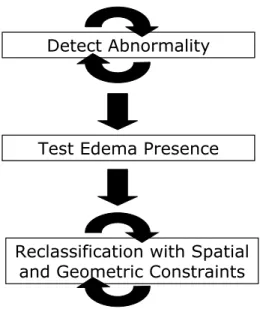
Detect Abnormality

Test Edema Presence

Reclassification with Spatial and Geometric Constraints

Figure 3.1. The three major stages of the brain tumor MRI segmentation method.

method can segment tumors with or without intensity enhancements and automatically detects the presence of edema. This approach offers a means of approaching lesions of multiple types and of different image intensities, and, with a single method, lesions that enhance or do not, and that may or may not be surrounded by edema.

3.2. Method

The automated segmentation method for brain tumor MRI is composed of three major stages, as shown in Figure 3.1. First, it detects abnormal regions, where the intensity characteristics deviate from the expectation. In the second stage, it determines whether these regions are composed of both tumor and edema. Finally, once the estimates for tumor and edema intensity parameters are obtained, the spatial and geometric properties are used for determining proper sample locations. The details of each stage are discussed in the following subsections.

(43)

Figure 3.2. The brain atlas that acts as the model of the healthy adult population, provided by the International Consortium for Brain Mapping (ICBM). From left to right: the T1 template image and probability values of white matter, gray matter, and cerebrospinal fluid. The atlas does not account for brain tumor and edema, thus its use for segmentation of images presenting pathology requires a new approach.

obtained by sampling specific regions based on the probabilistic brain atlas for healthy adults shown in Figure 3.2 [28].

The atlas is aligned with the subject image data by registering the atlas template image with the subject image. The registration is performed using affine transformation with the mutual information image match measure [58]. After alignment, the samples for each healthy class (white matter, gray matter, and cerebrospinal fluid) are obtained by randomly selecting the voxels with high atlas probability values. The set of training samples is constrained to be the voxels with probabilities higher than a thresholdτ = 0.85 [17].

The training data for the healthy classes generally contain unwanted samples due to contamination with samples from other tissue types, particularly tumor and edema. The pathological regions are not accounted for in the brain atlas and they therefore occupy regions that are marked as healthy. The contaminants are considered data outliers, and they need to be removed so that the training samples for the healthy classes are representative. The samples are known to be contaminated if their characteristics differ from prior knowledge. The intensities for healthy classes are known to be well clustered and can be well approximated using Gaussians (Figure 3.3).

Handling data outliers is a crucial step for atlas based image segmentation. Cocosco

et al. [17] developed a segmentation method for healthy brains that builds the Minimum Spanning Tree from the training samples and iteratively breaks the edges to remove false

(44)

Figure 3.3. Example healthy adult MRI dataset. Top, from left to right: T1 image, T2 image, and segmentation labels (red is white matter, green is gray matter, and blue is cerebrospinal fluid). Bottom: the intensity histogram for the three classes, the horizontal axis represents T1 intensities and the vertical axis represents T2 intensities. The intensity features for each class is tightly clustered and can be approximated with a Gaussian.

positives (pruning). They showed that pruning the training samples results in significant improvement of the segmentation quality, particularly for image data presenting enlarged ventricles. In my method, robust estimate of the mean and covariance of the training data is used to determine the outliers to be removed.

(45)

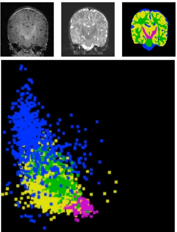
Figure 3.4. The white matter training data for a subject with tumor and edema, the horizontal axis represents the T1 intensities and the ver-tical axis represents the T2 intensities. Left: original samples obtained by atlas-guided sampling which is contaminated with samples from other distributions. Right: remaining samples after trimming using the robust MCD estimate, representing the feature distribution of healthy white mat-ter.

shown in Figure 3.4 for white matter samples. The inliers of the healthy brain tissue class samples are used as training samples for estimating the corresponding density functions. The specific aim at this stage is to compute the density estimates and posterior probabilities for the set of class labels C = {white matter, gray matter, csf, abnormal, non-brain}. A parametric density function is not ideal for the case of tumor segmentation. Tumors do not always appear with uniform intensities, particularly in the case where some tissues inside the tumor are necrotic tissues. Therefore, no assumption can be made regarding the intensity distributions and thus I use a non-parametric model for the probability density functions. The density functions are approximated using kernel expansion or Parzen windowing [27]. Given the vector of intensity featuresIkat location

k, the probability density function on intensity for class labelSk =cis

p(Ik|Sk =c, θ= (λ, Y)) =

1

N

X

i=1

Kλ(Ik−Yi) (3.2.1)

where Kλ is the multivariate Gaussian kernel with standard deviation λ, and Y is the

set of class training samples. The kernel bandwidthλ chosen is 4% of the intensity range for each channel, determined using empirical tests on multiple images.

(46)

The posterior probability at location k is computed using the class prior probability from the atlas P r(Sk) by applying the Bayes rule

p(Sk|Ik, θ) =

p(Ik|Sk, θ)P r(Sk)

p(Ik)

. (3.2.2)

The spatial priors for white matter, gray matter, csf, and non-brain classes are the corresponding atlas probabilities. For the abnormal class, a fraction of the sum of white matter and gray matter atlas probabilities is used since tumor and edema usually appear in these regions and not in the csf regions. With the kernel density estimate as the likelihood, the image appearance parameters θ for tumor segmentation is composed of the set of training samples for each class and the kernel width.

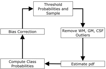
An issue with MR images is the presence of the image inhomogeneity or the bias field. This is dealt by interleaving the segmentation process with bias correction, following the spirit of [100]. The entire process of detecting the abnormal regions is shown in Figure 3.5, a loop that is composed of the following five stages:

(1) Threshold the class posterior probabilities and sample the high confidence re-gions. The posterior probabilities are initialized using the prior probabilities obtained from the brain atlas.

(2) Remove the samples for normal tissues that exceed a distance threshold based on the MCD estimate.

(3) Estimate the non-parametric density for each class likelihood using kernel ex-pansions. The initial density for the abnormal class is set to be uniform, which makes this class act as a rejection class. The brain voxels with intensity features that are different from those of healthy classes or not located in the expected spatial coordinates will be assigned to this class.

(4) Update the class posterior probabilities using the new class likelihoods.

(47)

Threshold Probabilities and

Sample

Bias Correction Remove WM, GM, CSF

Outliers

Estimate pdf Compute Class

Probabilities

Figure 3.5. The process of detecting abnormal regions, the first stage of the brain tumor MRI segmentation method.

Initialization Iteration 1 Iteration 2 Iteration 3

Figure 3.6. Snapshots of the estimated probability density function of the abnormal class for the Tumor020 data. Each image shows the result of different iterations of the loop shown in the previous figure. The density is initialized so that all intensities are equally likely. The horizontal axis represents the T1 intensities and the vertical axis represents the T2 inten-sities. The two high density regions visible at the final iteration are the tumor and edema densities, which have a significant separation along the dimension of the T2 intensities.

The first major segmentation stage detects the abnormal regions by executing the loop for several iterations, obtaining the intensity descriptions for each class. The abnormal class density at different iterations for the Tumor020 data is shown in Figure 3.6.

The bias correction method is based on the one developed by van Leemput et al.

[92]. The method uses the posterior probabilities to estimate the homogeneous image. It then computes the bias field estimate, as the log-difference between the homogeneous images and the real subject images. The bias field is modeled as a polynomial, and the

(48)

coefficients of the polynomial is determined through least squares fitting. The method assumes that the class intensity distributions are approximately Gaussians. Only the white matter and gray matter probabilities are used for estimating the parameters for the bias field correction, as they generally can be approximated by Gaussians without significant errors. Additionally, the combination of white and gray matter probabilities represents a large connected region covering the major part of the brain.

3.2.2. Tumor and Edema Separation. The densities and posterior probabilities com-puted for the abnormal class in the previous stage give us a rough estimate of how likely it is that some voxels are part of tumor or edema. I make the assumption that the detected abnormal voxels are composed mostly of tumor and possibly edema. Edema is not always present when tumor is present, therefore it is necessary to specifically test the presence of edema. This is done by first obtaining the intensity samples for the abnormal region, which is performed by thresholding the posterior probabilities and selecting a subset of the high probability regions. The samples are then clustered and a test is done to determine whether there exist separate clusters for tumor and edema. The density estimate for tumor (and edema, if present) is obtained by performing kernel expansion on the samples.

Tumor and edema are generally separable given the information in the T2 weighted image (Figures 3.6 and 3.7). Edema has high fluid content and therefore appears brighter than tumor in this image channel. To separate the densities, unsupervised clustering is applied to the samples obtained by thresholding. The method I have chosen is k-means clustering withk = 2 [27]. For dealing with outliers, the robust MST clustering described in Section 2.3 can also be used as an alternative. Once the clusters are obtained, the tumor cluster can be identified as the cluster with the lower T2 mean value, making use of prior domain knowledge.

(49)

Figure 3.7. The T1 image (left) and the T2 image (right) from the Tu-mor020 data. The tumor and edema on the right part of the brain can be clearly differentiated based on the T2 intensities. As observed in the T2 image, the tumor region (rightmost) is darker than the surrounding edema region, as edema is composed mostly of fluid.

the mean value µtumor, and n candidate edema samples i with the mean value µedema,

the overlap measure is:

1 2

1

m

Pm

i=1||τi−µtumor||+ 1

n

Pn

i=1||i−µedema|| ||µtumor−µedema||

(3.2.3)

The T2 channel contains most of the information needed for differentiating tumor and edema. Therefore, the overlap is measured only for the T2 data dimension of each cluster. If the amount of overlap is larger than a specified threshold, then the tumor density is set to be the density for the abnormal class and the edema density is set to zero.

3.2.3. Application of Spatial and Geometric Constraints. Once this stage is reached, tumor and edema are already segmented based on atlas priors and intensity characteristics. However, voxel-based processing does not consider geometric and spatial properties and this generally leads to noisy segmentation results. Since there is no model for the intensity distributions of tumor and edema, it is necessary to use geometric and spatial heuristics to prune the samples that are used for estimating the densities. The prior knowledge used in this stage is the fact that tumor is mostly blobby. For edema, the applied constraint is that each edema region needs to be connected to a nearby tumor region. Some edema voxels can be located far away from tumor regions, but they must be spatially connected to a tumor region.

(50)

Tumor structures generally appear as blobby lumps, and this shape constraint is enforced through region competition snakes [84, 88, 89, 108]. The tumor posterior probabilities are used as the input for the snake, which is represented as the zero level set of the implicit function φ. The level set evolution is governed by the following equation [40]:

∂φ

∂t =α(p(Sk =tumor|Ik, θ)−p(Sk =tumor|Ik, θ))|∇φ| +β∇ ·

∇φ

|∇φ|

|∇φ| (3.2.4)

The propagation term is represented by α. It is modulated by the difference of the posterior probabilities for the tumor class and the non-tumor class (p(Sk =tumor|Ik, θ)

and p(tumor|Ik, θ)), so that the direction of the propagation is determined by the sign

of the difference. The probability that a voxel is part of brain and not part of tumor is represented by p(tumor|Ik, θ), more explicitly:

p(tumor|Ik, θ) = p({white matter}|Ik, θ) +p({gray matter}|Ik, θ) +p({csf}|Ik, θ)

+ p({edema}|Ik, θ) (3.2.5)

The snake shrinks when the boundary encloses part of the regions not part of tumor and expands when the boundary is inside the tumor region. Smoothing on the snake contour is applied using mean curvature flow, and the strength of this smoothing is controlled by theβ term. The initial level set function is obtained by performing a signed distance transform on the segmented tumor objects.

(51)

share some voxels with a tumor region are considered valid. Edema samples from these regions are kept, while other edema samples are discarded.

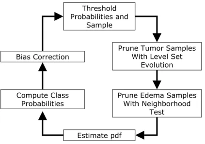
The final segmentation is obtained by reclassifying the image using the iterative steps similar to the one described in Section 3.2.1, with some modifications (Figure 3.8). The outlier removal stage is removed and there are additional steps where these geometric and spatial constraints are enforced. The entire loop is performed several times, after going through each loop the tumor and edema probabilities at the voxel locations that do not pass the tests are set to zero. This way, the segmentation for these locations are determined based on the next best candidate class. The tumor shape constraint is disabled at the last fitting stage. This is done to obtain the proper boundary for the tumor structures, which may not be entirely smooth. For instance, gliomas typically have a general blobby shape and ragged boundaries.

The application of geometric and spatial constraints modifies the M-step of the stan-dard EM algorithm so that it ignores the data samples obtained from inappropriate locations. This is a geometric-based approach to robust parameter estimation, where we make use of prior knowledge of the application domain with regard to spatial and geometric properties. This modification makes sure that the method can exclude subtle outliers (outliers located close to actual data clusters) by using the augmented features that include location and shape features.

(52)

Threshold Probabilities and

Sample

Bias Correction Prune Tumor Samples With Level Set

Evolution

Estimate pdf Compute Class

Probabilities Prune Edema Samples With Neighborhood

Test