DISEASE ASSOCIATED MUTATIONS AND FUNCTIONAL VARIANTS THAT SIGNIFICANTLY DISRUPT RNA STRUCTURE
Matt Halvorsen
A dissertation submitted to the faculty of the University of North Carolina at Chapel Hill in partial fulfillment of the requirements for the degree of Doctor of Philosophy in the Department of Bioinformatics and Computational Biology.
Chapel Hill 2013
Approved by:
Alain Laederach
Scott Hammond
Bill Marzluff
Karen Mohlke
Jan Prins
ABSTRACT
Matt Halvorsen: Disease associated mutations and functional variants that significantly disrupt RNA structure
(Under the direction of Alain Laederach)
Dedicated to. . .
My parents. For loving and supporting me, and for always believing in me even when I
myself did not.
Priya, my fiance. You have stuck with me through thick and thin, and I can’t begin to
ACKNOWLEDGEMENTS
I first want to say thank two large sets of people : the people from the Wadsworth Center in Albany, NY, where I started my PhD work, and the people here at UNC Chapel Hill, where I finished my work. The Wadsworth center is where a lot of the important work described in this paper was done, and while changing circumstances led to my having to leave alongside my lab to go to UNC, I won’t forget the people I met and worked with in Albany. I am grateful for my initial committee members Marlene Belfort, Joe Wade, Janice Pata, and Pan Li helping me along during the time when I was there. Additionally I wanted to acknowledge Andrew Reilly for providing our lab useful advice for our statistical analyses. Also I want to thank my fellow (at the time) grad students at Wadsworth, including Sneha, Kate, Stacey, Indrajit, Purba, and Brandon, for working together with me to get through the first year coursework. I miss all of you and I haven’t forgotten you. I was nervous about the transition to Chapel Hill, but here I have met just as many wonderful people who were helpful on both a professional and personal level. The people who ran the department of Bioinformatics and Computational Biology (Tim Elston, the curriculum director, and especially Sausyty Hermreck and John Cornett, the former and current program administrators, respectively) were extremely helpful with assisting me in making the transition between schools. Somehow they were able to find a balance between taking my coursework from Albany as transfer credit, and enabling me to still get to enroll in some of the extremely beneficial BCB modules during the beginning of my time here at UNC. My committee members here have all been helpful in providing guidance on my work, and have been very patient in dealing with me and fielding my questions. Praveen especially has been helpful in providing help and advice on both a professional and personal level, and I am glad to have met him during my time here.
work: Lauren Davis-Neulander, Chetna Gopinath and Wes Sanders. Computational work doesn’t mean much on its own, and their hard work and expertise in the chemical mapping analysis of FTL variants (as well as other work not covered here) is really the linchpin that really holds everything together. On the computational side of things, I had several people that provided guidance in the lab. When I first joined the lab at the Wadsworth center, a graduate student working in the lab at the time named Abhinab Ray helped me a great deal, honing my programming and software development abilities. He was very patient with me (I know they say there’s no such thing as a stupid question, but I’m pretty sure he fielded quite a few from me), and really was essential to me getting a better grasp of the computational side of things, especially since at the time the Wadsworth center did not really have a lot of computational training resources at its disposal. It is additionally critical to acknowledge the hard work, expertise and friendship offered by Josh Martin and Justin Ritz. Josh started his post-doc position in the lab around the same time I joined, and using his Physics background, developed a statistical mechanics paradigm for RNA structure that is critical in enabling use to understand the folded of RNAs that either are inherently less structured or have multiple functional structures. Much of the work for the determination of FTL compensatory mutations was his brainchild, and thus his contributed work is critical to this dissertation. With his Statistics background, Justin, together with Josh, developed statistically sound means of processing our SHAPE data, identifying nucleotide positions across reactivities that show statistically significant structure-dependent labeling. His work allowed these experiments to hold up to statistical scrutiny and is critical to all SHAPE data shown within. There are additional people I met during my time in the lab who played more minor roles but still should be mentioned. Back at the Wadsworth center, Kate Simmons made the lab fun to be in for the time she was with us. Here at UNC, the same goes for our new graduate students Katrina Kutchko, Meredith Corley and Chanin Tolson, as well as our post-docs Gabriella Phillips and Amanda Solem. I will miss you all.
TABLE OF CONTENTS
LIST OF TABLES . . . xiv
LIST OF FIGURES . . . xv
LIST OF ABBREVIATIONS . . . xvii
1 Introduction . . . 1
1.1 Unexpected results from GWAS and transcriptome profiling chal-lenge beliefs on the function of RNA . . . 2
1.2 Our initial understanding of RNA’s biological function . . . 3
1.3 RNA’s full range of functionality begins to be understood . . . 5
1.4 The many different classes and functions of RNA in the cell . . . 9
1.4.1 Classes of RNA involved in protein synthesis . . . 9
1.4.2 RNAs that guide post-transcriptional modification events . . . 10
1.4.3 Gene regulatory RNAs . . . 12
1.4.3.1 Small regulatory RNAs . . . 12
1.4.3.2 Large regulatory RNAs . . . 14
1.5 The chemistry of RNA . . . 15
1.5.1 General chemistry of biopolymers . . . 15
1.5.2 The chemistry and primary structure characteristics of DNA and RNA . . . 17
1.5.3 Higher-order structure . . . 19
1.5.3.1 A comparison of folding in proteins versus RNA . . . 19
1.5.3.3 RNA tertiary structure . . . 22
1.6 RNA Secondary structure prediction . . . 23
1.6.1 The Nussinov algorithm . . . 23
1.6.2 Thermodynamic parameters of RNA secondary structure obtained through experimentation . . . 27
1.6.3 The Zuker algorithm . . . 31
1.6.4 A statistical interpretation of RNA structure . . . 34
1.6.5 The MacCaskill algorithm . . . 36
1.6.6 General weaknesses shared by the described algorithms . . . 41
1.6.7 Alternate algorithms for single sequence structure prediction . . . 43
1.6.7.1 An algorithm for the sampling of structures from the ensemble . . . 43
1.6.7.2 A modification of the Zuker and MacCaskill algo-rithms to allow for pseudoknot detection . . . 44
1.6.8 Algorithms for RNA structure prediction that use multiple sequences as input . . . 45
1.6.8.1 Mutual information and covariation as evidence of conserved RNA structure . . . 45
1.7 Chemical mapping of folded RNA structure . . . 47
1.7.1 SHAPE analysis of folded RNA . . . 47
1.8 Both RNA sequence and structure content contribute to its proper function . 49 1.8.1 Examples of sequence content contributing to function across multiple classes of RNA . . . 49
1.8.2 Examples of higher-order structure contributing to function across multiple classes of RNA . . . 51
1.9 RNA and disease . . . 54
1.9.1 Many known examples of RNA sequence dysregulation being tied to disease . . . 54
1.9.2 Examples exist of disease-associated mutations in RNA pre-dicted to change structure . . . 56
2 Disease-associated mutations that disrupt the RNA structural ensemble . . . 59
2.1 Overview . . . 59
2.2 Introduction . . . 60
2.3 Results . . . 62
2.3.1 Ensemble RNA structural analysis . . . 62
2.3.2 Evaluating the significance of a change in the RNA structural ensemble 63 2.3.3 Genomic scan of all known disease associated SNPs in HGMD . . . 65
2.3.4 Hyperferritinemia Cataract Syndrome . . . 68
2.3.5 One phenotype, multiple genotypes . . . 71
2.4 Discussion . . . 71
2.5 Materials and Methods . . . 75
2.5.1 Identification of a set of disease associated SNPs in UTRs . . . 75
2.5.2 Obtaining Sequences of UTR regions . . . 75
2.5.3 SNPfold Algorithm . . . 76
2.5.4 Principal Component Analysis of the structural ensemble . . . 76
2.5.5 Scanning UTRs for RNA regulatory motifs . . . 76
2.5.6 Detection of RBP binding to transcripts of interest . . . 77
2.5.7 LD and eQTL analysis of SNPs . . . 77
2.6 Supplementary Material . . . 78
3 Structural effect of linkage disequilibrium on the transcriptome . . . 89
3.1 Overview . . . 89
3.2 Introduction . . . 90
3.3 Results . . . 91
3.3.1 Disease-associated SNPs repartition the RNA conformational ensemble 91 3.3.2 Structure Mapping confirms the presence of a RiboSNitch in the FTL 5’ UTR . . . 94
3.3.3 RiboSNitch rescue through double mutation . . . 94
3.4 Discussion . . . 99
3.5 Methods . . . 101
3.5.1 Computational Methods . . . 101
3.5.2 Principal Component analysis . . . 102
3.5.3 SHAPE experiments . . . 102
3.5.4 Heatmap graphs . . . 104
3.6 Supplementary Material . . . 105
4 Sharing and archiving nucleic acid structure mapping data . . . 126
4.1 Overview . . . 126
4.2 Introduction . . . 126
4.3 Approach . . . 128
4.3.1 Classification of SNRNASM assays . . . 128
4.3.2 Accessing SNRNASM classifications . . . 129
4.3.3 Data Sharing using the ISA-Tab format. . . 132
4.3.4 Creating and sharing an ISA-Tab file . . . 133
4.4 Applications . . . 134
4.4.1 Example use cases . . . 134
4.5 Discussion . . . 137
4.6 Supplementary Material . . . 139
5 eQTL SNPs enriched near RBP binding sites reveal the importance of the mRNA conformational ensemble . . . 141
5.1 Overview . . . 141
5.2 Background . . . 142
5.3 Results and Discussion . . . 144
5.3.1 Direct and proximal overlap visualization of SNPs and RBP sites . . . . 144
5.3.2 Characterization of RBP binding site and eQTL SNP densities . . . 145
5.3.3 Transcriptome-wide enrichment/depletion analysis . . . 147
5.4 Conclusions . . . 153
5.5 Materials and Methods . . . 154
5.5.1 PAR-CLIP datasets . . . 154
5.5.2 SNP datasets. . . 154
5.5.3 LD Analysis . . . 155
5.5.4 Genome Algebra . . . 156
5.5.5 Enrichment analysis . . . 156
5.5.6 SNPfold Analysis . . . 157
5.6 Supplementary Material . . . 158
6 Conclusion . . . 169
6.1 A retrospective on work described . . . 169
6.1.1 Important findings . . . 169
6.1.2 Weaknesses of approaches . . . 173
6.2 Future directions . . . 176
6.2.1 Improvements In structure and structure change prediction . . . 176
6.2.2 Structural impact of common and rare variants from sequenc-ing projects . . . 179
LIST OF TABLES
1.1 Known classes of Eukaryotic RNAs separated by their function . . . 11
1.2 Example uses of functional sequence and structure in known classes of Eukaryotic RNAs . . . 49
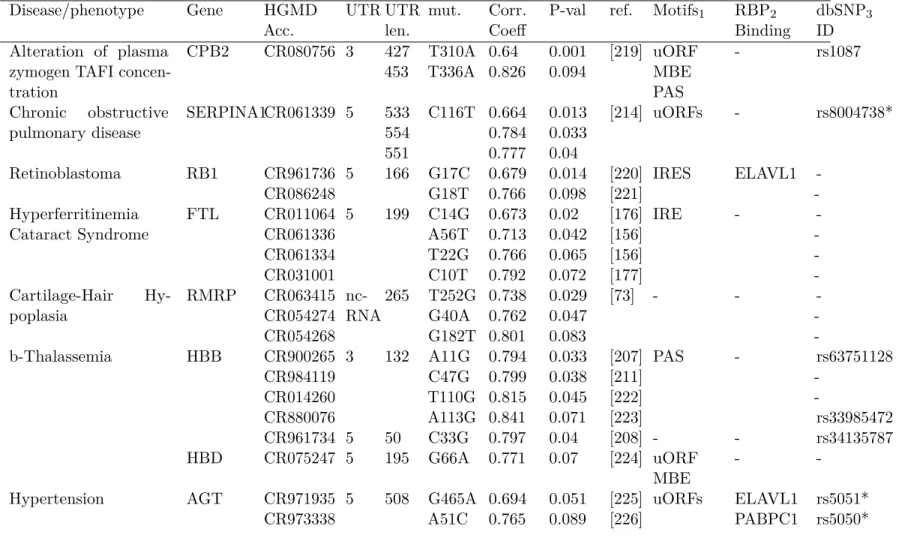
2.1 Disease states and phenotypes in which two or more associated SNPs significantly alter structure . . . 67
2.2 Relative population of the three structural clusters for the FTL 5’ UTR . . . 70
2.S1 Disease states and phenotypes in which one associated SNP was found to alter the structural ensemble of the RNA. . . 80
2.S2 Comparison of SNPfold scores in pre- and mature mRNA 5’ UTRs . . . 81
2.S3 eQTL data for common variant SNPs identified as potential RiboSNitches . . . 82
3.1 Structure stabilizing haplotypes in the human genome where more than four SNP pairs stabilize RNA structure. . . 97
3.S1 SNPfold predicted secondary mutations to correct the U22G hyper-ferritinemia associated SNP . . . 106
3.S2 SNPfold predicted secondary mutations to correct the A56U hyper-ferritinemia associated SNP . . . 107
3.S3 Full list of structure-stabilizing haplotypes in the human genome . . . 109
4.1 SNRNASM assays currently in OBI along with their corresponding Probes . . 130
5.1 Putative RiboSNitches caused by eQTL SNPs proximal to RBP binding sites . . . 150
5.S1 SNP dataset statistics . . . 158
5.S2 PAR-CLIP statistics . . . 159
5.S3 SNPfold analysis results for SNPs near C22ORF28 . . . 160
5.S4 SNPfold analysis results for SNPs near ELAVL1 . . . 161
5.S5 SNPfold analysis results for SNPs near FXR1 . . . 165
LIST OF FIGURES
1.1 An example of a theoretical riboswitch . . . 7
1.2 Chemical structure of RNA and its nitrogenous bases . . . 18
1.3 Simple structural motifs that are common components of full
sec-ondary structures of RNAs . . . 21
1.4 The Nussinov algorithm . . . 24
1.5 Main recursions utilized by the Zuker and MacCaskill algorithms . . . 33
1.6 An example of two RNAs with divergent sequence content but
conserved structure . . . 46
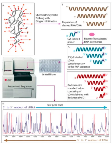
1.7 General workflow for a chemical mapping experiment utilizing a
capillary electrophoresis machine . . . 48
1.8 Events that mRNA is subject to that are dependent on binding
affinity with protein and other RNAs . . . 53
2.1 Partition function analysis of the C33G SNP in the 5’ UTR of HBB
associated withβ-Thalassemia. . . 63
2.2 Comprehensive single mutation analysis of the HBB 5’ UTR to
determine the significance of mutation RNA structure change . . . 65
2.3 Principal Component Analysis of structural ensembles from FTL 5’
UTR mutations . . . 69
2.S1 Principal component decomposition of Boltzmann sampling of the
RB1 5’ UTR . . . 78
2.S2 Average change in in FTL 5’ UTR basepairing probabilities due to
Hyperferritinaemia Cataract Syndrome mutations . . . 78
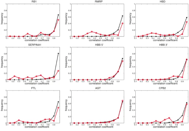
2.S3 Comparison of WT/SNP correlation coefficient distributions for all
possible mutations in riboSNitch-containing UTRs . . . 79
2.S4 Comparison of WT/SNP correlation coefficient distributions for all
possible mutations in riboSNitch-containing UTRs . . . 83
2.S5 pre-mRNA gene maps of SNPs that are in high LD (R2 >0.9) with
our predicted RiboSNitch SNPs . . . 86
3.1 A principal component decomposition of Boltzman sampled sub-optimal structures for wildtype and Hyperferritinemia Cataract
3.2 Results of SHAPE experiments conducted on FTL 5’ UTR sequence variants 93
3.3 SHAPE analyses of compensatory mutations in the mutated FTL 5’
UTR selected to restore structure . . . 95
3.4 A structure stabilizing haplotype identified in the 3’ UTR of RPA1
using SNPfold analysis . . . 98
3.S1 SHAPE analyses of multiple mutations and sequence variants in the
FTL 5’ UTR . . . 105
3.S2 Distribution and thresholding of structure recovery ratios . . . 108
4.1 Different possible scenarios for SNRNASM data . . . 128
4.2 Tree representation of nucleic acid structure probing terms added to OBI . . . . 131
4.3 Example meta-analysis of DMS chemical mapping data from two
separate studies on RNA . . . 136
4.S1 Evidence of SNRNAM’s ability to differentiate chemical and
enzy-matic probing . . . 139
4.S2 Example of an ISA-Tab file . . . 140
5.1 Possible mechanisms by which a SNP can affect RNA/protein
inter-actions, and examples of overlap . . . 143
5.2 Transcriptome coverage analysis of PAR-CLIP and eQTL SNP data sets . . . . 146
5.3 direct and proximal overlap enrichment/depletion of
SNP/PAR-CLIP clusters in human 3’ UTRs . . . 148
5.4 Effects of eQTL SNPs proximal to RBP binding sites on 3’ UTR
structural ensemble for two representative UTRs . . . 152
6.1 A scanning of the entropy per unit energy along the FTL 5’ UTR . . . 179
6.2 Structural elements conserved across species with evidence of
LIST OF ABBREVIATIONS
AUC Area Under the Curve CC Correlation Coefficient CDS Coding Sequence DMS DiMethyl Suffate
eQTL expression Quantitative Trait Locus FN False Negative
FP False Positive FTL Ferritin Light Chain
GWAS Genome-Wide Association Study HGMD Human Gene Mutation Database IRE Iron Response Element
ISA Investigation/Study/Assay
IREBP Iron Response Element-Binding Protein ISA Investigation/Study/Assay
LD Linkage Disequilibrium MFE Minimum Free Energy MI Mutual Information mRNA mature RNA
NMIA N-MethylIsotoic Anhydride
OBI Ontology of Biomedical Investigation
PAR-CLIP Photoactivatable-Ribonucleoside-Enhanced Crosslinking and Immunoprecipitation PCA Principal Component Analysis
ROC Receiver-Operator Curve RNA RiboNucleic Acid
RT Reverse Transcriptase
SHAPE Selective 2’-Hydroxyl Acylation followed by Primer Extension SNP Single Nucleotide Polymorphism
SRP Signal Recognition Particle SRR Structure Recovery Ratio SSH Structue Stabilizing Haplotype TN True Negative
TP True Positive
CHAPTER 1 Introduction
1.1 Unexpected results from GWAS and transcriptome profiling challenge be-liefs on the function of RNA
At around the same time, the functional status of these intergenic regions was coming under question due to large-scale tiling arrays being carried out in order to determine just how much of the human genome was being transcribed. Initial estimates from the pilot phase of the ENCODE project using tiling arrays showed that upwards of 93% of the genome was in some way, shape or form transcriptionally active [11, 12]. Due to the shortcomings of utilizing tiling arrays, such as the significant distances in the genome between probe-covered sites and the inability to ascertain the abundances of transcripts, these initial results were subject to scrutiny and debate [13]. In the follow-up phase to the ENCODE project, concerns over the accuracy of the conclusions reached from tiling arrays were addressed by utilizing RNA-seq instead to determine both transcription coverage and transcript sequence. Results from this study dropped the percentage of the genome reported to be transcriptionally active down to 74.7% [14]. Technology now exists to specifically target transcripts produced from the so-called intergenic regions, and has been used to uncover low abundance transcripts that show evidence of undergoing processing [15]. From these results it is clear that much more of the genome is transcriptionally active than once thought. Given the number of trait or disease-associated SNPs found in untranslated or intergenic loci in the human genome, combined with the strong evidence that the majority of the human genome is passed on to an RNA transcript, it seems reasonable to assert that a number of functional SNPs being tagged in genome studies (including those that fall in supposedly gene-bare areas) are in regions that are transcribed but not translated, and that they exert their effect by altering RNA transcript functionality or regulation.
1.2 Our initial understanding of RNA’s biological function
proteins; Beadle and Tatum, through mutational analyses of Neurospora crassa, found mutant strains that required particular vitamins for growth, and that the enzymes normally responsible for the production of these vitamins had acquired a genetic defect [16]. Later work done after the discovery of DNA cemented RNA’s important role in protein production. Crick et al. discovered through mutational studies of genes in T4 virus that the insertion or deletion of a single nucleotide can completely abolish could lead to a complete loss of protein function. In further experimentation they found that exposing these mutant strains to an additional round of mutagenesis could restore the function, and that the locations of compensatory mutations were usually very close to that of the original insertion/deletion mutation [17]. In the early 1960s, Nirenberg et al. not only deciphered the triplet genetic code alluded to by Crick, but also confirmed RNA’s essential as the intermediate carrier of the information required for protein synthesis. To do this, Niremberg and his colleagues took advantage of cellular extract from bacteria, known to still be able to synthesize protein even after cell lysis. They applied DNase, which degrades any DNA present, and then added synthetic RNA of known sequence content to the extract. Not only did they observe that protein product now occurred, but also, by controlling the nucleotide content of poly(GU) input RNA so that GGG was the most likely triplet they were able to confirm that in RNA, a triplet sequence codes for an amino acids. Through the application of this method using RNA polymers and labeled amino acids in the extract, the specific amino acid produced by each triplet codon was deduced [18]. Other important roles of RNA in this process, known as translation, were being discovered at the same time : Chapeville et al. discovered that tRNAs with sequence complementarity to each triplet carry the corresponding amino acid, and multiple scientists identified the large RNAs that formed the scaffold for the prokaryotic and eukaryotic ribosomes [19, 20].
within the cell. later work, however, would reveal that the diversity of functions of RNA had been underestimated.
1.3 RNA’s full range of functionality begins to be understood
Research on the function of RNA in the years since the cracking of the codon code and the deduction of RNA’s role in protein production has revealed that RNA is not merely the carrier of blueprints for proteins. Like DNA and proteins, it can be modified in ways that affect its function. And like proteins it can catalyze reactions and respond to the presence of small molecules. Over time RNA has proven to be a multifunctional biomolecule whose activity has proven essential for multiple forms of gene regulation in the cell.
Splicing was first discovered in the late 1970s by the labs of Richard Roberts and Phillip Sharpe in their studies on RNA transcripts from Adenovirus. Here, they experimentally showed that a single Hexon mRNA produced by Adenovirus consisted of sequence correspond-ing to four discontiguous regions of the Adenovirus genome, providcorrespond-ing electron microscopy images of a DNA fragment from the Adenovirus genome hydrogen-bonded via small stretches of sequence to the Hexon mRNA, separated by large loops [21, 22]. Further research into the transcripts produced by Adenovirus showed that several different transcript isoforms can be mapped to these transcribed regions of the Adenovirus genome, indicating that a so-called gene region in the DNA of an organism can produce via alternative splicing multiple distinct transcripts. This phenomenon has been shown to be extremely common in eukaryotes, especially those that are higher-order organisms where the presence of multiple tissue types dictates that it is important to have tight control over gene regulation: vertebrates have been shown to have a considerably higher portion of transcripts that where alternative splicing occurs than invertebrates [23, 24].
are often subject to direct chemical alteration or modification as well. There are currently on record from the RNA Modification database (mods.rna.albany.edu/) 109 distinct distinct modified nucleosides that have been detected in some RNA. The class of RNA with the largest number of these modified nucleotides is tRNA, with 95 of these modification events being detected at some point (a statistic taken frommods.rna.albany.edu), and an average of eight nucleotides being found in each tRNA molecule [30]. These many modifications serve various roles, including the promotion of proper codon-anticodon interactions, increasing stability by lowering the free energy of the tRNA structure, and acting as a form of identification for particular tRNAs in the cell [31–36]. Other RNAs that are well known as targets of nucleotide modification are rRNA and snRNA, with both undergoing modifications serving the purpose of enhancing functionality either through an increase of structural stability or the promoting of particular hydrogen bond interactions with other biomolecules [37]. There have also been multiple modification events detected in eukaryotic mRNAs, the most famous and well known being a C-to-U editing event in the gene APOB which leads to a premature stop codon, altering the final protein product produced by the APOB mRNA [38]. Both C-to-U and A-to-I editing events have been observed in eukaryotic mRNAs. The A-to-I events are far more common, and are believed to serve multiple functions, including the modification of anti-codon wobbles (where the Inosine gets misread as a Guanosine) and the modification of miRNA functionality [31, 39]. These particular modifications have also been shown to preferentially occur in structured double-stranded RNA elements typical of transcribed retrotransposons and foreign RNA [40]. It is believed that this editing event plays a particularly important role in brain tissue, where significantly higher rates of A to I editing have been reported than in other assayed tissues [41–43].
any other cellular enzyme or RNP [44]. Altman and colleagues, in their work with the RNP known as RNase P, showed that under in vitro conditions the RNA component of RNase P is capable of catalytically processing tRNA precursor transcript in the absence of its protein partner, leading to the conclusion that the RNA component of this RNP was the component responsible for its catalytic activity [45]. Since these discoveries multiple additional enzymatically active RNAs, now known as ribozymes, have been made. Many more examples of independently functioning self-splicing introns like that within the rRNA ofTetrahymena have been found in transcripts from other organisms, leading to this form of intron being given its own classification, the group I self-splicing intron. Another class of catalytic intron, known as the group II intron, displays a similarity to RNase P activity in that it is able to catalyze its splicing reaction alone in particular conditionsin vitro. Both group I and group II introns can be found across multiple kingdoms of life. There are other examples of ribozymes, including the hammerhead ribozyme, which consists of a structural motif that catalyzes a single nucleotide backbone cleavage event in itself, and the Hepatitis D virus ribozyme [46, 47].
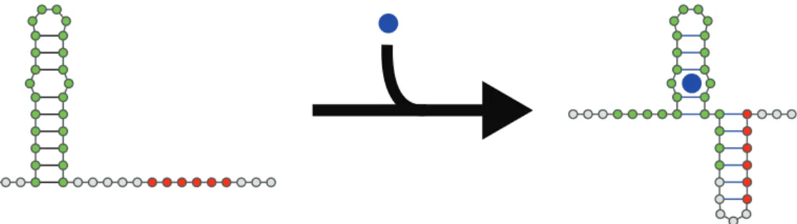
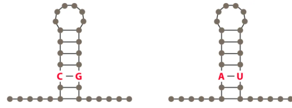
Figure 1.1: An example of a theoretical riboswitch. The region in green is the aptamer, or the part of the riboswitch that binds some small molecule, while the region in red is an expression platform, or some important functional sequence. When the small molecule is introduced (or more realistically, when it reaches a certain physiological concen-tration) the riboswitch undergoes a conformational change such that the expression platform is rendered inaccessible, altering gene regulation and expression. Structures generated using VARNA [48].
nucleotide to rearrange the structure of an RNA is a central focus of this work, and this riboswitch will be a point of reference in later chapters.
The work described in the last few decades has led to a general paradigm shift in the genetics and Molecular Biology community, with respect to how they view the role of RNA in the cell, from that of a general carrier of protein-coding information to a multifunctional biomolecule capable of being highly regulated, catalyzing reactions and reacting to changes in physiological state within the cell. These findings, as well as additional findings from the past decade, lead to our current understanding of the extent of the roles that RNA plays within the cell.
1.4 The many different classes and functions of RNA in the cell
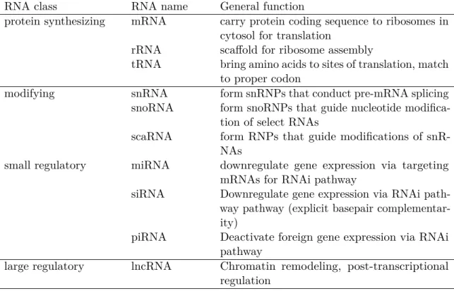
Many of the types of functional RNA that were initially found in the cell were directly involved in protein synthesis. Over time, however, a broad variety of RNAs across different kingdoms of life have been discovered that play important roles in all sorts of known cellular processes, including post-transcriptional gene regulation, splicing, immune response and ribonucleoprotein assembly (Table 1.1).
1.4.1 Classes of RNA involved in protein synthesis
new alternative ways of processing information in existing genes than it is to inherit entirely new genes over time. This class of RNA is essentially ubiquitous across all organisms, since all known forms of life need to be able to be able to synthesize protein using ribosomes and transfer instructions for production of protein to progeny. The second class of RNA discovered is ribosomal RNA (rRNA), which forms part of both small and large ribosomal subunits across the kingdoms of life. Ribosomal RNA acts as the primary determinant of the folded structure of the ribosome, acting as a scaffold to which multiple proteins bind to during its assembly. In fact, the majority of the final structure is taken up rRNA; the ribosome is stabilized by tertiary interactions between its rRNAs’ secondary structure domains, as well as the binding of multiple proteins to the both the rRNA surface and exposed pockets [61]. The third discovered class of RNA discovered is tRNA, which brings the amino acid corresponding to a particular codon to the growing nascent polypeptide chain during translation so that it can be added. As mentioned before, a tRNA molecule that is meant for a particular codon has base complementarity to that codon in the anticodon loop of its folded structure, and often contains many modification that serve the purpose of promoting stability, as well as allowing other cellular machinery to identify the tRNA. While these classes of RNA are well studied and essential to every organism one way or another, they only scratch the surface of the many types of RNA that can be found within cells.
1.4.2 RNAs that guide post-transcriptional modification events
RNA class RNA name General function
protein synthesizing mRNA carry protein coding sequence to ribosomes in cytosol for translation
rRNA scaffold for ribosome assembly
tRNA bring amino acids to sites of translation, match to proper codon
modifying snRNA form snRNPs that conduct pre-mRNA splicing snoRNA form snoRNPs that guide nucleotide
modifica-tion of select RNAs
scaRNA form RNPs that guide modifications of snR-NAs
small regulatory miRNA downregulate gene expression via targeting mRNAs for RNAi pathway
siRNA Downregulate gene expression via RNAi path-way pathpath-way (explicit basepair complementar-ity)
piRNA Deactivate foreign gene expression via RNAi pathway
large regulatory lncRNA Chromatin remodeling, post-transcriptional regulation
Table 1.1: Known classes of Eukaryotic RNAs separated by their function.
OH methylation events, primarily acting on snRNAs and localizing to an snRNP processing-focused compartment in the nucleolus known as the cajal body [67]. There are additional RNAs involved with transcript modification that are difficult to place into a particular class. RNase P, previously referenced as one of the first ribozymes discovered, makes up part of an RNP that splices pre-tRNA transcripts into tRNAs. The RNA component of telomerase helps prime the extension of telomeres, elements at the end of chromosomes that protect from DNA decay via free radicals, via a mechanism dependent on the RNA’s tertiary structure [68, 69]. RNase MRP makes up part of an RNP, and has multiple roles, including the priming of mitochondrial DNA during transcription and involvement in the production of siRNA [70, 71]. This particular RNA will be of interest to us in later chapters when we analyze the structural basis of mutations in it that are associated with the genetic disorder cartiliage-hair Hypoplasia [72, 73].
1.4.3 Gene regulatory RNAs
An additional broad set of identified RNAs serve the function of regulating gene expres-sion. Here, there is a particularly wide variety of different RNAs with different transcript characteristics and mechanisms of function. It would be simplest here to separate these gene regulatory transcripts into two groups: small RNAs and larger RNAs.
1.4.3.1 Small regulatory RNAs
1.4.3.2 Large regulatory RNAs
modulation of chromatin state in order to control transcription. A well known lncRNA that uses this mechanism is HOTAIR, which is able to silence transcriptionally active sites in the genome by recruitment of an RNP known as the Polycomb Repressive Complex (PRC) at sites in chromatin, where it conducts H3K27 trimethylation in order to promote a closed chromatin state [88, 89]. In general, lncRNAs exert control over chromatin state by either altering the activity of chromatin-regulating proteins in a promoting or repressive manner. Many examples of known functional lncRNAs that regulate gene activity via chromatin modification exist [88, 90, 91]. There is also evidence of some lncRNAs controlling the recruitment of transcription initiation factors to promoter regions [92, 93]. Additionally, examples exist of lncRNAs regulating gene expression post-transcriptionally through various means, including altering splicing, being processed into endogenous siRNA, and the control of translational efficiency [94–96].
1.5 The chemistry of RNA
While the wide diversity of functions that RNA is involved in should now be clear, it is also very important to discuss reasons for which RNA is able to take on so many role in the molecular biology of organisms. The chemical properties of RNA enable fast, direction-specific, energy-efficient synthesis via polymerization, as well as the ability contain a variety of function-specific information within its sequence made primarily of an alphabet of 4 characters. The chemistry of RNA also allows it to form structures that can make it possible for the RNA to interact with other molecules both small, and in some cases enable the formation of an active site in the RNA that can catalyze reactions. Ultimately, it is the chemistry of RNA that determines its function.
1.5.1 General chemistry of biopolymers
a polymer consists of monomer compounds that are covalently bonded together to form repeating units.
In many cases of biopolymers, the chemical composition of each monomer is identical. This is the case with polysaccharides, where the monomer is an aldehyde or ketone with at least two hydroxyl groups (and thus at least 3 carbons forming its backbone). Simple polymers can have a structure supporting role (chitin, cellulose) or an energy storing role (starch, glycogen) in the cell [16]. The structure-supporting polysaccharides involve long linear chains of monomer units (with cellulose and chitin the monomers are glucose-derived units covalently linked viaβ 1,4 glycosidic linkages). The energy storing polysaccharides can come in linear or branched form. The amylose portion of starch is linear, linked via
α 1,4 linkages, whereas glyocogen and the amylopectin portion of starch contain both α
1,4 andα 1,6 linkages) [97]. Synthetic polymers also usually consist of simple homogenous monomers, as this lends itself to predictable, stable polymer chemistry. However, for the transfer of information and reaction catalysis that is necessary for the sustaining of life, it is insufficient. For this, there needs to be an increased level of complexity in the monomeric units that make up biopolymers.
In order to take on high level structure and more diverse functionality, other proteins like polypeptides and nucleic acids have side groups that are part of each monomeric unit. In proteins, the monomeric unit, the amino acid, is a simple organic compound, consisting of a positively charged amino group and a negatively charged carboxyl group joined together via anα carbon at the center. It is the R-group side chains that are also attached to the
or RNA) are identical, save for the ”side group” nitrogenous base. The alphabet of ”side group” bases in nucleic acid polymers is much smaller than in proteins, as well as far less reactive. Because of this nucleic acids are significantly less catalytically active. An additional important distinction to make between proteins and nucleic acids is that the synthesis of nucleic acids is far less energetically expensive than proteins [97]. Taking these factors into consideration it seems logical that in organisms nucleic acids are more likely to be carriers of information, while proteins are more likely to be involved in enzymatic activity necessary for biological function. As nucleic acid biochemists and RNA biologists have found out, however, the truth is not so black and white.
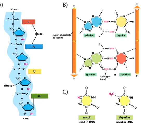
1.5.2 The chemistry and primary structure characteristics of DNA and RNA DNA, the classical nucleic acid polymer, has several features that make it particularly well suited for information transfer. Its 2’ Carbon in its central ribose ring lacks a hydroxyl group that is typically found in a ribose sugar. This protects the phosphate backbone from being nucleophilically attacked by the 2’ hydroxyl group, a common spontaneous occurrence in nucleic acid polymers with this group on their ribose sugar. More importantly, DNA comes double-stranded, with strands running antiparallel and reverse complementary to one another. This strand complementarity allows for polymer-wide canonical Watson-Crick basepairing between nucleotides on opposite strands (3 hyrdogen bonds between Guanine and Cytosine bases, 2 hyrdogen bonds between Adenine and Thymine nucleotides) [98]. This double-strandedness provides increased protection from degradation, and also makes the process of replicating DNA particularly effective, with two double-stranded DNAs (each containing a parent strand of DNA) being produced from an individual double-stranded DNA replication event. The fact that each daughter dsDNA has a single parent strand is advantageous for detecting replication errors or spontaneously altered bases, as this can result in basepair mismatches in the dsDNA that can be detected and repaired by DNA repair enzymes [16]. DNA is well adapted to the role of carrying gene information and passing it on to daughter cells via its replication.
A)
B)
C)
Figure 1.2: Chemical structure of RNA and its nitrogenous bases. A) A schematic figure representing the backbone of a nucleic acid biopolymer. This particular nucleic acid is RNA, since it has at every ribose 2’ position a Hydroxyl (OH) group, whereas in DNA this group is not found at this position. B) The general hydrogen bonding between bases seen in nucleic acids. Guanine and Cytosine (seen in both DNA and RNA) bond via three hydrogen bonds, whereas Adenine and Thymine (found in DNA) form two basepairs.C) In RNA that has been transcribed from DNA, Uracil replaces Thymine. Uracil forms two hydrogen bonds with Adenine, and can also interact via two hydrogen bonds with Guanine. Adapted from [16]
nitrogenous bases found in RNA, the Thymine typically found in RNA is replaced with Uracil in RNA. A possible explanation for why DNA might use Thymine as a base instead of Uracil is that Cytosine deamination is a common mutagenic event that requires repair, and that a Cytosine, when deaminated, becomes a Uracil. DNA repair mechanisms, when searching for these Cytosine deamination events likely would have a large amount of difficulty telling the difference between natural Uracils and deaminated Cytosines, and for this reason Thymine, chemically equivalent to 5-methyluracil, or a Uracil base with a methyl group added at the fifth position of the base’s aromatic ring, is used instead.
In spite of the fact that these characteristics that seem to do little more than confer instability, the fact that RNA typically is single-stranded allows it take on higher order structure that DNA is too structurally constrained to form. This structure plays a key role in RNA’s ultimate set of functions in nature.
1.5.3 Higher-order structure
Like other polymers with differential compositions of monomers (the best examples being the aforementioned DNA and protein) RNA is governed by thermodynamic laws that cause it, from its linear, unfolded state, to seek a lower free energy status by folding into a more energetically stable conformation. While this issue does not concern DNA, due to its high stability through maximized basepairing with a complementary strand, RNA sequences, like protein, are under thermodynamic pressure to fold in a way that minimizes their free energy.
1.5.3.1 A comparison of folding in proteins versus RNA
protection from polar water molecules can be found. Analogously, a large driver of RNA folding is the thermodynamic pressure to lower the free energy of the polymer by burying hydrophobic nitrogenous bases in basepairs. With respect to secondary structure formation, both proteins and RNA rely on hydrogen bonding interactions. However, proteins rely on interactions between parts of their monomeric units, not even involving their side chain groups, which are more involved in tertiary structure formation. The motifs formed in proteins are rather ubiquitous, involving interactions between Amino and Carboxyl groups of amino acids to form well defined secondary motifs such as the α helix or theβ pleated sheet [97]. In RNA, the secondary structure primarily consists of canonical Watson-Crick pairing between nitrogenous base ”side groups”. With respect to tertiary structure, both protein and RNA contain common motifs amongst themselves. In protein, the side groups are the primary determinant of tertiary structure, whereas in RNA, the secondary structures formed are key determinants of the tertiary structure (often formed as a result of their interactions). While the formation of protein secondary structure and tertiary structure are not thought to be particularly independent of one another, it is known that a majority of an RNA structure’s stability comes from the basepairing inherent to its secondary structure [99, 100].
1.5.3.2 RNA secondary structure
paradigm becomes more relevant once energy parameters from experimentation are brought into RNA secondary structure prediction.
Bulge Stem Loop
Multi-branched Loops Stem
Internal Loops
Single-stranded
A)
Pseudoknot Kissing Stemloop
B)
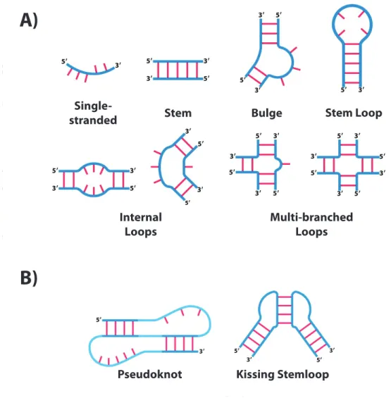
Figure 1.3: Simple structural motifs that are common components of full secondary structures of RNAs. A) Structural motifs that utilize non-overlapping basepairing, where givenij and hkbasepairing, h < i < j < k. In present secondary structure prediction methodologies, thermodynamic parameters for these motifs (in particular, ones including the stem motif, where consecutive basepairs add additional stability) have been defined via physical chemistry experimentation. B) Structural motifs where theh < i < j < kdoes not hold. While these motifs are known to be relatively common in structured RNA, the computational complexity involved in their prediction has made it difficult to integrate their detection into structure prediction algorithms. Adapted from [16]
1.5.3.3 RNA tertiary structure
While often RNA is depicted as only folding on a two-dimensional plane, there is an additional dimension of folding that takes place, compacting a transcript further into its folded structure. The tertiary structure of an RNA will often involve a mixture of canonical Watson-Crick and noncanonical base interactions between secondary structural elements formed. Just as the secret to stable secondary structure in RNA lies in the stacking of consecutive basepairings to form stems, in tertiary structure, stacking of stem regions of folded RNA provides a great deal of additional stability, and has been found to be common in tertiary structures of structurally conserved RNAs, with a perfect example being the stacking of the stem regions in tRNA [16]. There are also particular motifs in tertiary structures that confer additional stability. The pseudoknot and kissing loop motifs can be considered tertiary interactions since they do not really operate on a two-dimensional plane (Figure 1.3B). Another motif, the tetraloop, is found in loop regions in secondary structures, and involves interactions between the four nucleotides that involve a non-planar structural representation [102]. Such a motif is actually regularly incorporated into the calculation of energies for secondary structure prediction programs [103]. Additionally, a motif known as a G-quadruplex uses non-canonical interactions between four consecutive Guanine residues to provide stability, and has been found to be biologically functional in different scenarios at both the DNA and RNA level [104]. Algorithms now exist that allow for its detection in RNA structure prediction, and interestingly their presence is observed to be enriched in 5’ UTRs of mRNAs [105].
1.6 RNA Secondary structure prediction
The accurate prediction of secondary structure of RNAs has been a popular research topic in computational biology for several decades. Because of the large number of described basepairs that are possible for a given sequence, there are a myriad number of possible secondary structures that a transcript can adapt, with an estimate of 1.8N possible secondary
structures, given a sequenceN nucleotides in length [108]. While for some small RNAs it is possible to make an accurate guess at the most stable RNA secondary structure that can be formed, it is typically impossible to determine without the use of some sort of scoring which structure of the many that are possible for a sequence is the most likely to be found in solution. The history of research into answering this question will now be reviewed.
1.6.1 The Nussinov algorithm
One of earliest attempts at predicting the secondary structure for an RNA given its primary sequence came from Nussinov and colleagues in the late 1970s [109]. Attempts had been made before to create means of predicting the optimal structure for a given sequence, but they involved algorithmic approaches that were somewhat inefficient and took an unreasonable amount of time to run [110]. The Nussinov algorithm seeks to find the most likely structure in a more efficient manner through the use of dynamic programming. Dynamic programming is a method that can be used to solve a complex problem in a time efficient manner. It does this by breaking down a given problem into the smallest possible subproblems, building off of the answers to these subproblems to eventually arrive at the optimal solution to the overall problem in question. Here, the explicit problem that the Nussinov algorithm seeks to answer is to identify the secondary structuresfrom a collection of possible secondary structuresS with the maximum number of basepairings b. To put this in more mathematical terms, the goal of the algorithm is to find :
A)
i i+1 j j-1 ij basepair i i+1 j i unpaired j j-1 i j unpaired j i k k+1 bifurcationB)
G G G G A A A C C C CG 0 G 0 0
G 0 0
G 0 0
A 0 0
A 0 0
A 0 0
C 0 0
C 0 0
C 0 0
C 0 0
G G G G A A A C C C C G 0 0 0 0 0 0 0 1 2 G 0 0 0 0 0 0 0 1 2 3
G 0 0 0 0 0 0 1 2 2 2
G 0 0 0 0 0 1 1 1 1
A 0 0 0 0 0 0 0 0
A 0 0 0 0 0 0 0
A 0 0 0 0 0 0
C 0 0 0 0 0
C 0 0 0 0
C 0 0 0
C 0 0
G G G G A A A C C C C G 0 0 0 0 0
G 0 0 0 0 0 0
G 0 0 0 0 0 0
G 0 0 0 0 0 1
A 0 0 0 0 0
A 0 0 0 0 0
A 0 0 0 0 0
C 0 0 0 0 0
C 0 0 0 0
C 0 0 0
C 0 0
G G G G A A A C C C C G 0 0 0 0 0 0 0 1 2 3 4 G 0 0 0 0 0 0 0 1 2 3 3
G 0 0 0 0 0 0 1 2 2 2
G 0 0 0 0 0 1 1 1 1
A 0 0 0 0 0 0 0 0
A 0 0 0 0 0 0 0
A 0 0 0 0 0 0
C 0 0 0 0 0
C 0 0 0 0
C 0 0 0
C 0 0
G G G G A A A C C C C G 0 0 0 0 0 0 0 G 0 0 0 0 0 0 0 1
G 0 0 0 0 0 0 1 2
G 0 0 0 0 0 1 1
A 0 0 0 0 0 0 0
A 0 0 0 0 0 0 0
A 0 0 0 0 0 0
C 0 0 0 0 0
C 0 0 0 0
C 0 0 0
C 0 0
G G G G A A A C C C C G G G G A A A C C C C
C)
G G G GA A A
C
C
C
C
Figure 1.4: The setup and execution of the Nussinov algorithm.A) The possibilities for basepairing in the structure
Sgiven nucleotidesiandj.B) A walkthrough of the filling in of the dynamic programming array used in the Nussinov algorithm. The array is first initialized by setting every position in the matrix wherei=j ori−1 =j to 0. The matrix is then filled along the diagonal, inputting in each space a value forbconsistent with which of the four types of possibilities fromAwould produce the maximumbvalue. The final array depicts the traceback step, where theij
indeces are sent back through filled in values in order to yield the path consistent with a structure or structures for the input sequence that have the number of basepairingsbmax.C) The single structure emitted by the input sequence
with the number of basesbmax, obtained from traceback. Structures generated using VARNA [48].
Assuming that the ensemble of possible structures S is generated from a sequence X, where X is N characters in length and X = (x1, x2, ..., xN), the Nussinov algorithm calls
initialized to 0. In the filling of this matrix, we consider four possible scenarios: a direct
ij basepairing, an unpairedi, an unpairedj and a bifurcation loop where iandj are the outermost nucleotides (Figure 1.4A). From here,γ is filled using the following recursion:
for i = 2 to Ndo forj = i to N do
w=
1 X[i] and X[j] are canonical bases
0 otherwise
γ[i, j] = max
γ[i+ 1, j]
γ[i, j−1]
γ[i+ 1, j−1] +w
maxi<k<j(γ[i, k] +γ[k+ 1, j]) end for
end for
At the final position inγ that is filled (γ[1, N]), the value stored is equal to the maximum number of possible basepairsbmax for any of the possible structures inS. From this position
in the matrix, it is now necessary to conduct a traceback in order to determine the structure that is compatible withbmax. To do this, the following recursion back through the matrix
applies:
i= 1;j=N;
while i < N and j >1 do if γ[i+ 1, j] =γ[i, j]then
i=i+ 1
else if γ[i, j−1] =γ[i, j]then
j =j−1
else if γ[i+ 1, j−1] +w=γ[i, j]then Store basepairing in X betweeni,j i=i+ 1
else
for k=i+ 1 toj−1do
if γ[i, k] +γ[k+ 1, j] =γ[i, j]then
i=k+ 1
j=k
end if end for end if end while
After running this traceback through γ, A series of basepairings are generated, creating a secondary structure whose number of basepairings is equal to bmax. An illustration of
this algorithm being utilized on an RNA sequence GGGGAAACCCC has been provided (Figure 1.4B). In this example we see that the traceback yields abmax of 4, and ans(bmax)
consisting of a stemloop with four basepairs and a loop region of three nucleotides (Figure 1.4C). The filling of γ is O(N3) in runtime and O(N2) in required memory, whereas the traceback operation is O(N) in runtime and required memory [109].
While this algorithm was a pioneer with respect to setting up a method of predicting RNA secondary structure in an efficient manner, there were also several disadvantages to its approach, mainly centering around the incongruity between its approach and the actual thermodynamics of RNA structure. Perhaps the largest issue with the Nussinov algorithm is that the assumption that the structure with the maximal amount of basepairs is the most stable structure in the RNA is flawed. As alluded to before, while it is true that lower free energy structures are more likely to have a large amount of basepairs, the orientation of these basepairs is critically important, due to the additive stabilizing effect on dsRNA regions that consecutive basepairs offer [111]. Because of this, just because a structures
has a number of possible basepairs bmax, doesn’t mean that it has the lowest possible free
energy structure in the ensemble of possible structuresS. Another flaw that can make itself evident in the traceback step is that there are sequences that emit from S more than ones
accurately represents a method to access a set of structures {s1, ..., sn:s∈S;b(s) =bmax}.
This method allows for a decent guess at the lowest energy structure within S, particularly in RNAs that are where there is a strong predominant structure such as in tRNAs. However, a more accurate identification of the lowest free energy structure within the ensemble of possible structures S requires the use of specific thermodynamic parameters as guidance, rather than the number of basepairings b.
1.6.2 Thermodynamic parameters of RNA secondary structure obtained through experimentation
When finding the lowest free energy structuresin the structural ensembleS of a sequence
X, the value used as a measurement of this energy is commonly known as Gibb’s Free Energy. For a given state, the Gibb’s Free Energy is defined as the difference between the Enthalpy of the state in question and its temperature-adjusted entropy. Or, put differently,
G=H−T S
Where G is the Gibb’s Free Energy, H is the Enthalpy and S is the entropy (not to be confused with the S being utilized before the represent an ensemble of structures). Here, we wish to look at the change in Gibb’s Energy when a particular structure forms, under the conditions of a constant internal environment (constant volume and pressure). Therefore we use the equation
H =U +P V
where U is the internal energy of the system andV is the volume, to modify the equation to
dG=dU+P dV +V dP −SdT −T dS
Where T is the temperature within the system. We can then use the equation
To substitute in for dU, in order to get
dG=V dP −SdT
To estimate the change in Gibb’s Free Energy that occurs when an RNA folds, the general strategy utilized is to calculate the energetic contributions of RNA/RNA duplex formations that make up a structure that make up a particular structure s. To facilitate understanding we will consider the following example, where GG and CC dinucleotides are ”reactants”, and a GG/CC duplex is the ”product” (though there is no actual modification
of any of the reactants’ chemistry). In a situation where GG and CC basepair:
GGss+CCssGG/CCds
We wish to find some way to calculate thedGfor such a reaction. To approach this problem we alter our equation for Gibbs Energy by adding additional terms µCC,µGG andµCC/GG
representing the chemical potential inherent to a reactant or product, or the following:
µi =
∂G
∂ni
T,P,n¬i
Where the termni is the molar quantity of itemi, andn¬i refers to the molar quantities of
any item that is noti. Given these added terms, a non-constantni, and constantT and P,
our new equation is
dG=µGG∗dnCC+µGG∗dnGG+µCC/GG∗dnCC/GG
Given that the change in the amount of reactant is represented by dnCC anddnGG, and the
amount of product is represented by dnCC/GG, we introduce a new term dξ that is equal
nreactant and positivenproduct,
dξ=−dnreactants=dnproducts
We substitute this equation into our terms for dGto get
dG= (µproducts−µreactants)dξ=
µCC/GG−(µCC+µGG)
dξ
and
∂G
∂ξT ,P =µproducts−µreactants=µCC/GG−(µCC +µGG)
From here we can apply ideal gas laws to each µi, such that
µi=µ0i +RT ln(Pi/1atm)
to get
∂G
∂ξ
T ,P
=hµ0products+RT ln(Pproducts/1atm) i
−hµ0reactants+RT ln(Preactants/1atm) i
or simplified,
∂G
∂ξ
T ,P
=dG0+RT lnPproducts Preactants
=dG0+RT lnPCC/GG PCCPGG
Since we are dealing with oligonucleotides in solution we can deal with molar concentrations, rather thanP for each item. Also, if we look atdG0 when−µreactants=µproducts, we are
looking at the equilibrium state where subsequently∂G∂ξ
T,P = 0. Thus,
dG0 =−RT ln[CC/GG]
[CC][GG] =−RT lnKp
Where Kp is the equilibrium constant of the reaction in question. Lastly, we can take an
and Gibbs Energy to change in Enthalpy,
" ∂dGT
∂T #
P
=−dH
0
T2
and moving some additional terms, as well as differentiating our equation for Gibbs Energy with respect to T, allows us to get the equation
∂lnK
P ∂T
P
= dH 0
RT2
which is known as the Van’t Hoff equation [112]. A linear model where the dependent measurement is T of duplex melting, and the indepdendent measurement is lnKP can
be produced via duplex melting in optical melting curve experiments, and the slope and y-intercept parameters extracted from linear least squares regression will be equal todHR0
and dHdS00
, respectively. From these calculated parameters, dG0 for the duplex can be calculated.
additive nearest neighbor energies for common motifs found within the predicted structure. Given that the parameters for estimating the Gibbs Free Energy of a structure are accessible, what is the most efficient means of finding the structure sin the ensemble of structures S
with the lowest Gibbs Free EnergydG0?
1.6.3 The Zuker algorithm
The Zuker algorithm (made popular through distribution of the well-known secondary structure prediction software package Mfold) serves the purpose of finding the lowest Energy structures in the ensemble of structuresS emitted from an RNA sequenceX. The Gibbs Energies are found by combining the energies of substructures that make up a predicted structure, which is possible through the utilization of thermodynamic parameters derived from the previously described optical melting curve experiments. It is analogous to the Nussinov algorithm in that it uses dynamic programming techniques to efficiently select from the ensemble of structuresS for a sequenceX the structures, only here the criteria for this particular structure or structures is different. Like the Nussinov algorithm, there are two general steps in this process: a fill step of scores (in this case minimal energies for subsequences), and a traceback step in order to identify the structure sconsistent with the minimal calculated energy.
Before the selection of an optimal structureswith minimal energy, it is first necessary to arrive at the Gibbs Energy ”score” that belongs to the sin question. To do this a dynamic programming approach significantly more complex than that of the Nussinov algorithm is necessary. The algorithm has seen many reproductions under other names, but was originally produced by Zuker and colleagues [118]. The notations and recursions describe come from the implementation of the Zuker algorithm for RNAfold, part of the popular Vienna suite of RNA secondary structure prediction programs [103]. In this implementation there are four dynamic programming matrices, each of dimensions N x N (where N is the length of sequenceX). The first,F, stores the lowest energy of each substructure betweeniand
multi-loop that contains at least one enclosing basepair. Finally, the fourth matrix, M1, contains the minimal energy for the substructure betweeni andj such thatiis basepaired to a positionh within the multi-loop region, wherei < h≤j. Pseudocode for filling in these arrays and then taking the structure of minimal energy is as follows :
for i = 1 to Ndo F[i, i] = 0C[i, i] =M[i, i] =M1[i, i] = +∞
end for
for d = 4 to Ndo fori = 1 to d do
j = i + d
C[i, j] = min
H[i, j]
mini<k<l<jCkl+I(i, j;k, l)
mini<µ<jMi+1,µ+Mµ1+1,j−1+a
F[i, j] = min
Fi+1,j
mini<k≤jCik+Fk+1,j
[M[i, j] = min
mini<u<j(u−i+ 1)c+Cu+1,j+b mini<µ<jMi,µ+Cµ+1,j+b Mi,j−1+c
M1[i, j] = min
M1[i, j−1] +c C[i, j] +b
end for end for
M F E=F[1, N]
M
1M
1M
1i
M
j−1 j
=
|
=
|
F
C
i j i+1 j i
hairpin interior
C
i j i i k l j
k k+1 j
=
C
F
F
i jM
=
i j i j−1
j
j
|
iC
jM
u
i+1 u+1
i j−1 j
i u u+1 i u u+1 j
M
C
C
j
|
|
|
Figure 1.5: Feynman diagram representation of the recursions utilized in the consideration of possible substructures emitted by an RNA sequenceS. We see that many substructures are subsets of one another. For example, given that
F represents the energy of the minimum energy structure for the subsequence betweeni andj inX, the energies of optimal substructures fromC,M and M1 all represent necessary recursions in building up a solution, and these optimal substructures must be determined in building up the matrixF. Adapted from [119].
sequence, and then use these values to progressively build up to an optimal solution for the entire sequence. In its current listed form this algorithm takes up O(N2) memory and O(N4) runtime. However, a significant improvement in runtime can be made if, for mini<k<l<jCkl+I(i, j;k, l), we place a constraint such that the size of an interior loop for I can be no greater than 30. Put another way, for this term, (j−l−1) + (k−i−1)≤30. This brings our runtime down to O(N3) [118].
paired in any RNA of a particular sequence when found in solution. In order to efficiently retrieve this information, a method for predicting, storing and backtracking through the structural ensemble of a sequence needed to be developed. The mathematics required for such a method can be found in statistical mechanics, where mathematical representations of entropy in a system are well defined.
1.6.4 A statistical interpretation of RNA structure
In order to develop a more accurate representation of a population of RNA molecules in solution, and the full ensemble of structuresS that are found within, we fit the ensemble and the subsequent probability of each s to a Boltzmann distribution. The Boltzmann distribution is a fundamental concept in statistical mechanics and thermodynamics, and is used to described the probability of a particle being in a stateni, given that there areN total
possible states that the particle can exist in. The Boltzmann distribution specifically weights each possible state in an ensemble of states by its energy, such that more thermodynamically likely states have a higher weighted probability of being observed. To derive the equation that is used to represent the probability of the stateniwithinN, we begin with Boltzmann’s
equation that describes entropy (S) as a function of the number of microstates present in a particular state (W), multiplied by Boltzmann’s proportionality constantk:
S=klnW
We can think of W in a combinatoric sense as the total possible combinations of possible states that the total collection of itemsN can be found in. Therefore:
S=kln
N!
n0!n1!...ni!...
We can modify this equation so that the change in entropy upon changing the state of a molecule from n0 toni:
dS=kln
N!
(n0−1)!n1!...(ni+ 1)!...
−kln
N!
Upon expanding and eliminating multiple terms:
dS=−kln
n
i+ 1
n0
≈ −kln
n
i n0
Taking an additional definition of dS derived under conditions of zero change in system energy:
dS= dU
T
We can combine these two terms, resulting in:
dU
T =
i
T =−kln
n
i n0
and thus
ni n0
=e−i/kT
To transform this value into a true probability of the state ni in N, we must divide nn0i by a
normalizing factorZ, which we call the partition function. This is equal to the sum of the relative probability of all possible states inN:
Z = N
n0
=Xe−i/kT
We take Z and use it to normalize ni
n0 in order to get our final equation for the probability of ni in the ensemble of statesN:
e−i/kT
Z =
ni
N =p(ni)
To quickly relate this to RNA secondary structure, we replace ni with s, and N with S,
representative of a single structure for a sequenceX and the full ensemble of structures that
X can emit, respectively:
p(s) = e
Where we set E(s) as the Gibbs Energy calculated for the structure s. Now that we are able to present a normalized probability for any structure sin the ensembleS, how can we translate this into the probability of ibeing basepaired toj in the ensemble?
1.6.5 The MacCaskill algorithm
The goal of the MacCaskill algorithm is to traverse the total possible structures s
within the ensemble of possible structures S for a sequence X, and then from the results derive the probability of any nucleotide ibeing bound to any nucleotidej inS, given that 1≤i < j ≤N. The probabilities are weighted by the their frequency in lower free energy structures, and thus high probability basepairs are more likely to be seen in the MFE and suboptimal structures than low probability basepairs. This algorithm uses as the described fitting of the ensembleS to the Boltzmann ensemble to derive all pairing probabilities. But how can the probabilities of each structure be efficiently navigated and then backtracked to deliver individual pairing probabilities?
Here, the key is remembering thatZ[1, N] represents the total energy of all structures that fall between 1 andN (whereN is the sequence length) in sequenceX. Suppose that for an ensemble energyZ we wish to find the probability of a particular substructureC(located betweenkand l, such that 1< i < j < N) in the ensembleZ, whereC is flanked on its left by two possible structures Aand B, and flanked on the right byD andE. The ensemble energyZ[1, i−1] would containA and B, while Z[i, j] would contain C, and Z[j+ 1, N] would contain Dand E. We would represent Z as follows:
Z=e−E(C)/RT ∗(e−E(A)/RT ∗e−E(D)/RT +e−E(A)/RT ∗e−E(E)/RT
+e−E(B)/RT ∗e−E(D)/RT +e−E(B)/RT ∗e−E(E)/RT)
![Figure 2.1: Partition function analysis of the C33G SNP in the 5’ UTR of HBB associated with β-Thalassemia [208]](https://thumb-us.123doks.com/thumbv2/123dok_us/8323932.2206852/81.918.347.587.137.663/figure-partition-function-analysis-snp-utr-associated-thalassemia.webp)