METHODS FOR STATISTICAL ASSOCIATION MINING BY VARIABLE-TO-SET AFFINITY TESTING
Kelly Nicole Bodwin
A dissertation submitted to the faculty of the University of North Carolina at Chapel Hill in partial fulfillment of the requirements for the degree of Doctor of Philosophy in the
Department of Statistics and Operations Research.
Chapel Hill 2017
Approved by: Andrew B. Nobel Kai Zhang
c
2017
ABSTRACT
KELLY BODWIN: Methods of Association Mining by Variable-to-Set Affinity Testing (Under the direction of Andrew B. Nobel and Kai Zhang)
Statistical data mining refers to methods for identifying and validating interesting patterns from an overabundance of data. Data mining tasks in which the objective involves pairwise relationships between variables are known as association mining. In general, features sought by association mining methods are sets of variables, often small subsets of a larger collection, that are more associated internally than externally. Methods vary in both the measure of association that is studied and the algorithm by which associated sets are identified. This dissertation discusses provide a generalized framework for association mining called Variable-to-Set Affinity Testing (VSAT). Unlike conventional techniques for clustering or community detection, which usually maximize a score from a dissimilarity or adjacency matrix, the VSAT approach is an adaptive procedure grounded in statistical hypothesis testing principles. The framework is adaptable to a broad class of measurements for variable relationships, and is equipped with theoretical guarantees of error control.
“The unpredictable and the predetermined unfold together to make everything the way it is. It’s how nature creates itself, on every scale, the snowflake and the snowstorm. It makes me so happy. To be at the beginning again, knowing almost nothing. [...] When you push the numbers through the computer you can see it on the screen. The future is disorder. A door like this has cracked open five or six times since we got up on our hind legs. It’s the best possible time to be alive, when almost everything you thought you knew is wrong.”
ACKNOWLEDGEMENTS
I completed this work all by myself without anyone’s help or support. Wait - hold on - that’s not right. The truth is the complete opposite. This dissertation and I owe an infinite debt of gratitude to a great many people.
First and foremost, to my advisorsAndrew Nobel andKai Zhang: Thank you so much for your wisdom and guidance in the past five years. I wasn’t always the easiest student, and I truly appreciate the patience, flexibility, and genuine care you have shown me. Andrew, you showed confidence in me before anyone else did. Your attention to detail (including your occasionally superior grammar), your clarity of thought, and your statistical intuition have made me a much better writer and researcher. Kai, it has meant so much to me that you have always found time for me - whether for research help or for words of advice - during what were probably some of the busiest years of your life.
I am fortunate to have benefitted from fantastic UNC faculty and staff beyond my official advisors, particularlyShankar Bhamidi,Robin Cunningham,Steve Marron, andYin Xia. Shankar, I can’t thank you enough for your constant support and advocacy. The department is lucky to have you. Robin, your commitment to great teaching inspires me. Thank you so encouraging me and helping me improve. Steve, thank you for always showing interest my work - it was a pleasure to get to discuss ideas and applications with you every time our research intersected. Yin, I am grateful for your presence on my committee, especially since you generously signed on in your first year here.
Albert, thank you for taking a chance on a new and inexperienced research assistant. I learned so much from working with you.
Without my fellow UNC students, I would never have been able to navigate this experience. I am especially indebted to John Palowitch(with whom Chapter 2 is joint work), Jimmy Jin, Suman Chakraborty (who contributed substantially to the work in Chapter 4), and James Wilson. John, you are my favorite person on the planet collaborate with. You are dedicated and thorough in ways I aspire to be, and our discussions (about statistics and about life) have expanded my horizons. Jimmy, our graduation doesn’t mean I will never again walk into your office uninvited and demand that you join me for coffee and complaining. Suman, thanks for sharing an office, a project, and pots of tea. James, your mentorship and friendship were invaluable to my growth in graduate school. Also, to Anna, Zane, Alex, Sepehr, and Rosie: I am so glad you are all a part of my life, and I hope our paths will cross again soon (probably at Wine Bar).
Funding and Data. I would like to thank the NSF for providing me with a Graduate Research Fellowship, which funded the majority of my graduate school years (grant DGE-1144081). Without this award I would likely not have been able to pursue an academic career. Work in this dissertation was also partially funded through NSF grant DMS-1310002 to Dr. Andrew Nobel et. al. and NSF grant DMS-1127914 to the Statistical and Applied Mathematical Sciences Institute.
TABLE OF CONTENTS
LIST OF TABLES . . . xi
LIST OF FIGURES . . . xii
LIST OF ABBREVIATIONS AND SYMBOLS . . . xiii
1 INTRODUCTION . . . 1
1.1 Contributions and Outline . . . 3
1.2 Background: methods of association mining . . . 4
1.3 Differential Correlation Mining . . . 7
1.3.1 Example: TCGA . . . 8
1.3.2 Related work . . . 10
1.4 Association Mining in Binary Data . . . 12
1.4.1 Example: Grocery Store Data . . . 12
1.4.2 Related Work . . . 13
2 VARIABLE-TO-SET AFFINITY TESTING . . . 17
2.1 Introduction . . . 17
2.2 The variable-to-set testing algorithm . . . 19
2.3 Deriving hypothesis tests . . . 21
2.4 Flexibility in objective . . . 22
2.4.1 VSAT and Differential Correlation Mining . . . 22
2.4.2 VSAT and Coherent Set Mining . . . 23
2.5 Control of global familywise error under the null . . . 24
2.5.1 Example . . . 24
3 DIFFERENTIAL CORRELATION MINING . . . 28
3.1 Introduction . . . 28
3.2 The Differential Correlation Mining Method . . . 30
3.2.1 Minor Algorithmic Details . . . 32
3.3 Initialization . . . 34
3.4 Core set update procedure . . . 37
3.5 Properties of the Test Statistic . . . 39
3.5.1 Geometric Interpretation . . . 39
3.5.2 Asymptotic distribution of the test statistic . . . 40
3.6 Simulation Study . . . 42
3.6.1 Simulated Data . . . 42
3.6.2 Methods implemented . . . 43
3.6.3 Results . . . 44
3.6.4 Computation . . . 47
3.7 Data Analysis: TCGA . . . 48
3.8 Data Analysis: The Human Connectome Project . . . 50
3.9 Discussion . . . 53
3.10 Proofs and Derivations . . . 54
3.10.1 CLT for difference of sample correlations (Corollary 1) . . . 54
3.10.2 Variance Estimator . . . 55
4 COHERENT SET MINING FOR BINARY DATA . . . 58
4.1 Introduction . . . 58
4.1.1 The problem of non-identical samples . . . 58
4.2 Coherence . . . 62
4.3 Testing for Coherent Sets . . . 66
4.4 Model assumptions and parameter estimation . . . 71
4.4.2 Implementation . . . 74
4.5 The Coherent Set Mining Algorithm . . . 75
4.5.1 Simulation Study . . . 75
4.6 Application: Wordsets in Shakespeare plays . . . 81
4.7 Application: Similar Music Artists . . . 84
4.8 Proofs and Derivations . . . 86
4.8.1 Coherence and latent correlation (Proposition 1) . . . 86
4.8.2 Asymptotic bound on idealized sample coherence (Proposition 2) . . . 87
4.8.3 CLT for idealized sample coherence (Theorem 3) . . . 88
4.8.4 Parameter estimation (Theorem 4) . . . 92
4.8.5 Example 4.2 . . . 93
5 CONCLUSIONS AND FUTURE WORK . . . 94
5.1 Prediction after VSAT . . . 94
5.2 Correlation mining with continuous response . . . 95
5.3 A VSAT approach to collaborative filtering . . . 96
APPENDIX A PSEUDOCODE FOR DCM . . . 100
APPENDIX B ADDITIONAL TCGA GENE LISTS . . . 102
APPENDIX C ADDITIONAL SHAKESPEARE TEXT RESULTS . . . 104
APPENDIX D ADDITIONAL LAST.FM RESULTS . . . 106
LIST OF TABLES
1.1 Results fromeclatwith support threshold = 0.05 . . . 13
1.2 Results from CSM . . . 14
3.1 Summary of DC cliques found in TCGA data . . . 49
3.2 Genes selected in empirical DC Clique for Her2 vs. Luminal B samples. . . 49
3.3 Results from competing methods, compared to Differential Correlation Mining result . . . . 50
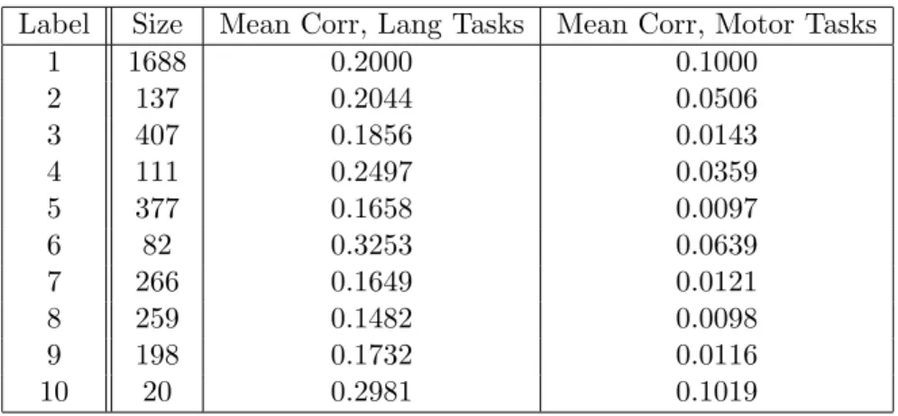
3.4 Summary of DC cliques found in Human Connectome Data . . . 51
4.1 Selected coherent word sets in Shakespearean tragedies . . . 83
4.2 Selected word sets in Shakespearean tragedies clustered by TF-IDF adjusted distance . . . 83
4.3 Coherent neighborhood for “Hannah Montana” . . . 86
4.4 Coherent neighborhood for “Paul McCartney” . . . 86
B.1 Gene lists for TCGA data . . . 102
C.1 Coherent word sets in Shakespearean tragedies . . . 104
C.2 Word sets in Shakespearean tragedies clustered by TF-IDF adjusted distance . . . 105
D.1 Coherent neighborhood for “Slayer” . . . 106
D.2 Coherent neighborhood for “Brandy” . . . 106
LIST OF FIGURES
1.1 Sample correlation matrices for each of two breast cancer tumor subtypes,
showing observed DC clique (A) and random genes (B) . . . 9
1.2 Ranks of genes in observed DC clique (A) out of 15,785 total genes. . . 9
3.1 Sample correlation of simulated data. . . 35
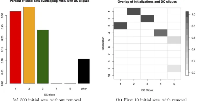
3.2 Overlap between initialized sets and DC cliques. . . 36
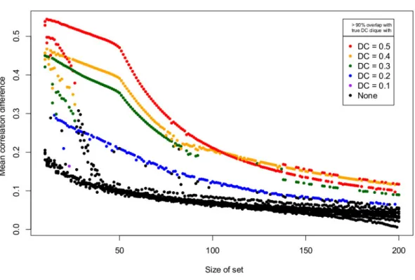
3.3 Initial sets at various sizes, colored by overlap with true DC cliques . . . 37
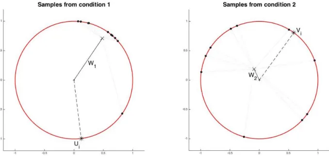
3.4 Geometric representation of data in two dimensions. . . 41
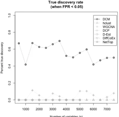
3.5 True discovery rates when false positive controlled at 0.05 level. . . 45
3.6 Sizes of incorrect variables sets when no differential correlation is present. . . 45
3.7 Detection rate for various dimensions. . . 46
3.8 Computation time to find a single variable set. . . 48
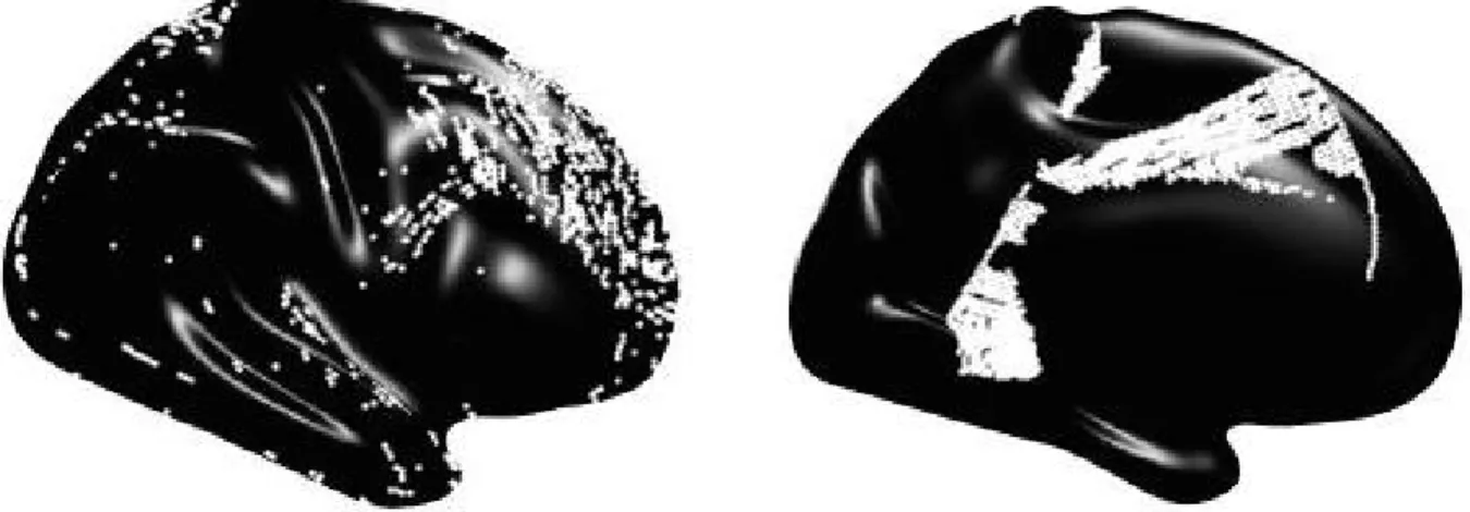
3.9 Brain locations of DC clique for languages tasks versus motor tasks. . . 52
3.10 Brain locations showing high first-order differences and high non-differential correlation. . . 52
4.1 Toy Dataset . . . 59
4.2 Hierarchical clustering dendrogram for toy dataset. . . 61
4.3 Association matrices based on correlation and coherence for toy dataset. . . 62
4.4 True discovery rate (when false positive rate<0.05) by signal latent correlation strength. 79 4.5 True discovery rate (when false positive rate < 0.05) at ρ = 0.6 by rate of exponential distribution onτ. . . 80
4.6 Number of incorrect variables selected, by signal latent correlation strength. . . 81
LIST OF ABBREVIATIONS AND SYMBOLS VSAT DCM CSM FPR TDR TCGA d n
[d],[n]
A
m
ζ(j, A)
S(j, A) p(j, A)
A(X, α) X
˜ X
R1,Rˆ1
ρjk, rjk
∆(j, A) Ω P0(·)
φ(·)
ϕ(·)
L(· | ·) I{·}
Variable-to-Set Testing
Differential Correlation Mining Coherent Set Mining
False Positive Rate True Discovery Rate The Cancer Genome Atlas
The dimension of data, i.e., the number of variables of interest The sample size, i.e., the number of d-dimensional observations The set of indices {1, . . . , d} or{1, . . . , n}
A variable set A⊂[d]
The size of a variable set, |A|=m
A population association measure between variable j and set A
A statistic for testing ζ(j, A)>0
The p-value pertaining to a test of association between j and A
The set of VSAT fixed points at level α for dataX An observed data matrix of dimension n×d
An appropriately standardized version ofX
The d×dpopulation and sample correlation matrices for dataX1 The population and sample correlations between variables j and k
The average correlation difference between j and A
An n×dmatrix of realizations of random parameters The probability under a suitable null measure
The standard Normal cdf The Fisher transformation
CHAPTER 1
Introduction
The field of statistics first developed as a way of drawing conclusions from limited observations. Today, statisticians face a nearly opposite challenge: how to glean meaningful information from an ever-growing supply of data. The term “data mining”, once a controversial epithet for questionable practices, now refers optimistically to the practice of extracting valuable material that has been buried in debris. In general, data mining methods seek notable patterns among noisy observations. Many such methods are exploratory, in that they focus on discovery rather than verification. Sta-tistical data mining, more specifically, makes use of modeling and testing principles both to identify patterns and to make probabilistic claims about their validity. As available data becomes higher dimensional and more complex, approaches to problems of statistical data mining must continue to adapt in response.
This dissertation introduces novel statistical methods for the branch of data mining known as association mining. In general, association mining is concerned with detecting relational (or second-order) structure between variables. For example, a company might study association between its employees, with the goal of identifying distinct social subgroups or of understanding how low-level employees interact with management. Association structures of interest vary by data type and by research question. Most commonly, association mining targets take the form of subsets of variables that are either strongly internally associated or all associated with a common external feature. The work in this dissertation is specifically concerned with the former.
1. Distance or dissimilarity.
Often, information about variables can be summarized in a single dissimilarity matrix, where entries represent pairwise relationships. In some cases, these matrices are calculated from data. For instance, if variables represent points in a vector space, the relationship between two points can be represented by a distance metric. In other cases, dissimilarity matrices are observed directly rather than computed. Such is the case in the analysis of networks, where available data takes the form of a set of variables (or nodes) and a set of links (edges) between the nodes. Edges may be weighted, taking on continuous values, or unweighted, consisting of 0/1 indicators of presence or absence. The measure of association between two variables is therefore the value (or presence) of the edge between those variables. In general, association mining based on dissimilarity measures or on network data is not statistical, in that the measures of association are treated as non-random. However, ran-domness can be introduced via addition of noise to dissimilarity measures or assumption of generating models. A prominent example of this is the Erdos-Renyi random graph model (Robins et al., 2007), which assumes an observed unweighted network was created by ran-domized edge assignments.
2. Estimators for statistical dependence.
When data can reasonably be considered random samples from a population, it makes sense to infer relationships via estimates of parameters. Perhaps the most commonly studied parameter is the standard product-moment correlation,
cor(X, Y) := EpXY −EXEY
var(X) var(Y)
The advantage of mining for association in the form of correlation is that two variables with nonzero correlation necessarily have nonzero dependence, and thus a “true” relationship may be said to exist. There are many alternatives to product-moment correlation, including partial correlation, rank-based correlation and covariance. It also should be noted that estimators
ˆ
One limitation of the correlation and related dependence measures is that they capture only linear relationships between variables. More complex dependence can be represented by summary statistics of graphical models, see e.g. Anderson (1959) Chapter 9 for further detail. Recent work has also produced useful estimators of nonlinear dependence, notably: Sz´ekely et al. (2007) defines thedistance correlation, which is equal 0 for a variable pair if and only if the variables are independent; and Zhang (2017) proposes a distribution-free procedure for detecting dependence. Tan et al. (2002) provides a thorough overview of the many other available measures of dependence.
The methods in this dissertation are strictly statistical, and so content will primarily focus on association mining in the context of estimators for statistical dependence. Section 1.4.2 provides a more in-depth discussion of the consequences of different measures of association, as a motivation for the new measure (and corresponding mining methodology) introduced in Chapter 4.
1.1 Contributions and Outline
This dissertation consists of an in-depth treatment of two new methods for association mining: Differential Correlation Mining (DCM) and Coherent Set Mining (CSM). Differential Correlation Mining is an algorithm for discovering variable sets that exhibit different correlation structure across two predefined sample conditions. Coherent Set Mining offers a method for mining for latent association structure from binary thresholded observations. Both methods are built on a novel algorithmic framework for mining strongly associated variable sets (or “communities”), known as Variable to Set Affinity Testing (VSAT).
1.2 Background: methods of association mining
Existing work in data mining can be characterized as either unsupervised orsupervised. Unsu-pervised learning consists of searching for patterns in data without regard to a predictive goal. In supervised studies, datasets consist of a limited number observations for which a ground truth is known, from which one usually makes inferences about future behavior. For example, simple linear regression infers the nature of a linear relationship between a measurementx and random variable
Y from observed pairs (xi, yi)ni=1. Data mining tasks can also besemi-supervised, in that a ground truth is known about only some of the available observations. This “training data” is then used to infer information about the remaining (or future) observations.
Perhaps the most well known class of unsupervised association mining methods is clustering algorithms. Clustering is the practice of dividing variables into groups, orclusters, that are highly internally associated. Typically, clustering methods seek a partition of the variables, such that each variable is assigned to exactly one cluster. In some settings, finding a partition of data is not appropriate to the research question at hand. For example, consider the problem of identifying social group memberships based on an observed Facebook friendship network. A strict partition of individuals does not capture the desired structure, since people may belong to many social groups or even none at all. Clustering tasks on networks are often referred to as community detection (cf. Fortunato (2010); Newman (2006) among others).
Although the methods of this dissertation are unsupervised, association mining also plays a role in some supervised and semi-supervised approaches. Most notable are classification and ma-trix completion problems. Classification refers to analyses of data for which there exist pre-specified categories. Typically, category labels are known for a given subset of observations, and new observa-tions are assigned to categories based on their association with known members. Matrix completion, by contrast, usually assumes one has incomplete observations for a number of variables. One then “completes” the matrix by filling in missing values with estimates derived from similar variables. Chapter 5.3 discusses the use of association mining in matrix completion problems and suggests a future direction for improvement on these algorithms.
clustering, which will provide a standard basis of comparison for the new methods discussed in this thesis, as well as for an area of supervised association mining that has a close relationship to the methods in this dissertation.
• k-means clustering.
The k-means clustering algorithm consists of a simple iterative update to minimize an objective. The algorithm begins with a randomly chosen k data observations, designated as “centroids”. The remaining observations are then assigned membership in one of the k
clusters characterized by the centroids, in such a way as to minimize the total sum of squared error for the partition. The centroids are then updated to be the geometric centers of each of these clusters, and the process is repeated until convergence. The k-means method is similar to the common K-nearest neighbors approach, in that both cluster objects around a centroid. However, K-nearest neighbors analyses do not produce a partition, but rather study individual target objects via theK closest objects.
There are two main reasons for the ubiquity of thek-means method. First, it is extremely computationally efficient, and can be run quickly and without large memory demands even for very high dimensional data. Second, it has a close tie todimension reduction techniques. When a dataset consists of observations in d dimensions, it is common to use Principal Component Analysis (PCA) to reduce the dimension before applyingk-means. The practice of dimension reduction before clustering includes a class of methods known asspectral clustering. PCA and k-means share a unique relationship even among spectral clustering methods due to a theoretical link between clusters centers and dimensions (Ding and He, 2004).
• Hierarchical clustering.
or splitting variable sets. For example, Section 4.5.1 compares the results of hierarchical clustering for a variety of choices of linkage metrics.
The output objects of a hierarchical clustering algorithm are dendrograms indicating at what height, or value of the linkage criteria, variable sets were divided/merged. To select a particular partition of the data, one typically determines a cutoff height of the dendrogram. When hierarchical clustering appears in this thesis, as a basis for comparison in simulation studies, we circumvent this problem by comparing our methods only to the best possible choice of cutoff as determined by “oracle” information about the true nature of simulated data. However, in practice, the decision about where to cut a dendrogram has enormous influence on the results. Contributions to the field of hierarchical clustering generally involve suggested algorithms for cutting a dendrogram for a particular data setting and linkage criteria.
• Variable selection by penalized regression.
As a rule, data mining is descriptive rather than predictive; that is, its primary purpose is to use observations to identify structure in variables, rather than to forecast future observations. Regression analysis, on the other hand, is commonly used for prediction. Recent work has adapted regression principles to methods of variable selection. Perhaps the most notable examples are the penalized regression techniques of Tibshirani (1996) and Zou and Hastie (2005), which use an L1 and L2 penalty (respectively) to forcibly reduce the number of explanatory variables incorporated in the model. In many applications, researchers are more interested in which covariates are selected for inclusion rather than the predictive power of the model. For instance, in statistical genetics, one may use penalized regression to determine which genes among thousands are most correlated with a particular phenotypic response.
1.3 Differential Correlation Mining
In many statistical problems, one has two datasets that measure the same variables under different conditions. It is common in the analysis of such data to assume that the samples in each dataset are generated from two underlying distributions. Even when the data is high dimensional, differences between the distributions may be present for only a small number of variables, and it is often of interest to identify these key variables. Most often, differential behavior between sample groups is measured by first-order statistics, which are functions of a single variable. Familiar first-order statistics include the sample mean and the sample variance. A well-studied example of first-order differential analysis is the study of differential gene expression in microarrays (see Cui and Churchill (2003) for a canonical example, or Soneson and Delorenzi (2013) and the references therein for an overview of several methods). Other applications of first-order differential analysis include text analysis for authorship identification (Stamatatos, 2009), studies of brain functionality based on regional activation (Phan et al., 2002), and investigation of cultural bias in standardized testing (Wainer and Braun, 2013).
The use of first-order statistics allows for analysis of only a single variable at a time. To study relationships between pairs of variables, one requires a measure of association such as correlation. Kriegel et al. (2009) provides a survey of clustering methods for high-dimensional data based on correlation distance. Datta and Datta (2002) and Jiang et al. (2004) and the references therein give an overview of methods developed specifically for clustering of gene expression. In general, typical clustering or community detection methods must be adapted for application to correlation distances to correct for bias (see e.g. MacMahon and Garlaschelli (2015) for an illustrative example). In applications of non-differential correlation mining, variable groups may represent, e.g., social groups communication networks (Lewis et al., 2008), genes in common protein pathways (Jiang et al., 2004), or functionally similar brain regions (Greicius et al., 2002).
one studies two different sets of variable relationships. In some cases, simply taking the difference of dissimilarity matrices and applying ordinary clustering methods would suffice. However, most second-order statistics - including the linear correlation coefficient - require a more careful treat-ment. For instance, two sample correlation matrices will exhibit vastly different random behavior based on the sample sizes of the corresponding datasets, and will have a complex dependency structure when the corresponding population correlation matrices are not the identity.
Chapter 3 introduces Differential Correlation Mining (DCM), a new method of second order comparative analysis that identifies sets of variables such that the average pairwise correlation between variables in the set is higher in one sample condition than in another. The method does not make use of auxiliary information, apart from the separation of samples into pre-determined groups (e.g. treatment vs control). Differential Correlation Mining is theoretically applicable to both low and high dimensional settings and is computationally feasible for high dimentional data (105 variables).
1.3.1 Example: TCGA
The following real-world example provides a brief illustration of and motivation for Differential Correlation Mining . Figure 1.1 shows a differentially correlated variable set identified by the DCM procedure in real data from The Cancer Genome Atlas (TCGA) Research Network (http: //cancergenome.nih.gov/). The two sample conditions under consideration are Her-2 type breast cancer tumors and Luminal B type tumors, as classified by (Perou et al., 2000). Further results for the TCGA dataset are provided in Section 3.7.
Figure 1.1: Sample correlation matrices for each of two breast cancer tumor subtypes, showing observed DC clique (A) and random genes (B) .
In general, the results of Differential Correlation Mining are distinct from those found by first-order analysis (e.g. differential expression). For example, Figure 1.2 shows the relative differential expression, overall expression level, and differential variation for the above estimated DC cliqueA. In this plot, all genes in the study (p =15,785) are ranked by (a) t statistic of differential mean expression between Her-2 and Luminal B samples, (b) overall expression in Her-2 samples, and (c) ratio of sample variations (F statistic) for Her-2 versus Luminal B samples. The histograms in Figure 1.2 show the ranking of the genes inA. The overall uniformity of the histograms indicates that the variables in the observed DC clique A do not exhibit standard first-order differential behavior.
Figure 1.2: Ranks of genes in observed DC clique (A) out of 15,785 total genes.
(Ranked by: Differential expression, as measured by p-values of 2-sample t-tests; mean overall expression among
By targeting differentially correlated variable sets, the Differential Correlation Mining method identifies variables whose joint behavior is different across sample conditions. The results are readily interpretable as sets of variables that interact strongly under one sample condition but only weakly (or not at all) under another.
1.3.2 Related work
Much existing work is either directly related to differential association or may be reasonably adapted to such a paradigm. In what follows, letR1,R2denote the population correlation matrices of two data distributions, and let Rb1,Rb2 denote the corresponding sample correlation matrices.
1. Mining from single correlation matrices.
Non-differential correlation mining has been well-studied, typically in the context of clus-tering. These methods may be applied in the differential case by separately clustering the correlation matricesRb1,Rb2 and comparing results.
2. Detection of isolated changes in correlation structure.
Existing approaches to differential correlation mining are largely based on examining in-dividual variables for changes in second-order structure across two sample conditions. For example, one may treatRb1 andRb2as the adjacency matrices of two fully connected, weighted
networks, and then look for variables whose connectivity pattern is very different across the two networks (Xia et al., 2014; Gill et al., 2010). Most methods approach differential corre-lation mining by developing a statistic to measure the change in pairwise correcorre-lations of an individual variable: Hu et al. (2010) uses the covariance distance (total difference of covari-ances), Choi and Kendziorski (2009) uses a direct difference of sample correlations, Fukushima (2013) uses the difference of Fisher transformed sample correlations, and Liu et al. (2010) use a filtration (or thresholding) step before summing square correlation differences. These meth-ods then permute samples across the two classes to measure the significance of the original differential correlation. Significant variables may then be selected by an appropriate multiple testing procedure.
There has been a great deal of theoretical work devoted to testing equality of high-dimensional covariance and correlation matrices. When the sample size n is substantially larger than the dimension p, classical results are applicable, e.g., likelihood ratio tests as discussed in Anderson (1958) and Muirhead (1982), or results like those of Steiger (1980) for testing individual sample correlation. In the high-dimensional (p > n) setting, Cai et al. (2010), Cai and Jiang (2011), and Cai et al. (2014) have developed minimax rate optimal tests for the equality of covariance matrices under sparsity assumptions. Results for correlation (rather than covariance) are less prevalent; recent work includes tests for sets of sample cor-relation coefficients (Donner and Zou, 2014), tests for rank-based corcor-relation matrices (Zhou et al., 2015), and tests for detecting overall dependence (Bassi and Hero, 2012).
In some cases, optimal testing procedures can inform methods for estimation of high-dimensional covariance and correlation matrices. Particularly relevant is the work of Cai and Zhang (2014), which yields an estimator for the difference matrix D = R1−R2. This estimator is implemented and discussed further in Section 3.6. Other approaches to high-dimensional estimation include: Bickel and Levina (2008), who discuss a thresholding esti-mator for covariance matrices; Peng et al. (2008), who estimate partial correlations in sparse regression models; and Rajaratnam et al. (2008), who make use of graphical model techniques for covariance matrix estimation.
4. Direct mining of differential correlation
1.4 Association Mining in Binary Data
The majority of well-known association mining methods are implicitly designed for continuous data. However, in some common settings, data may take the form of binary (0/1) observations. For example, purchasing information - known asmarket basket data - often consists of observations about ditems available for purchase by nbuyers. The resulting data matrixX∈ {0,1}n×d, where
Xij indicated whether buyer i bought item j, therefore may be interpreted as n samples of a d -dimensional binary random variable. It may be of interest to identify association structure in these
dvariables from the nsamples.
In its basic form, this problem is not distinct from ordinary clustering and community detection methods. Algorithms like hierarchical clustering may be applied to any dissimilarity matrix, so as long as an appropriate measure of association is chosen, these methods still apply. However, binary data presents a unique challenge when it comes to standardization. Consider standardizing a vector in{0,1}n such that the sample mean is 0 and the sample variance is 1. The values{0,1} are then each transformed to a different pair of values. No real transformation has been applied to the data; it is still dichotomous. Measurements such as product-moment correlation, which rely on a standardization step, are therefore not as appropriate as metrics for associations studies.
A further challenge arises when samples are not treated identically. Measures of association that involve an unweighted average over sample quantities, such as L1 and L2 distances, are unequipped to account for different behavior between buyers. In continuous data, differences between samples are often swept under the rug via pre-processing of data, usually by sample-standardizing before variable-standardizing. This option is less appealing in the binary case.
The method introduced in Chapter 4, Coherent Set Mining (CSM), was developed to be flexible to sample heterogeneity without disregarding the inherent dichotomous nature of binary observa-tions. The following simple application motivates the need for such an approach, and give an overview of existing work in association mining that is specific to binary data.
1.4.1 Example: Grocery Store Data
grocery store transactions,Groceries, intended as ideal data for exploring and testing association mining methods. This dataset consists of observed 9835 transactions for 169 items. Tables 1.1 and 1.2 show the results of applying the well-knowneclatalgorithm and our new method, Coherent Set Mining, to the grocery store data. Since eclat screens for itemsets with support above a certain threshold, we applied the method with many thresholds. Table 1.1 shows the results for a threshold that yielded a moderate number of reasonably-sized itemsets. The Coherent Set Mining method, by contrast, is fully automatic and so the contents Table 1.2 are simply the direct output of the method.
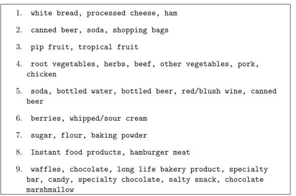
The results in Table 1.1 lack an obvious interpertation. All three frequent sets contain whole milk, the most common item in the Groceries dataset. Intuitively, this makes sense, because the eclatalgorithm seeks itemsets that appear in a large percentage of transactions; thus, items which are puchased more often overall are more likely to appear in frequent sets. The itemsets in Table 1.2, on the other hand, are readily interpretable in terms of real world grocery needs. For instance, Set 1 in Table 1.2 is easily recognizeable as a ham and cheese sandwich, Set 5 contains drinks one might buy for a party, and Set 7 evidently corresponds to baking staples.
Table 1.1: Results fromeclat with support threshold = 0.05
1. whole milk, other vegetables 2. whole milk, rolls/buns
3. whole milk, yogurt
This example is provided to briefly justify the need for a new approach to association mining in binary data. Chapter 4 offers an in-depth discussion of settings where existing methods are susceptible may be measuring association that is not of scientific interest. The Coherent Set Mining approach is designed with such settings in mind, to work around challenges like the overall frequency of whole milk and produce more meaningful results such as those in Table 1.2.
1.4.2 Related Work
Table 1.2: Results from CSM
1. white bread, processed cheese, ham 2. canned beer, soda, shopping bags 3. pip fruit, tropical fruit
4. root vegetables, herbs, beef, other vegetables, pork, chicken
5. soda, bottled water, bottled beer, red/blush wine, canned beer
6. berries, whipped/sour cream 7. sugar, flour, baking powder
8. Instant food products, hamburger meat
9. waffles, chocolate, long life bakery product, specialty bar, candy, specialty chocolate, salty snack, chocolate marshmallow
In principle, existing methods for clustering or community detection can easily be applied to binary data; one need only specifiy a measure of dissimilarity. However, there are many options for how best to infer relationships between variables from binary observations. (Choi et al., 2010) provide an overview of 76 different suggested dissimilarity measures (some of which are mathematically equivalent). Notable among these are the Phi Coefficient, which is equal to product-moment correlation, and the Jaccard distance, which considers a ratio of co-occurance to individual occurance. Some prior work also addresses the case of binary observations directly. Li and Li (2005) provide a general framework and methodology for clustering binary data, and Neuhaus et al. (1991) summarizes classic methods for analyzing correlated binary data.
• Frequent itemset mining and association rules.
inven-tory control, and so forth. Methods for mining in market basket data fall under the heading of frequent itemset mining or association rules. In general, approaches to frequent itemset mining are non-stochastic; instead of modeling the data, they proceed by screening datasets for sets of items whose support or percentage of buyers who purchased the entire itemset -is above a certain threshold. For example, a frequent itemset d-iscovered from grocery store purchases might take the form{milk, eggs, bread}.
The study of frequent itemsets and association rules arguably began with the work of Agrawal et al. (1996), which introduced theapriori algorithm. This method is built on the apriori principle: that for an itemset to be frequent, all of its subsets must also be frequent. The apriori approach vastly reduces the number of itemsets that must be screened to search a dataset exhaustively. Subsequent methods improved onaprioriby both algorithmic solutions and computational improvements. Some notable examples includeeclat(Zaki et al., 1997a), MAFIA (Burdick et al., 2001), COBBLER (Pan et al., 2004), fp-close Grahne and Zhu (2003), and CHARM (Zaki and Hsiao, 2002). Zaki et al. (1997b), Prabha et al. (2013), (Zaki et al., 1999) and the references therein provide an excellent summary of early and recent work in frequent itemset mining. There are also some exceptions to the non-stochastic nature of itemset mining. Zhang et al. (2008) estimates the probability of itemsets exceeding a specified frequency, rather than simply screening for itemsets exceeding a threshold. Aggarwal et al. (2009) and Tong et al. (2012) take more complex model-based approaches to data uncertainty. Instead of screening for high support, they screen for highexpectedsupport under a probability model.
CHAPTER 2
Variable-to-Set Affinity Testing
2.1 Introduction
In general terms, the goal of the association mining algorithms in this dissertation is to identify subsets of variables that are more associated internally than externally. Classical approaches to problems of this type typically rely on an optimization algorithm. That is, every variable set or every partition is given a score intended to measure the strength of in-group versus out-group association. For example, ink-means clustering (MacQueen, 1967), a particular partition is scored by the within-cluster sum of squared distances to means. These methods then apply a maximization (or minimization) procedure with the goal of identifying clusters or communities with high (or low) scores.
There three main challenges inherent to such approaches. First, if one has a moderate to large number of variables, it is in most cases computationally intractable to find global optima for a score. Instead, methods most commonly apply algorithms guaranteed to reach local optima, then run these localized procedures many times and select the “best” output. For instance, thek-means algorithm consists of a greedy iterative procedure to refinekcluster centers until the within sum-of-squares distance to center is locally minimized. Since the locally minimal choice of cluster centers may be different depending on the starting point, it is common to applyk-means multiple times to a particular dataset and report only the most optimal partition.
and Lancichinetti et al. (2011) imposes a model on networks and then measures significance of communities based on asymptotic extreme value results. It is also sometimes possible to derive measure of significance via a bootstrapping or permutation-based approach, see e.g. Jakobsson and Rosenberg (2007). However, these solutions all represent ex post facto assessments of clusters or communities; statistical principles are not embedded in the search algorithm itself.
Finally, existing methods of clustering and community detection commonly require crucial user input. In k-means and many other clustering methods, one must pre-select k, the number of clusters. In hierarchical clustering, the final selected partition depends on the choice of where to cut the dendrogram. For community extraction methods, it is usually necessary to specify a score threshold above which a community is considered “interesting”. Reliance on user-specified information weakens the conclusions of association mining as compared to a fully data-driven method.
As a response to some of the limitations of existing association mining techniques, the methods in this dissertation make use of the Variable-to-Set Testing (VSAT) algorithmic framework first introduced by Wilson et al. (2014). VSAT is a general approach to statistical association mining based in hypothesis testing principles. Methods built from the VSAT algorithm enjoy many advantages over classical clustering and community detection, such as flexibility to unusual data types and/or particular measures of association. Associated variable sets selected by VSAT algorithms have natural statistical interpretations and error control guarantees. Because VSAT type methods choose variable sets adaptively from significance testing results, one need not pre-specify a number or size of clusters or a score cutoff. Finally, implementations of VSAT algorithms tend in general to be computationally efficient. Importantly, the VSAT approach is not an optimization procedure. No score is involved; rather, sets are chosen organically via testing-based iterative update.
2.2 The variable-to-set testing algorithm
The VSAT algorithm relies on the determination of a population quantity of interest, a test statistic, and a null model. The choice of measure of association and assumptions about data for a particular analysis dictate the appropriate test statistic and null. This chapter provides a discussion of the VSAT framework in terms of a general choice of measure of association.
Formally, defineζ(j, A) to be a measure ofaffinity between variablejand variable set A⊂[d]. In general,ζ(j, A) is a function of the set of pairwise associationsa(j, k) betweenjand {k:k∈A}
for some choice of association measurea(·,·). Most VSAT methods will defineζ(j, A) to be a simple average overk∈A, that is,ζ(j, A) :=|A|-1P
k∈Aa(j, k). For example, to mine for highly correlated variable sets, one might seta(j, k) to be the population correlation ρjk between variablesj andk, then let ζ(j, A) be the average of these correlations. In general, however, ζ(j, A) may be chosen to reflect the association structure of interest in a particular research problem. Given a choice of
ζ(j, A), the VSAT algorithm is designed to use statistical principles to search for ζ-connected sets, defined as follows.
Definition 1. (ζ-connected set) An index set A⊂[d]with at least two elements is ζ-connected with regard to an affinity measure ζ(·,·) if
(i) for all j∈A, ζ(j, A)>0, and (ii) for allj /∈A, ζ(j, A)≤0.
A ζ-connected set may be thought of as “closed”, in the sense that only elements in the set have positive affinity (as measured byζ) with the rest of the set. The VSAT search procedure for
ζ-connected sets is summarized as follows.
1. Initialization: SetA0⊂[d].
2. Testing: GivenAt, simultaneously test hypotheses for the affinity of j∈[d] toAt,
by an appropriate multiple testing procedure. 3. Update: SetAt+1={j : H0(j) was rejected }.
4. Iteration: Repeat steps 3 and 4 untilAt=At0 :=A∗.
5. Output: IfA∗ is not empty, select it as an estimatedζ-connected variable set.
6. Repetition: Repeat steps 2-5 as many times as desired, or until no further sets are found.
Steps 2-5 may be considered a refinement process, during which a proposed ζ-connected setAt is updated in accordance with the results of simultaneous hypothesis tests. Regardless of the size of initial setA0, the size of output setsA∗ is chosen adaptively by the application of multiple testing. Furthermore, because updates require statistical significance, not every initial setA0 is guaranteed to produce convergence to a non-empty set A∗.
If t0 = t− 1, the sets A∗ are fixed points of convergence of the VSAT algorithm in that further updates will not change the elements of A∗. When t0 6=t−1, the algorithm has reached a cycle of three or more sets At, . . . , At0 that will continue ad infimum as the algorithm continues.
Although these sets are not as ideal as fixed points, which are discussed below, they are often highly overlapping and may be of interest. Particular implementations of VSAT methods take different approaches to cycles. For the remainder of this chapter, we restrict our discussion only to fixed points, or stable sets, which have several desirable properties.
Definition 2. (Stable Set) Let Uα(A,X) denote the index set of the rejected hypothesis tests for
ζ(j, A) = 0 from observed data X. An index setA∗ ⊂[d] is a stable set in X if Uα(A∗,X) =A∗. Note, trivially, that A∗ =∅ is always stable set, albeit not one of scientific interest. There is a close relationship between nonempty stable sets and theζ-connected variable sets they approximate. A stable set A∗ has the property that for hypothesis tests H0(j) : ζ(j, A) = 0 performed on a particular observed dataset,
(ii) for allj /∈A,H0(j) was accepted.
It is clear thatA∗ exhibits the properties of Definition 1 up to a level of statistical significance. As such, the VSAT algorithm is a natural approach to estimating ζ-connected sets from data X.
2.3 Deriving hypothesis tests
The crucial element of the VSAT algorithmic framework is the ability to test the hypotheses in (2.1) for a desired affinity measureζ. In order to develop a VSAT type method for a particular association mining setting, one requires
1. A random vector or matrixX, containing information about variables 1, . . . , d
2. A test statistic S(j, A|X) for ζ(j, A) ; and
3. A null model P0 specifying the distribution ofS(j, A|X) whenζ(j, A) = 0.
The test statistic S(j, A|X) will in most cases be a direct estimator forζ(j, A) from X, such that large positive values provide evidence forζ(j, A)>0. Then, p-values pertaining to the hypotheses in (2.1) can be computed from an observed datasetXby
p(j, A|X) :=P0(S(j, A|X)> S(j, A|X)). (2.2)
In other words, the p-values measure the extremity of the observed dataXunder the a null distri-bution on X.
In other settings, X may simply represent a single instance of a dissimilarity matrix. Such is the case in the existing VSAT methods for networks (Wilson et al. (2014), Palowitch et al. (2016)). Observed data in these cases takes the form of a network or a series of networks, represented by a node set [d] and a (possibly weighted) edge set E capturing relationships between nodes. To perform inference on these artifacts, a specific null generative model is assumed appropriate to the data context. Then, the distribution P0 on S(j, A|X) can be derived from this null model.
Remark: Ancillary Statistics. Commonly, the null measureP0, or asymptotic approxima-tion thereof, will depend on an unknown parameter η that has no bearing on the measure ζ of interest, but that nonetheless must be estimated from data. For instance, in the example of basic correlation mining, the asymptotic distribution supplied by Steiger and Hakstian (1982) depends in part on the covariance between sample correlations, for which an explicit form is derived in terms of the population moments. In practice, one must estimate the covariances from sample estimates of moments in order to compute p-values. Ideally asymptotic results regardingP0 continue to hold when η is replaced by a data-driven estimate ˆη.
2.4 Flexibility in objective
An association mining method by the VSAT approach is fully specified by a choice ofS(j, A|X estimating ζ(j, A) and a null model P0. Therefore, in principle, one can use this framework to perform association mining for any data feature of scientific interest that can be reasonably rep-resented as a ζ-connected set for some ζ. Notions of pairwise variable relationships that do not lend themselves well to the creation of a single summarizing dissimilarity matrix, necessary for most association mining methods, are still possible to study under via VSAT algorithm. The two methods derived in this thesis, Differential Correlation Mining and Coherent Set Mining, take full advantage of the flexibility inherent to the VSAT algorithm.
2.4.1 VSAT and Differential Correlation Mining
terms of the VSAT framework,
ζ(j, A) = 1
|A| X
k∈A
(R1−R2)jk and S(j, A|X) = 1
|A| X
k∈A
b
R1−Rb2
jk , (2.3)
where R1,R2 are population correlation matrices under two sample conditions and Rb1,Rb2 are
the usual sample correlation matrices computed from observed datasets of samples from the two conditions, X1 and X2. In the Differential Correlation Mining method, P0 is approximated by a Gaussian measure based on a central limit theorem for S.
The VSAT flexibility comes into play with regard to the covariance matrix of the test statistic,
{cov (S(j, A), S(k, A))}j,k∈A, which is needed to approximate P0. If one were to apply ordinary clustering or community detection to the adjacency matrixRb1−Rb2
, one would not be account-ing for variability in average correlations of a set A. The Differential Correlation Mining method allows us to estimate the necessary covariance from data, and therefore to testζ(j, A) directly. Es-timated ζ-connected sets are then interpretable as variable sets that have higher average pairwise correlation in the first sample condition, up to a level of statistical significance.
2.4.2 VSAT and Coherent Set Mining
Section 1.4.2 introduced the challenges of association mining from binary observations, and gave an example of data for which existing methods are not appropriate. Our approach to this problem, described in detail in Chapter 4, is to model binary data as a thresholded version of unobserved latent data. The measure of association of interest is the correlation in thelatent data, i.e., a(j, k) = cor(Zj, Zk) for some latent variableZ∈Rd and ζ(j, A) is the average of correlations between Zj and {Zk}k∈A. However, only a thresholded version of Z given by X ∈ {0,1}d is observed. In this setting, one does not have enough information to directly estimate the correlation structure of Z. That is, it is not possible to craft a test statistic that is a reasonable estimator for
ζ(j, A).
for large values ofζ(j, A). Our null model P0 is then derived in part from a central limit theorem, and in part from imposed null assumptions about the thresholding of ZtoX.
Coherent Set Mining, in other words, is an association mining method capable of estimating
ζ-connected sets,even though ζ itself cannot be estimated. The power of the VSAT framework lies in its flexibility to uncommon choices of ζ driven by unique data, and to choices of P0 driven by specific research questions
2.5 Control of global familywise error under the null
Since VSAT algorithms incorporate a multiple testing step at each iteration of the set update process, it is reasonable to expect that error control properties hold for the entire procedure. Indeed, it can be shown that in an idealized setting for small α, the probability of false identification is controlled.
This result, while simple, is important: it guarantees that in data where no signal is present (as defined by P0), the probability of any stable set being present is controlled at level α. Inter-estingly, (2.4) is a familywise error control property, even though the multiple testing procedure of (Benjamini and Hochberg, 1995) only controls False Discovery Rate. Theorem 1 allows us to have confidence that stable sets discovered by a VSAT type algorithm are likely to reflect true population structure.
Theorem 1. (VSAT global error control)
Fix α ∈ (0,0.15]. Let A(X, α) be the class of all stable sets of a VSAT algorithm using the Benjamini-Hochberg multiple testing procedure (Benjamini and Hochberg, 1995) at levelα. Assume that for any A⊆[d], the p-values {p(j, A|X) :j ∈[d]} are independent and uniformly distributed. Then,
P0 |A(X, α)|>0
< α . (2.4)
where P0 denotes the probability under the null model for X.
2.5.1 Example
asymptotic uniformity of p-values can be guaranteed by deriving a limiting distribution on the test statistic. Independence, however, is not always a reasonable assumption. The following example provides a setting where both conditions of Theorem 1 are met.
Example 2.1. Let P ={pjk} ∈[0,1](d×d) be a matrix of fixed probabilities, with pjk not neces-sarily equal topkj. Define the measure of affinity for an index j and a setA⊂[d] to be
ζ(j, A) = 1
|A| X
k∈A
pjk− 1
d− |A| X
k∈AC
pjk. (2.5)
Let X ∈ {0,1}(d×d) be a random matrix with X
jk ∼ Bernoulli(pjk), all independently. Suppose i.i.d. copies X(1), . . . ,X(n) are observed. Define the test statistic for an indexj and a setA⊂[d] to be
S(j, A|X) = 1
n n X i=1 1
|A| X
k∈A
Xjk(i)− 1
d− |A| X
k∈AC Xjk(i)
. (2.6)
Finally, let the null model P0 be thatpj1 =. . .=pjd =pj for every j. Then, ζ(j, A) = 0 for allj
and for any A⊂[d]. ♦
The data in Example 2.1 can be interpreted as a set of i.i.d. samples of a directed unweighted network. For example, the data might represent observations of behavior over time for a group of individuals, withXjk(i) representing whether individual j visited the Facebook page of individual
kon dayi. Then, aζ-connected set under the definition of ζ(j, A) would be a group of individuals who visit each others pages on average more than they visit other people’s. The null model may be interpreted as an assumption that each individual visits all her friend’s pages equally often.
Since observations Xjk(i) are binary, S(j, A|X) is bounded in [1,−1]. Therefore, since
S(j, A|X) is a sum of bounded i.i.d. variables, an ordinary central limit theorem applies. Note that the mean of S(j, A|X) is 0 under the null model, and its variance is given by
var(S(j, A|X)) = 1
n
1
|A|2
X
k∈A
var(Xjk) + 1 (d− |A|)2
X
k∈AC
var(Xjk)
= 1 n 1
|A|+
1 (d− |A|)
It is straightforward to show that ˆ
pj := 1 nd n X i=1 X k∈[d]
Xjk (2.8)
is a consistent estimator for pj under the null. Then, ˆσ(j, A) := d n-1(d− |A|)-1(ˆpj(1−pˆj) is consistent for the variance ofS(j, A|X). Therefore, underP0, for fixed A, p-values given by
p(j, A|X) = 1−Φ
S(j, A|X) ˆ
σ(j, A)
, (2.9)
where Φ(·) is the standard normal cdf, are asymptotically uniformly distributed. Finally, due to the fact thatpjk 6=pkj and that the variablesXjk are independent, it follows thatS(j, A|X) and ˆpj are independent ofS(k, A|X) and ˆpk for anyj6=k. Then, p(j, A|X) and p(k, A|X) are independent for j 6=k. We conclude that the setting in Example 2.1 asymptotically satisfies the conditions of Theorem 1.
2.5.2 Proof
Define Cm :={A:|A|=m}. By construction of the Benjamini-Hochberg procedure, the event thatA∈ Cm is a fixed point only if
\
j∈A
n
p(j, A;X)≤ mα d
o \ \
j∈[d]\A
n
p(j, A|X)> mα d
o
(2.10)
Since the p-values are independent and uniformly distributed, this implies that for any A∈ Ck,
P0 uα(A) =A
=mα
d
m
1−mα d
d−m
(2.11)
DefineAm(X, α) to be the class of all stable sets of sizem. Then, using equation 2.11 and a union bound,
P0 |Am(X, α)|>0
≤ d m mα d m
1−mα d
d−m
(2.12)
Applying the inequality md ≤ √1
2π( ed m)
m gives
√
2π P0 |Am(X, α)|>0
≤(eα)m
1−mα d
d−m
Since A(X, α) =∪Am, a union bound gives
√
2π P0 |A(X, α)|>0
≤
d
X
m=2
(eα)m= d
X
m=1
(eα)m−(eα)
Asα≤0.15<1/e, the sum on the right-hand side is a geometric series. Thus,
√
2πP0 |A(X, α)|>0
≤ eα[1−(eα)
d]
1−eα −eα≤
(eα)2
1−eα (2.13)
We want to show thatP0 |A(X, α)|>0
≤α, i.e., that
(eα)2 1−eα ≤
√
2πα . (2.14)
CHAPTER 3
Differential Correlation Mining
3.1 Introduction
Given data obtained under two sampling conditions, it is often of interest to identify variables that behave differently in one condition than in the other. In this chapter, we present a method for differential association mining calledDifferential Correlation Mining (DCM). The Differential Correlation Mining method identifies differentially correlated sets of variables, with the property that the average pairwise correlation between variables in a set is higher under one sample condition than the other. Differential Correlation Mining is a VSAT-style algorithm, so updates are performed via hypothesis testing of individual variables, based on the asymptotic distribution of their average differential correlation.
We refer to the target variable sets of Differential Correlation Mining as differentially correlated (DC) cliques. In a graph, a clique is a set of nodes that is fully connected, in the sense that there is an edge between every pair of nodes in the set. Informally, a DC clique is a set of variables such that each variable in the set has a positive (usually large) average differential correlation with the other variables in the set. More formally, let R1,R2 be the d×dpopulation correlation matrices of the distributions underlying sampling conditions 1 and 2, respectively. Let A⊂[d], where [d] is the index set {1, ..., d}, and define
∆(j, A) = 1
|A| X
k∈A
(R1−R2)jk (3.1)
Definition 3. Let R1,R2 be given and let∆(·,·) be defined as in (3.1). An index set A⊆[d]with at least two elements is a DC clique for R1−R2 if
1. ∆(j, A)>0 if and only if j∈A,
2. The set A cannot be written as a disjoint union of nonempty index sets A1, A2 ⊂ [d] such thatA1 andA2 satisfy condition 1 above.
Condition 1 ensures that no relevant variables are omitted from a DC clique (every variable that is positively differentially correlated relative to the setAis included inA) and that a DC clique does not contain any extraneous elements. Condition 1 implies that a DC clique has larger average pairwise correlation under the first distribution than under the second. Condition 2 ensures that a DC clique cannot be subdivided into two smaller DC cliques. Importantly, the definition placesno conditions on the correlation matrices R1 and R2. In particular, R1 and R2 need not be sparse, and need not satisfy any structural constraints such as bandedness. For a given pair R1,R2, it may happen that no DC cliques exist, or that the entire variable set forms a DC clique.
Note that the definition of DC cliques is not symmetric: in general, the DC cliques forR1−R2 will be different from those for R2−R1. The difference lies not in the relational structure itself, but rather in how we order the sample conditions (1 or 2). For example, in biological data, one sample group may involve a treatment condition, while the other is a reference or control group. A DC clique forR1−R2 would contain genes that are more highly correlated in Condition 1 than Condition 2, for example, a protein pathway that is more active in Condition 1. This structure is illustrated in Figure 1.1.
The asymmetry in DC cliques could be eliminated by replacing the relevant section of (3.1) by a symmetric notion of difference such as |R1−R2|. However, a variable set based on absolute difference (or similar) could contain a mixture of elements with positive correlation to A and elements with negative correlation to A. Such mixed groups would not exhibit the unified block structure of the type seen in Figure 1.1. Further, large variable sets with strong average negative correlation cannot occur. Simple algebra shows that since R1 is positive definite, the average pairwise correlation in Condition 1 of any set A withm elements must be at least -(m−1)1 .
in these estimators, to select empirical DC cliques. The broad objective of Differential Correlation Mining is to use observed data to identify DC cliques, or approximations of these, without prior knowledge of the identity, number, or size of the DC cliques present in the population. It is worth noting that the Differential Correlation Mining algorithm and supporting analysis described here are easily adapted to a non-differential correlation mining algorithm. An implementation of a correlation mining procedure is included along with the public DCM software.
Notation. In what follows, we assume that the data under condition 1 consists ofn1independent samples drawn from a distributionF1with correlation matrixR1, and that the data under condition 2 consists ofn2 independent samples drawn from a distributionF2 with correlation matrixR2. Let X1 = (U1, ...,Ud) ∈ Rn1×d and X2 = (V1, ...,Vd) ∈ Rn2×d denote the resulting data matrices in standard sample-by-variable form. Thus Uj ∈ Rn1 denotes the measurements of variable j under condition 1, whileVj ∈Rn2 denotes the measurements of variable j under condition 2. Let X1,A = (Uj)j∈AandX2,A= (Vj)j∈Adenote the restriction ofX1 andX2, respectively, to a variable set A ⊂[d]. Similarly, let R1,A and R2,A denote the correlation matrices under the distributions of F1 and F2 restricted to the variables inA.
Let ˜Uj and ˜Vj be the standardized versions of Uj and Vj respectively, such that kU˜jk =
kV˜jk = 1, and define ˜X1 = ( ˜U1, ...,U˜d) and ˜X2 = ( ˜V1, ...,V˜d). Finally, let Rb1 and Rb2 denote
the usual sample correlation matrices of X1 and X2, respectively (and Rb1,A and Rb2,A those of the
appropriate restricted datasets). Thus Rb1
jk = cor (c Uj,Uk) = X˜
t 1X˜1
jk and a similar relation holds for Rb2.
3.2 The Differential Correlation Mining Method
An important advantage of this type of approach is that the number and size of output sets are chosen adaptively based on testing principles. The Differential Correlation Mining method does not require pre-specification of number of clusters (as in kmeans), nor does it require an additional decision about cluster size (as in hierarchical clustering). Rather, the multiple testing procedure in the iterative step of Differential Correlation Mining naturally determines the number of variables in an output set. Differential Correlation Mining also differs from typical clustering procedures in that it does not require the calculation of a fulld×ddissimilarity matrix, which can be a computational advantage in high dimensional data.
The Differential Correlation Mining procedure is summarized below. Detailed pseudocode is in Appendix A.
The Differential Correlation Mining Method
1. Initialization: Identify a good initial variable setAusing a greedy algorithm that identifies a local maximum of a simple score function.
2. Iteration: Refine the initial set A. At each iterative step, repeat the following until termination.
B Test the differential correlation of each variable j with respect to A. Let A0 be the set of variables with significant differential correlation, as determined by an FDR controlling multiple testing procedure.
B Terminate ifA0=Aor a cycle is observed. B Update: SetAto be A0.
3. Return: Output variable setA.
Iterative updating using multiple testing was first applied by Wilson et al. (2014) in the context of community detection for binary networks. Differential Correlation Mining makes use of the same search paradigm; however, a fundamentally different treatment is required to address differential correlation. In particular, the work of Wilson et al. (2014) performs hypothesis tests based on a fully constructed null model, whereas Differential Correlation Mining requires no structural assumptions on the null distribution of the data beyond equal correlation (R1 =R2) and some mild moment conditions (see Theorem 2).
3.2.1 Minor Algorithmic Details
Residualization In general, we expect multiple DC cliques in a dataset. The residualization step allows the Differential Correlation Mining procedure to search the same dataset many times, avoiding repeated results. Suppose an empirical DC clique A has been selected. Our approach is to estimate a rank one approximation of correlation matrices Rb1,A and Rb2,A via factor analysis
(Harman, 1960). We then substitute the relevant submatrices, X1,A and X2,A, with residualized data for which the estimated rank one correlation has been removed. Methods of estimation and removal of low-rank correlation have been well established in the literature. In the DCM software, we use the implementation of Friguet et al. (2012) for the R Statistical Software version and the method of Bishop (2006) for the Matlab version.
By opting for rank-one approximation, we are taking a conservative approach to residualization. It is conceivable that the correlation structure ofAis of higher rank. If so,Amay be selected more than once; however, since each time the data is being further residualized, we are guaranteed to eventually remove all structure ofA. In practice, we have yet to encounter a duplicate result from real data.
disjoint DC cliques. Further runs of the Differential Correlation Mining algorithm are then able to identify the separate DC cliques.
In extreme cases, the sampled data may be such that the disjoint DC cliques are, by chance, correlated enough to have negligible remaining individual structure after residualization. This correlation may render the multiple DC cliques indistinguishable in the data from a combined DC clique.
Cycles. Under certain conditions, the main search procedure terminates in a cycle of two or more sets. When the set update procedure oscillates between two sets A1 and A2, we restart the search on the intersectionA=A1∩A2. In this case, the algorithm usually converges to fixed point in the vicinity of the intersection. If the oscillation persists, we output the intersectionA=A1∩A2. This overlap set has the property that H0(j, A) will be rejected for all j ∈ A1, A2, so it is worth attention as an empirical DC clique.
Cycles of length greater than two are rarely observed in real or simulated data. However, to protect against longer cycles leading to infinite loops, the algorithm terminates at a maximum iteration limit.
Completion. In principle, the Differential Correlation Mining procedure can be run from many initial sets. In practice, we consider the procedure to have been “run to completion” if every variable has been included in at least one initial set and/or output set. Our implementation of the method is thus designed to randomly choose seed sets at each run from among the remaining unused variables. Note that this approach does not prevent variables from appearing in multiple output sets.
3.3 Initialization
The set update procedure in the second step of Differential Correlation Mining readily identifies variables that are significantly differentially correlated relative to a given variable set A, and is most effective when the initial set of variables exhibits at least low levels of differential correlation. (When applied to a randomly chosen set of variables, the set update procedure typically returns an empty set.) The core search procedure could be run exhaustively, beginning with every variable set
A⊂[d], but this is not computationally feasible for data sets of high or moderate dimension. As an alternative, we identify initial variable sets exhibiting a moderate degree of differential expression using a greedy search procedure. We then pass this initial skeleton clique to the set update process to be fleshed out into a final estimated DC clique.
The initialization procedure seeks a local maximum of the score function
S(A) = X j,k∈A
n
(n1−3)1/2 ϕ
b
R1
−(n2−3)1/2ϕ
b
R2
o
jk (3.2)
whereϕis the element-wise Fisher transformation of sample correlations, namely
ϕ(r) = 1 2log
1−r
1 +r
. (3.3)
To find a local maximizer of S(·), we begin with a random seed A. We consider only pairwise swaps in which we replace an element ofAwith one fromAc. The setAis then updated by making the swap that produced the largest increase in the score. Since exactly one element is added and removed at each stage, the size of the variable set remains constant. Because of the random seeding, the algorithm is not purely deterministic. However, in practice the same local maximum is reached from most seeds.
We make use of the variance-stabilizing Fisher transformation in the initialization procedure as a way of roughly capturingsignificance of differential correlation instead of simply maximizing over absolute differences Rb1−Rb2. The transformation, and subsequent weighting by degrees of