2016 EOS/ESD Symposium, Garden Grove, CA, Sept. 11-16, 2016
Unified Model of 1-D Pulsed Heating, Combining
Wunsch-Bell with the Dwyer Curve
This paper is co-copyrighted by Intel Corporation and the ESD Association
Timothy J. Maloney
Intel Corporation, 2200 Mission College Blvd. Santa Clara, CA 95052 USA e-mail: [email protected]
Abstract - Heat flow from a surface source to a sink at a specified depth, using uniform "effective" materials parameters, models many power-to-fail (Dwyer) curves, while capturing the Wunsch-Bell relation as the infinite depth limit. A fast-converging series produces the complete thermal impedance function and predicts peak temperature for arbitrary power waveforms.
I. Introduction
A great many studies of EOS [1-3] include plotting of constant power-to-failure vs. time, usually on a log-log scale. The resulting curve is often called the Dwyer curve, following work such as in [4, 5]. In the late 1980s and early 1990s, the various features of the Dwyer curve were worked out and explained analytically, and the concepts were also applied to human body model (HBM) and HBM-like pulses such as exponential and double-exponential [5, 6].
The starting point of most of these Dwyer curve discussions was the well-known Wunsch-Bell treatment [7] of a rectangular-pulsed heat source on an infinite heat sink, with heat flow in one dimension. In the Wunsch-Bell (W-B) model, failure occurs when the surface temperature crosses a threshold value, with the result that power-to-failure goes inversely as the square root of the pulse width. This of course is a descending straight line on a log-log plot, with a slope of half a decade per decade. For a typical semiconductor device, the W-B section will be a large part of the descending part of its Dwyer curve, but will not describe short or long times. At very short times, a discernible adiabatic section (power-to-failure goes as 1/ instead of 1/) is common because of, e.g., bulk heating of surface metal. For longer times, the power-to-failure typically will flatten out and reach a steady state, owing to heat sinks and ultimate three-dimensional heat flow to give a constant thermal resistance.
The Dwyer curve is seen often enough that it could use some form of concise parametric characterization, so that Dwyer curves for various devices could easily be compared through those key parameters, and so that a complete curve can be fit to a few measured
points. If possible, we would like to express the entire Dwyer curve through a simple approximate analytical model, say with two parameters, easily deduced from experimental results, which uniquely place the curve on a log-log plot with considerable accuracy. This will be accomplished herein. The concepts are not difficult, but do extend slightly beyond the analytic concepts developed some time ago [4-6]. Possibly, the arrival in the 1990s of better and more accessible computer tools (e.g., finite element modeling or FEM) drew attention away from analytic approximations because of their ability to supply nearly exact solutions for specific cases, and to simulate effects that are much harder to examine with simplified models. Nonetheless, simplified analytic models help to organize data, gain insight into the results, more efficiently allocate resources for full computer simulation, and also check simulation programs against known limiting cases. In that spirit, we extend and generalize the Wunsch-Bell picture to develop a complete simplified fit to the Dwyer curve.
As pointed out in a 2013 IRPS paper [8] as well as many other references, the one-dimensional (1-D) heat flow equation [9] is the same differential equation as for an RC electrical transmission line,
namely t
V RC x
V
2 2
. (1)
Temperature T is analogous to voltage V; 1/K per unit area (thermal conductivity K in W/cm-C) is like resistance per unit length R; and Cp = Cv or volume
heat capacity times unit area ( in gm/cm3 and C p in
2
describe the Dwyer curve. We will analogize units as follows:
VoltsC, temperature (usually a T from room T) Amps Watts
Coulombs Joules
Ohms thermal impedance C/W
Farads Joules/C
Distributed R-C heat flow paths will be represented by t-line segments having characteristic impedance Z0
and propagation constant as from standard texts on RLGC lines, where for us, G=L=0 [10]:
p
C
sK
sC
R
Z
1
0
(2a)
K
C
s
RCs
p
. (2b) Note that these quantities depend on complex frequency s = +j. The thermal impedance and impulse response of a semi-infinite solid (silicon, for example), would simply be Z0 (scaled by area), and its
temperature response to a step function heat source I0/s amounts to finding a Laplace Transform of s-3/2,
proportional to t1/2 [11]. This is the famous
Wunsch-Bell result [7]. Their results were obtained with “effective” material parameters over a given temperature range, and of course that remains a consideration when working with these linearized models.
The reasoning in the above paragraph invokes the notion of an Ohm’s Law in the s-domain that is common in circuit analysis, V(s) = I(s)Z(s), where Z(s) is the impedance (Eq. 2a in the W-B semi-infinite case). The same concepts apply to temperature, heat flow, and thermal impedance because the equations are the same. Also, the convolution theorem [12] tells us that the time domain is described through V(t) = I(t)Z(t), where is the convolution operator and Z(t) the thermal impulse response, and inverse Laplace transform of Z(s). Once we have the thermal impedance Z(t) or Z(s), it should be straightforward to apply a constant power source (current), i.e., integrate Z(t), to find where failure threshold temperature (voltage) is reached.
II. Thermal Impedance
In the 1-D view, the Dwyer curve is most simply captured by terminating the transmission line at a
certain length l by a short, as shown in Figure 1. At long times, we expect a pure resistor V=IR and therefore the flat part of the Dwyer curve. For this tanh (shorted) line, the exponential form of tanh expands as 1/(1-x) into the numerator to form a single series,
s
C
K
e
e
l
Z
Z
p s B s Bin
0tanh(
)
1
2
22
4 ,(3)
l K C B
p. This inverts into the time domain ([11], 29.3.84) term by term, to form
l
C
K
e
e
e
t
Z
Z
p t B t B t Bin
tanh / 4 / 9 /2 2 2
2
2
2
1
)
(
(4)Figure 1. Transmission line terminated by a short (perfect heat sink), for a simplified model to be associated with the Dwyer curve.
The series (4) is a form of the Jacobi Theta4 function [13], with 4 parameter z=0 and
), exp( ) exp( 2 2 l Kt C t B
q
p
1 4 2 ) 1 ( 2 1 ) ( k k k q q
. (5) We are interested in 0<q<1, as 0<t<. Therefore,* * 4 tanh / )) / ( (exp( 1 ) ( t t t t l C t Z Z p in
, (6)
2 2 * l K C B
t
p, a time constant. The 4 function
and the normalized impulse response function for Ztanh(t) are shown in Figure 2. Since the q series (5)
3
0 2 2 4)
ln(
)
1
(
exp
)
ln(
4
exp
)
ln(
2
)
(
kq
k
k
q
q
q
(7a)
But note that since q=exp(-(t*/t)), ln(q) = -t*/t. Thus
0 2 2 tanh*
)
1
(
exp
*
4
exp
*
2
)
(
kt
t
k
k
t
t
K
t
l
t
Z
(7b)
The expected steady-state value of thermal resistance,
l/K, results from integrating over time and finding the infinite sum. The same result is found by inspection if the problem is posed in Zin=tanh(s)/s form and
tanh(s) computed as an infinite product ([11], 4.5.68-69). Zin is reducible to a pole-zero expansion in s—for
s=0, Zin(s)=l/K. Heaviside inversion of this
expression also gives Eq. (7b) in time domain, after negotiating a number of infinite products.
Figure 2: (a) Plot of Jacobi Theta4 (4) function [13]. (b)
Normalized impulse response from Z(t) of shorted t-line, Eq. (6).
The surface temperature is computed by convolving Figure 2b (times applicable constants) with the power flow function to obtain the entire T(t) waveform. The rectangular pulse of the Dwyer curve is particularly simple, with peak temperature resulting from integrating thermal Z(t) = Zth(t), or
00 0
0
)
(
)
(
t
th
t
dt
Z
P
t
T
. (8)Thus,
0 0 0)
(
)
(
t th crit critdt
t
Z
T
t
P
. (9)This means that a measured Dwyer curve Pcrit(t) leads
right back to an impulse response Zth(t) through the
reciprocal of its slope:
0
)
(
)
(
0 t t crit crit tht
P
T
dt
d
t
Z
. (10)This sort of reasoning is also implicit in much earlier work, as with the Duhamel formula cited in [5, 6]. But let us continue with our aim of using the thermal impulse response to solve for the Dwyer curve.
III. Analytic Dwyer Curve
Approximation
For infinitely long line length l, Zin reduces to Z0(s),
Eq. (2a), and we are back to the W-B case, where Z(t) = Zth(t) goes as t-1/2. Also the area A (Figure 2b)
becomes infinite and thus there is no flattening of the power-time curve. Refs [4-6] are concerned with convolution of the W-B Z(t) with the exponential P(t) power functions associated with HBM and similar tests (e.g., ISO 7637-2 [3]), in which case a SOA can be identified by plotting peak power vs. characteristic time, usually the exponential decay constant . The SOA boundary for peak power for a pure exponential ends up being almost a factor of two above the (Eq. (9)) rectangular pulse W-B curve—an exact answer can be worked out as in [5] because the convolution integral is Dawson’s integral [14]. The peak power vs. time curve is 2x0=1.848… above the rectangular pulse
curve, where x0 is the Dawson integral turning point
[5], D(x0)=Dmax.
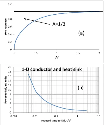
We now show, in Figure 3a, the integral of the normalized impulse response Z(t) from Fig. 2b, i.e., the step response to a constant power step. This function is
, (11)
which converges to 1 as shown. The delay time is characterized by the area in the upper left hand corner and is found to be, in normalized terms, 1/3. Thus a CAD measurement of step power response can be fit to this kind of impedance function by setting final temperature to 1 (giving a scaling factor Z0 from
Tfinal/P0) and multiplying the time delay area, as
shown, by 3 to give t*. The Elmore Delay [15] of 1/3
4
for this function represents the first moment of the impulse response, or
(12)
The relationship is most easily proven by going back to the s-domain expression for the shorted line Z(s) as in (3) and expanding tanh for the normalized function to give
(13)
with (minus) the s-coefficient being the delay time [15].
For finite line length, we have a heat sink, A=1 as in Fig. 2b, and thus for long enough time, t/t* will be large, the integral of Z(t) will be unchanging and thus the Dwyer power-time curve will be flat. This is of course the V=IR (or Tcrit=PcritZth) type of condition.
The transition from falling slope to flat power-time curve is captured by the integral of Z(t) out to various times. This is shown on a semilog plot in Figure 3.
Figure 3. (a) Integrated normalized Z(t) (step response) from Fig. 2b, showing convergence to 1 and Elmore Delay [15] of t*/3. (b) Semilog plot of Normalized Dwyer Curve based on 1D Heat Flow Model of Fig.1.
The normalized curve converges to 1 on the order of time constant t*, as expected. It is not clear how to
parameterize the plot, but the curve resembles other semilog Dwyer curve plots, as in [1]. A more enlightening view is seen in Figure 4, a log-log plot of the same data. While the W-B limit is at very short times, there is also a long section in the middle of the descending curve, more than a decade in time, which can be fit with a line and extrapolated to intercept the steady-state Pcrit() value at about t=0.79t*. Now we
have what we need to fit the entire curve, t* (a function of length, defined following Eq. (6)) and the steady state value Pcrit(). Then in accordance with
Eq. (9),
t crit crit
dt t
t t t P t
P
0 *
* 4
/ )) / ( (exp(
) ( )
(
’ (14)
and we have the entire Dwyer curve, with 4(q)
defined by (7a). Everything is normalized to the final value of Pcrit, but we can go to Eq. (6) and the
definition of t* to deduce Tcrit from estimates of length
l and thermal conductivity K, or some similar interrelationship. We certainly have Zth(t) to within a
scaling constant once we have t*.
Figure 4. Log-log plot of normalized Dwyer curve, or Eq. (9), showing power law in the mid-section, extrapolated to t=0.79t*. This is how to extract a characteristic time t* from plotted data.
Now we can return to the exponential power function, with decay constant (tau), and compare its peak power curve Ppk to the Dwyer constant power curve
with power P0 and pulse length t0. We take the derived
Zth(t) function as in Eq. (6) and convolve with the
exponential power function, point by point, to give the upper curve in Figure 5. Inasmuch as the exponential power calculation reduces to the Dawson integral in the W-B limit of Zth(t), as discussed earlier, we expect
the upper curve in Fig. 5 to be 2x0=1.848… above the
lower curve on the left-hand end. We do see that, but the trend continues up to around =t* and Ppk begins
the long process of converging to P0 for >>t*.
.
3
1
)
/
*
(exp(
*
0
4
1
dt
t
t
t
t
m
t s t s
st s
Znorm *
5
We can now apply these methods to some actual Dwyer curve device data as in [1], shown in Figure 6. The transition region between the two groups of data (covering almost two orders of magnitude of time) can now be filled in because we have a complete “reasonable” Dwyer curve after using the curve fits shown to arrive at Pfinal=7.062W and t*=110.14 sec.
The power law section is extrapolated to Pfinal (taken
at 1msec) and the intercept point is t=0.79t* as noted above.
Figure 5. Constant power P0 Dwyer curve (blue) vs. pulse length
t0 compared with peak power Ppk exponential curve (red) vs. time
constant , normalized to t*. Exponential curve calculated from convolution with Z(t) as in Eq. (6) and over most of its range is about 2x0=1.848… above the constant power curve as predicted
by the Dawson integral.
Figure 6. Dwyer curve device data as in Figure 12 of [1], taken with two different instruments.
The power law approximations from [1] as in Figure 6 are also pretty good, as we plot the Fig. 6 Dwyer curve log-log in Figure 7. After extracting Zth(t) using
Eq. (10), we convolve and plot the exponential power function (red) also, resembling Fig. 5. The red curve in Fig. 7 lies 1.75-1.95x above the blue curve in the sloped portion, generally as expected and in agreement with Fig. 5.
Figure 7: Dwyer curve (blue) plotted log-log from power laws in Fig. 6 [1]. Result for exponential power function (red) lies 1.75-1.95x higher over most of its range, as expected.
The step response of a square-shaped IC metal test pattern often gives near-perfect agreement with the Theta4-derived curves in Fig. 3 (normalized to t*, which tends to be in the sec) because it is nearly 1-D, describing low-K oxide between metal and high-K silicon. This is a worst case for given conditions and the curve is coincident with the Theta curve in Fig. 8. However, a long, narrow test pattern turns out, in FEM simulations, to deviate as in Figure 8 because of 2-D and ultimately 3-D heat spreading.
Figure 8. Constant power step response of a (long, narrow) IC metal test pattern, compared with the Theta4-derived step response as in Fig. 3. Plot is normalized to final temperature and t*. But many square metal slabs follow the red Theta curve because of their 1-D heat flow.
IV. Adiabatic Portion
6
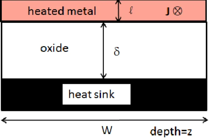
Figure 9. Metal on oxide with a heat sink, heated by electric current. Large values of W and z allow the 1-D approximation.
Figure 10. Electrical equivalent of metal on oxide with a heat sink, showing capacitive influence of bulk metal, and with I2R power
input as current source.
Up to now (as in Fig. 1) we have not considered the capacitive influence of the metal, and the W-B approximation does not consider it. But this capacitance, taken alone, is the adiabatic response, with impedance Zc(s)=1/sCmetal and admittance Yc(s)
the reciprocal. For an infinitely long line (Eq. 2a, Z0~1/√s) in parallel with the metal capacitance, the
admittances add. The total impedance is of the following form and transforms according to [11], 29.3.90:
)
(
)
(
1
)
(
Z
t
e
2erfc
a
t
s
a
s
s
Z
at
. (15)The quantity 1/a2 is a scaling time constant derivable
from the network, equal to Cmetal2/(KρCp), and it is
understood that Cmetal and ρCp are in units of
joules/ºC, K in W/ºC. This Z(t) (normalized; with scaling constant 1/Cmetal) approaches the adiabatic
constant value asymptotically for small times (step response a ramp going as τ), and becomes the W-B 1/√ at larger times. Indeed, the scheme of Fig. 10 for infinite line length has found application at this conference in several works on magnetoresistive sensors by Iben, in treatments of dynamic thermal conductance across the adiabatic and diffusion regimes [16, and references therein]. In these works,
thermal conductance is the parallel combination of time-dependent step responses, i.e., a harmonic average, resulting in a 1/τ + 1/√τ function (in reduced time units) for the conductance. The reciprocal of the integrated Z(t) function of Eq. (15) (step response turned into a conductance, not unlike Eq. (9)) is so close to this harmonic average function that it makes no difference which one is used for data-fitting. However, the mathematical rigor of Eq. (15), the true solution to the 1-D heat equation, should be recalled in other cases, for example a parallel R-C heat sink. The harmonic average normalized solution would give step response t/(1+t), which has the correct asymptotic limits but is not correct. The true step response of a (normalized) parallel R-C circuit is the inverse Laplace Transform of 1/[s(1+s)], or 1-exp(-t), an exponential and faster approach to 1.
A series expansion by Pierce ([17], Eq. 11) appears to solve exactly for the heat sunk line, at least as far as an integrated impedance, or step response, in time domain. This would solve for the case of Figs. 9-10 for any δ, adding admittances to get the form
)
coth(
1
)
(
s
k
s
a
s
s
Z
. (16)Proving that inversion of (16) is equivalent to [17], Eq. 11, is beyond the scope of this paper.
V. Discussion
The 1-D heat flow model with perfect heat sink located by a characteristic time constant is of course an idealized way to look at the kind of heat flow effects that allow the Zth(t) integral to converge and
the Dwyer curve to flatten out. Many of these effects relate to the ultimate 3-D nature of heat flow, whereby the flow out of a rectangular slab will at first seem one-dimensional (with W-B t-1/2 impulse response),
then if its aspect ratio is large there will be apparent 2-D heat flow (t-1 impulse response). But on a long
enough time scale, every heat source is a 3-D point source, with t-3/2 impulse response (the rule of thumb
is t-1/2 per dimension [9]) even into an infinitely deep
slab. The step response of these thermal impedances, i.e., the time integrals, will not converge for one (t1/2)
or two (ln t) dimensions, but will converge for three dimensions (t-1/2) once the point source effect takes
7
sink works remarkably well as a way to capture the various parts of the Dwyer curve with meaningful parameters.
These concepts can even be used to speed up computer calculations of heat flow. Suppose you have a 2-D transistor heat flow model that is computationally much faster than a complete 3-D model. The latter may better represent the real case but is slower. It requires judgement calls, but a few simulations could help equip the more interactive 2-D model with well-located artificial heat sink that better represents the 3-D effects that are felt at longer times. The effects can be bounded so that having the artificial sink is “no better than” having actual 3-D behavior, yet close. In this way, the iterative exploratory process (involving a human agent learning things from both 2-D and 3-D models) could be enhanced.
There can be other exercises in approximation to “bound” a problem and obtain a reasonably close heat flow solution using transmission line theory. While the case of the heat sink with finite resistance was not treated here, there is an interesting but little-known transformation [18] that could enlighten that and other heat flow and transmission line problems. The theorem of [18] applies to all RLGC transmission lines, not just lossy and lossless. Essentially, the theorem decomposes an arbitrarily terminated line into one of two series-parallel combinations, where all the transmission lines are open or shorted. In the case of heat flow, series approximations can be done more easily on the transformed lines in order to put bounds on the problem. Examples have been worked out but will have to wait for a future publication.
VI. Conclusions
This work began when the author noticed [8] that the Wunsch-Bell theorem [7] can be worked out in a line or two with RC transmission line theory and a table of Laplace Transforms. The next logical step was to go from the infinite line of W-B to a shorted one of finite length, likely to be a common and realistic situation when heat sinks are present. This too has a model in the s-domain and transformations to the time domain through Laplace Transforms, as described. A finite thermal impedance is of course the long-term step response of the shorted RC line, defining the flat part of the Dwyer curve, with the rest of the curve defined by the full expansion of the shorted line model. This complete view of 1-D heat flow for short and long lines was not captured in the groundbreaking work of Wunsch and Bell [7], but perhaps would have been had it been noticed. The key insight is analogy with
RC transmission lines and their impedances and admittances in the s-domain, with step and impulse responses invertible into in the time domain, through Laplace Transforms. The latter are certainly used in heat flow problems ([9, 17]) but the electrical transmission line analogy is more rarely invoked. This work has shown how to generate the heat impulse response function Z(t) for the 1-D shorted line as a fairly simple series expansion and how the nearly-complete Dwyer curve for constant power input emerges from that through integration. The commonly-observed adiabatic effect of resistively heated metal at short times can be captured too and blended with the rest of the Dwyer curve, through approximation. It is shown that when plotted log-log in power and time, the Dwyer curve has two easily extracted parameters, magnitude scaling and a characteristic time t*, that allow the entire curve to be filled in from a few data points. Another key use of the derived Z(t) function was to convolve with the often-used exponential decay power function [3-6] to generate its SOA curve, which in a certain range is shown, through a connection to the Dawson Integral, to lie (ideally) a factor of 1.848 above the constant-power Dwyer curve, in agreement with experimental work [3-6].
The issue of self-heating and feedback effects has not entered here but has been treated in the context of these same concepts elsewhere [8, 19] for metal heating. In these cases, the power input function has to be determined iteratively because of the self-heating effects, requiring repeated convolutions to determine a temperature waveform. These go fairly efficiently when the problem has been reduced to a 1-D type of model, but it was recently reported [19] that they can become far more efficient for double exponential ESD current inputs like HBM, charged device model (CDM), and probably other decaying pulses. Since the peak temperature is of interest, it was found in [19] that Tpeak itself follows a simple
scalar feedback equation with two parameters that emerge from a few simulations. The parameters are then linked to thermal and electrical properties and general trends discerned. Thus the Tpeak with nonlinear
feedback, due to self-heating, becomes far more predictable from fewer simulations.
Acknowledgments
8
author, please use the personal email at the head of this article.
References
[1] T. Smedes, Y. Christoforou, and S. Zhao, “Characterization Methods to Replicate EOS Fails”, Proc. EOS/ESD Symposium, vol. 36, pp. 384-392, 2014.
[2] A. Kamdem, P. Martin, J.-L. Lefebvre, F. Berthet, B. Domenges, and P. Guillot, “Electrical Overstress Robustness and Test Method for ICs”, Proc. EOS/ESD Symposium, vol. 36, pp. 393-399, 2014.
[3] F. Magrini and M. Mayerhofer, “Advanced Wunsch-Bell Based Application for Automotive Pulse Robustness Sizing”, Proc. EOS/ESD Symposium, vol. 36, pp. 400-407, 2014.
[4] V. M. Dwyer, A. J. Franklin, and D. S. Campbell, "Thermal Failure in Semiconductor Devices", Solid State Electronics, vol. 33. pp. 553-560, 1990.
[5] V. M. Dwyer, A. J. Franklin, and D. S. Campbell, “Electrostatic Discharge Thermal Failure in Semiconductor Devices”, IEEE Trans. Elec. Dev., vol. 37, no. 11, pp. 2381-87, Nov. 1990.
[6] D. G. Pierce, W. Shiley, B. D. Mulcahy, K. E. Wagner, and M. Wunder, "Electrical overstress testing of a 756K UVEPROM to rectangular and double exponential pulses," Proc. EOS/ESD Symp., vol. 10, pp. 137-146, 1988.
[7] D. C. Wunsch and R. R. Bell, "Determination of Threshold Failure Levels of Semiconductor Diodes and Transistors Due to Pulse Voltages," IEEE Trans. Nucl. Sci., NS-15, pp. 244-259, 1968.
[8] T. J. Maloney, L. Jiang, S. S. Poon, K. B. Kolluru, and AKM Ahsan, "Achieving Electrothermal Stability in Interconnect Metal During ESD Pulses", 2013 Int'l Reliability Physics Symposium, paper EL-1.
[9] H. S. Carslaw and J. C. Jaeger, Conduction of Heat in Solids, 2nd edition. Oxford, UK: Oxford University Press, 1959.
[10] S. Ramo, J. Whinnery, and T. Van Duzer, Fields and Waves in Communication Electronics. New York: John Wiley & Sons, 1965.
[11] M. Abramowitz and I. A. Stegun, Handbook of Mathematical Functions. New York: Dover Publications, 1965. Laplace Transform tables are in Sec. 29.
[12] R. N. Bracewell, The Fourier Transform and Its Applications, New York: McGraw-Hill, 1965.
[13] Web article,
http://functions.wolfram.com/EllipticFunctions/E llipticTheta4/.
[14] Web article,
http://mathworld.wolfram.com/DawsonsIntegral. [15] W.C. Elmore, “The Transient Analysis of Damped Linear Networks With Particular Regard to Wideband Amplifiers”, J. Appl. Phys. Vol. 19(1), pp. 55-63 (1948).
[16] I.E.T. Iben, "Dielectric Breakdown of TMR Sensors and the Role of Joule Heating", Proc. EOS/ESD Symposium, vol. 38, paper 2A.3, 2016.
[17] D. G. Pierce, “Modeling Metallization Burnout of Integrated Circuits”, Proc. EOS/ESD Symposium, vol. 4, pp. 56-61, 1982.
[18] Web article,
https://www.sites.google.com/site/esdpubs/docum ents/zin-yin-eqckt.pdf; T.J. Maloney, “Novel
Equivalent Circuit for Zin or Yin of an Arbitrarily Terminated Transmission Line”; first version
published at
http://emcesd.com/tt2012/tt081012.htm, August 2012.
[19] T.J. Maloney, “Modeling Feedback Effects in

![Figure 7: Dwyer curve (blue) plotted log-log from power laws in Fig. 6 [1]. Result for exponential power function (red) lies 1.75-1.95x higher over most of its range, as expected](https://thumb-us.123doks.com/thumbv2/123dok_us/8195316.2172576/5.918.469.831.568.779/figure-dwyer-plotted-result-exponential-function-higher-expected.webp)