Data Mining for the Masses - Free Computer, Programming, Mathematics, Technical Books, Lecture Notes and Tutorials

(1)

Data Mining

for the Masses

(2)

A Global Text Project Book

This book is available on Amazon.com.

(3)

DEDICATION

(4)

(5)

ACKNOWLEDGEMENTS

I would not have had the expertise to write this book if not for the assistance of many colleagues at various institutions. I would like to acknowledge Drs. Thomas Hilton and Jean Pratt, formerly of Utah State University and now of University of Wisconsin—Eau Claire who served as my Master’s degree advisors. I would also like to acknowledge Drs. Terence Ahern and Sebastian Diaz of West Virginia University, who served as doctoral advisors to me.

I express my sincere and heartfelt gratitude for the assistance of Dr. Simon Fischer and the rest of the team at Rapid-I. I thank them for their excellent work on the RapidMiner software product and for their willingness to share their time and expertise with me on my visit to Dortmund.

(12)

(13)

(14)

(15)

CHAPTER ONE:

INTRODUCTION TO DATA MINING AND CRISP-DM

INTRODUCTION

Data mining as a discipline is largely transparent to the world. Most of the time, we never even notice that it’s happening. But whenever we sign up for a grocery store shopping card, place a purchase using a credit card, or surf the Web, we are creating data. These data are stored in large sets on powerful computers owned by the companies we deal with every day. Lying within those data sets are patterns—indicators of our interests, our habits, and our behaviors. Data mining allows people to locate and interpret those patterns, helping them make better informed decisions and better serve their customers. That being said, there are also concerns about the practice of data mining. Privacy watchdog groups in particular are vocal about organizations that amass vast quantities of data, some of which can be very personal in nature.

The intent of this book is to introduce you to concepts and practices common in data mining. It is intended primarily for undergraduate college students and for business professionals who may be interested in using information systems and technologies to solve business problems by mining data, but who likely do not have a formal background or education in computer science. Although data mining is the fusion of applied statistics, logic, artificial intelligence, machine learning and data management systems, you are not required to have a strong background in these fields to use this book. While having taken introductory college-level courses in statistics and databases will be helpful, care has been taken to explain within this book, the necessary concepts and techniques required to successfully learn how to mine data.

(16)

particular is capable of many, many data mining tasks that are not covered in the book.

The chapters will all follow a common format. First, chapters will present a scenario referred to as

Context and Perspective. This section will help you to gain a real-world idea about a certain kind of

problem that data mining can help solve. It is intended to help you think of ways that the data mining technique in that given chapter can be applied to organizational problems you might face. Following Context and Perspective, a set of Learning Objectives is offered. The idea behind this section is that each chapter is designed to teach you something new about data mining. By listing the objectives at the beginning of the chapter, you will have a better idea of what you should expect to learn by reading it. The chapter will follow with several sections addressing the chapter’s topic. In these sections, step-by-step examples will frequently be given to enable you to work alongside an actual data mining task. Finally, after the main concepts of the chapter have been delivered, each chapter will conclude with a Chapter Summary, a set of Review Questions to help reinforce the main points of the chapter, and one or more Exercise to allow you to try your hand at applying what was taught in the chapter.

A NOTE ABOUT TOOLS

There are many software tools designed to facilitate data mining, however many of these are often expensive and complicated to install, configure and use. Simply put, they’re not a good fit for learning the basics of data mining. This book will use OpenOffice Calc and Base in conjunction with an open source software product called RapidMiner, developed by Rapid-I, GmbH of Dortmund, Germany. Because OpenOffice is widely available and very intuitive, it is a logical place to begin teaching introductory level data mining concepts. However, it lacks some of the tools data miners like to use. RapidMiner is an ideal complement to OpenOffice, and was selected for this book for several reasons:

 RapidMiner provides specific data mining functions not currently found in OpenOffice, such as decision trees and association rules, which you will learn to use later in this book.

 RapidMiner is easy to install and will run on just about any computer.

(17)

 Both RapidMiner and OpenOffice provide intuitive graphical user interface environments which make it easier for general computer-using audiences to the experience the power of data mining.

All examples using OpenOffice or RapidMiner in this book will be illustrated in a Microsoft Windows environment, although it should be noted that these software packages will work on a variety of computing platforms. It is recommended that you download and install these two software packages on your computer now, so that you can work along with the examples in the book if you would like.

OpenOffice can be downloaded from: http://www.openoffice.org/

RapidMiner Community Edition can be downloaded from: http://rapid-i.com/content/view/26/84/

THE DATA MINING PROCESS

Although data mining’s roots can be traced back to the late 1980s, for most of the 1990s the field was still in its infancy. Data mining was still being defined, and refined. It was largely a loose conglomeration of data models, analysis algorithms, and ad hoc outputs. In 1999, several sizeable companies including auto maker Daimler-Benz, insurance provider OHRA, hardware and software manufacturer NCR Corp. and statistical software maker SPSS, Inc. began working together to formalize and standardize an approach to data mining. The result of their work was CRISP-DM, the CRoss-Industry Standard Process for Data Mining. Although

(18)

Figure 1-1: CRISP-DM Conceptual Model.

CRISP-DM Step 1: Business (Organizational) Understanding

The first step in CRISP-DM is Business Understanding, or what will be referred to in this text as Organizational Understanding, since organizations of all kinds, not just businesses, can use data mining to answer questions and solve problems. This step is crucial to a successful data mining outcome, yet is often overlooked as folks try to dive right into mining their data. This is natural of course—we are often anxious to generate some interesting output; we want to find answers. But you wouldn’t begin building a car without first defining what you want the vehicle to do, and without first designing what you are going to build. Consider these oft-quoted lines from Lewis Carroll’s Alice’s Adventures in Wonderland:

"Would you tell me, please, which way I ought to go from here?" "That depends a good deal on where you want to get to," said the Cat. "I don’t much care where--" said Alice.

"Then it doesn’t matter which way you go," said the Cat.

"--so long as I get SOMEWHERE," Alice added as an explanation. "Oh, you’re sure to do that," said the Cat, "if you only walk long enough."

Indeed. You can mine data all day long and into the night, but if you don’t know what you want to know, if you haven’t defined any questions to answer, then the efforts of your data mining are less

(19)

How can I increase my per-unit profit margin? How can I anticipate and fix manufacturing flaws and thus avoid shipping a defective product? From there, you can begin to develop the more specific questions you want to answer, and this will enable you to proceed to …

CRISP-DM Step 2: Data Understanding

As with Organizational Understanding, Data Understanding is a preparatory activity, and sometimes, its value is lost on people. Don’t let its value be lost on you! Years ago when workers did not have their own computer (or multiple computers) sitting on their desk (or lap, or in their pocket), data were centralized. If you needed information from a company’s data store, you could request a report from someone who could query that information from a central database (or fetch it from a company filing cabinet) and provide the results to you. The inventions of the personal computer, workstation, laptop, tablet computer and even smartphone have each triggered moves away from data centralization. As hard drives became simultaneously larger and cheaper, and as software like Microsoft Excel and Access became increasingly more accessible and easier to use, data began to disperse across the enterprise. Over time, valuable data stores became strewn across hundred and even thousands of devices, sequestered in marketing managers’ spreadsheets, customer support databases, and human resources file systems.

(20)

Are there acronyms or abbreviations that are unknown or unclear? You may need to do some research in the Data Preparation phase of your data mining activities. Sometimes you will need to meet with subject matter experts in various departments to unravel where certain data came from, how they were collected, and how they have been coded and stored. It is critically important that you verify the accuracy and reliability of the data as well. The old adage “It’s better than nothing” does not apply in data mining. Inaccurate or incomplete data could be worse than nothing in a data mining activity, because decisions based upon partial or wrong data are likely to be partial or wrong decisions. Once you have gathered, identified and understood your data assets, then you may engage in…

CRISP-DM Step 3: Data Preparation

Data come in many shapes and formats. Some data are numeric, some are in paragraphs of text, and others are in picture form such as charts, graphs and maps. Some data are anecdotal or narrative, such as comments on a customer satisfaction survey or the transcript of a witness’s testimony. Data that aren’t in rows or columns of numbers shouldn’t be dismissed though— sometimes non-traditional data formats can be the most information rich. We’ll talk in this book about approaches to formatting data, beginning in Chapter 2. Although rows and columns will be one of our most common layouts, we’ll also get into text mining where paragraphs can be fed into RapidMiner and analyzed for patterns as well.

Data Preparation involves a number of activities. These may include joining two or more data sets together, reducing data sets to only those variables that are interesting in a given data mining exercise, scrubbing data clean of anomalies such as outlier observations or missing data, or re-formatting data for consistency purposes. For example, you may have seen a spreadsheet or database that held phone numbers in many different formats:

(555) 555-5555 555/555-5555

555-555-5555 555.555.5555

555 555 5555 5555555555

(21)

consistent as possible. Data preparation can help to ensure that you improve your chances of a successful outcome when you begin…

CRISP-DM Step 4: Modeling

A model, in data mining at least, is a computerized representation of real-world observations. Models are the application of algorithms to seek out, identify, and display any patterns or messages in your data. There are two basic kinds or types of models in data mining: those that classify and those that predict.

Figure 1-2: Types of Data Mining Models.

As you can see in Figure 1-2, there is some overlap between the types of models data mining uses. For example, this book will teaching you about decision trees. Decision Trees are a predictive model used to determine which attributes of a given data set are the strongest indicators of a given outcome. The outcome is usually expressed as the likelihood that an observation will fall into a certain category. Thus, Decision Trees are predictive in nature, but they also help us to classify our data. This will probably make more sense when we get to the chapter on Decision Trees, but for now, it’s important just to understand that models help us to classify and predict based on patterns the models find in our data.

(22)

All analyses of data have the potential for false positives. Even if a model doesn’t yield false positives however, the model may not find any interesting patterns in your data. This may be because the model isn’t set up well to find the patterns, you could be using the wrong technique, or there simply may not be anything interesting in your data for the model to find. The Evaluation phase of CRISP-DM is there specifically to help you determine how valuable your model is, and what you might want to do with it.

Evaluation can be accomplished using a number of techniques, both mathematical and logical in nature. This book will examine techniques for cross-validation and testing for false positives using RapidMiner. For some models, the power or strength indicated by certain test statistics will also be discussed. Beyond these measures however, model evaluation must also include a human aspect. As individuals gain experience and expertise in their field, they will have operational knowledge which may not be measurable in a mathematical sense, but is nonetheless indispensable in determining the value of a data mining model. This human element will also be discussed throughout the book. Using both data-driven and instinctive evaluation techniques to determine a model’s usefulness, we can then decide how to move on to…

CRISP-DM Step 6: Deployment

(23)

something no pollster or election insider consider likely, or even possible. In fact, most ‘experts’ expected Stevenson to win by a narrow margin, with some acknowledging that because they expected it to be close, Eisenhower might also prevail in a tight vote. It was only late that night, when human vote counts confirmed that Eisenhower was running away with the election, that CBS went on the air to acknowledge first that Eisenhower had won, and second, that UNIVAC had predicted this very outcome hours earlier, but network brass had refused to trust the computer’s prediction. UNIVAC was further vindicated later, when it’s prediction was found to be within 1% of what the eventually tally showed. New technology is often unsettling to people, and it is hard sometimes to trust what computers show. Be patient and specific as you explain how a new data mining model works, what the results mean, and how they can be used.

While the UNIVAC example illustrates the power and utility of predictive computer modeling (despite inherent mistrust), it should not construed as a reason for blind trust either. In the days of UNIVAC, the biggest problem was the newness of the technology. It was doing something no one really expected or could explain, and because few people understood how the computer worked, it was hard to trust it. Today we face a different but equally troubling problem: computers have become ubiquitous, and too often, we don’t question enough whether or not the results are accurate and meaningful. In order for data mining models to be effectively deployed, balance must be struck. By clearly communicating a model’s function and utility to stake holders, thoroughly testing and proving the model, then planning for and monitoring its implementation, data mining models can be effectively introduced into the organizational flow. Failure to carefully and effectively manage deployment however can sink even the best and most effective models.

DATA MINING AND YOU

(24)

(25)

CHAPTER TWO:

ORGANIZATIONAL UNDERSTANDING AND DATA

UNDERSTANDING

CONTEXT AND PERSPECTIVE

Consider some of the activities you’ve been involved with in the past three or four days. Have you purchased groceries or gasoline? Attended a concert, movie or other public event? Perhaps you went out to eat at a restaurant, stopped by your local post office to mail a package, made a purchase online, or placed a phone call to a utility company. Every day, our lives are filled with interactions – encounters with companies, other individuals, the government, and various other organizations.

In today’s technology-driven society, many of those encounters involve the transfer of information electronically. That information is recorded and passed across networks in order to complete financial transactions, reassign ownership or responsibility, and enable delivery of goods and services. Think about the amount of data collected each time even one of these activities occurs.

Take the grocery store for example. If you take items off the shelf, those items will have to be replenished for future shoppers – perhaps even for yourself – after all you’ll need to make similar purchases again when that case of cereal runs out in a few weeks. The grocery store must constantly replenish its supply of inventory, keeping the items people want in stock while maintaining freshness in the products they sell. It makes sense that large databases are running behind the scenes, recording data about what you bought and how much of it, as you check out and pay your grocery bill. All of that data must be recorded and then reported to someone whose job it is to reorder items for the store’s inventory.

(26)

trends as well. The store can target market to you by sending mailers with coupons for products you tend to purchase most frequently.

Now let’s take it one step further. Remember, if you can, what types of information you provided when you filled out the form to receive your frequent shopper card. You probably indicated your address, date of birth (or at least birth year), whether you’re male or female, and perhaps the size of your family, annual household income range, or other such information. Think about the range of possibilities now open to your grocery store as they analyze that vast amount of data they collect at the cash register each day:

 Using ZIP codes, the store can locate the areas of greatest customer density, perhaps aiding their decision about the construction location for their next store.

 Using information regarding customer gender, the store may be able to tailor marketing displays or promotions to the preferences of male or female customers.

 With age information, the store can avoid mailing coupons for baby food to elderly customers, or promotions for feminine hygiene products to households with a single male occupant.

These are only a few the many examples of potential uses for data mining. Perhaps as you read through this introduction, some other potential uses for data mining came to your mind. You may have also wondered how ethical some of these applications might be. This text has been designed to help you understand not only the possibilities brought about through data mining, but also the techniques involved in making those possibilities a reality while accepting the responsibility that accompanies the collection and use of such vast amounts of personal information.

LEARNING OBJECTIVES

After completing the reading and exercises in this chapter, you should be able to:

 Define the discipline of Data Mining

 List and define various types of data

(27)

 Explain some of the ethical dilemmas associated with data mining and outline possible solutions

PURPOSES, INTENTS AND LIMITATIONS OF DATA MINING

Data mining, as explained in Chapter 1 of this text, applies statistical and logical methods to large data sets. These methods can be used to categorize the data, or they can be used to create predictive

models. Categorizations of large sets may include grouping people into similar types of

classifications, or in identifying similar characteristics across a large number of observations.

Predictive models however, transform these descriptions into expectations upon which we can base decisions. For example, the owner of a book-selling Web site could project how frequently she may need to restock her supply of a given title, or the owner of a ski resort may attempt to predict the earliest possible opening date based on projected snow arrivals and accumulations.

It is important to recognize that data mining cannot provide answers to every question, nor can we expect that predictive models will always yield results which will in fact turn out to be the reality. Data mining is limited to the data that has been collected. And those limitations may be many. We must remember that the data may not be completely representative of the group of individuals to which we would like to apply our results. The data may have been collected incorrectly, or it may be out-of-date. There is an expression which can adequately be applied to data mining, among many other things: GIGO, or Garbage In, Garbage Out. The quality of our data mining results will directly depend upon the quality of our data collection and organization. Even after doing our very best to collect high quality data, we must still remember to base decisions not only on data mining results, but also on available resources, acceptable amounts of risk, and plain old common sense.

DATABASE, DATA WAREHOUSE, DATA MART, DATA SET…?

(28)

examine some of the variations in terminology used to describe data attributes.

Although we will be examining the differences between databases, data warehouses and data sets, we will begin by discussing what they have in common. In Figure 2-1, we see some data organized into rows (shown here as A, B, etc.) and columns (shown here as 1, 2, etc.). In varying data environments, these may be referred to by differing names. In a database, rows would be referred to as tuples or records, while the columns would be referred to as fields.

Figure 2-1: Data arranged in columns and rows.

In data warehouses and data sets, rows are sometimes referred to as observations, examples or cases, and columns are sometimes called variables or attributes. For purposes of consistency in this book, we will use the terminology of observations for rows and attributes for columns. It is important to note that RapidMiner will use the term examples for rows of data, so keep this in mind throughout the rest of the text.

(29)

Figure 2-2: A simple database with a relation between two tables.

Figure 2-2 depicts a relational database environment with two tables. The first table contains information about pet owners; the second, information about pets. The tables are related by the single column they have in common: Owner_ID. By relating tables to one another, we can reduce redundancy of data and improve database performance. The process of breaking tables apart and thereby reducing data redundancy is called normalization.

Most relational databases which are designed to handle a high number of reads and writes (updates and retrievals of information) are referred to as OLTP (online transaction processing) systems. OLTP systems are very efficient for high volume activities such as cashiering, where many items are being recorded via bar code scanners in a very short period of time. However, using OLTP databases for analysis is generally not very efficient, because in order to retrieve data from multiple tables at the same time, a query containing joins must be written. A query is simple a method of retrieving data from database tables for viewing. Queries are usually written in a language called SQL (Structured Query Language; pronounced ‘sequel’). Because it is not very useful to only query pet names or owner names, for example, we must join two or more tables together in order to retrieve both pets and owners at the same time. Joining requires that the computer match the Owner_ID column in the Owners table to the Owner_ID column in the Pets table. When tables contain thousands or even millions of rows of data, this matching process can be very intensive and time consuming on even the most robust computers.

(30)

a data warehouse. A data warehouse is a type of large database that has been denormalized and archived. Denormalization is the process of intentionally combining some tables into a single table in spite of the fact that this may introduce duplicate data in some columns (or in other words, attributes).

Figure 2-3: A combination of the tables into a single data set.

Figure 2-3 depicts what our simple example data might look like if it were in a data warehouse. When we design databases in this way, we reduce the number of joins necessary to query related data, thereby speeding up the process of analyzing our data. Databases designed in this manner are called OLAP (online analytical processing) systems.

Transactional systems and analytical systems have conflicting purposes when it comes to database speed and performance. For this reason, it is difficult to design a single system which will serve both purposes. This is why data warehouses generally contain archived data. Archived data are data that have been copied out of a transactional database. Denormalization typically takes place at the time data are copied out of the transactional system. It is important to keep in mind that if a copy of the data is made in the data warehouse, the data may become out-of-synch. This happens when a copy is made in the data warehouse and then later, a change to the original record (observation) is made in the source database. Data mining activities performed on out-of-synch observations may be useless, or worse, misleading. An alternative archiving method would be to move the data out of the transactional system. This ensures that data won’t get out-of-synch, however, it also makes the data unavailable should a user of the transactional system need to view or update it.

(31)

latter date format is adequate for the type of data mining being performed, it would make sense to simplify the attribute containing dates and times when we create our data set. Data sets may be made up of a representative sample of a larger set of data, or they may contain all observations relevant to a specific group. We will discuss sampling methods and practices in Chapter 3.

TYPES OF DATA

Thus far in this text, you’ve read about some fundamental aspects of data which are critical to the discipline of data mining. But we haven’t spent much time discussing where that data are going to come from. In essence, there are really two types of data that can be mined: operational and organizational.

The most elemental type of data, operational data, comes from transactional systems which record everyday activities. Simple encounters like buying gasoline, making an online purchase, or checking in for a flight at the airport all result in the creation of operational data. The times, prices and descriptions of the goods or services we have purchased are all recorded. This information can be combined in a data warehouse or may be extracted directly into a data set from the OLTP system.

(32)

data mart is an organizational data store, similar to a data warehouse, but often created in conjunction with business units’ needs in mind, such as Marketing or Customer Service, for reporting and management purposes. Data marts are usually intentionally created by an organization to be a type of one-stop shop for employees throughout the organization to find data they might be looking for. Data marts may contain wonderful data, prime for data mining activities, but they must be known, current, and accurate to be useful. They should also be well-managed in terms of privacy and security.

All of these types of organizational data carry with them some concern. Because they are secondary, meaning they have been derived from other more detailed primary data sources, they may lack adequate documentation, and the rigor with which they were created can be highly variable. Such data sources may also not be intended for general distribution, and it is always wise to ensure proper permission is obtained before engaging in data mining activities on any data set. Remember, simply because a data set may have been acquired from the Internet does not mean it is in the public domain; and simply because a data set may exist within your organization does not mean it can be freely mined. Checking with relevant managers, authors and stakeholders is critical before beginning data mining activities.

A NOTE ABOUT PRIVACY AND SECURITY

In 2003, JetBlue Airlines supplied more than one million passenger records to a U.S. government contractor, Torch Concepts. Torch then subsequently augmented the passenger data with additional information such as family sizes and social security numbers—information purchased from a data broker called Acxiom. The data were intended for a data mining project in order to develop potential terrorist profiles. All of this was done without notification or consent of passengers. When news of the activities got out however, dozens of privacy lawsuits were filed against JetBlue, Torch and Acxiom, and several U.S. senators called for an investigation into the incident.

(33)

have an ethical obligation to protect these individuals’ rights. This requires the utmost care in terms of information security. Simply because a government representative or contractor asks for data does not mean it should be given.

Beyond technological security however, we must also consider our moral obligation to those individuals behind the numbers. Recall the grocery store shopping card example given at the beginning of this chapter. In order to encourage use of frequent shopper cards, grocery stores frequently list two prices for items, one with use of the card and one without. For each individual, the answer to this question may vary, however, answer it for yourself: At what price mark-up has the grocery store crossed an ethical line between encouraging consumers to participate in frequent shopper programs, and forcing them to participate in order to afford to buy groceries? Again, your answer will be unique from others’, however it is important to keep such moral obligations in mind when gathering, storing and mining data.

The objectives hoped for through data mining activities should never justify unethical means of achievement. Data mining can be a powerful tool for customer relationship management, marketing, operations management, and production, however in all cases the human element must be kept sharply in focus. When working long hours at a data mining task, interacting primarily with hardware, software, and numbers, it can be easy to forget about the people, and therefore it is so emphasized here.

CHAPTER SUMMARY

(34)

REVIEW QUESTIONS

1) What is data mining in general terms?

2) What is the difference between a database, a data warehouse and a data set?

3) What are some of the limitations of data mining? How can we address those limitations?

4) What is the difference between operational and organizational data? What are the pros and cons of each?

5) What are some of the ethical issues we face in data mining? How can they be addressed?

6) What is meant by out-of-synch data? How can this situation be remedied?

7) What is normalization? What are some reasons why it is a good thing in OLTP systems, but not so good in OLAP systems?

EXERCISES

1) Design a relational database with at least three tables. Be sure to create the columns necessary within each table to relate the tables to one another.

2) Design a data warehouse table with some columns which would usually be normalized. Explain why it makes sense to denormalize in a data warehouse.

3) Perform an Internet search to find information about data security and privacy. List three web sites that you found that provided information that could be applied to data mining. Explain how it might be applied.

(35)

5) Using the Internet, locate a data set which is available for download. Describe the data set (contents, purpose, size, age, etc.). Classify the data set as operational or organizational. Summarize any requirements placed on individuals who may wish to use the data set.

(36)

(37)

CHAPTER THREE:

DATA PREPARATION

CONTEXT AND PERSPECTIVE

Jerry is the marketing manager for a small Internet design and advertising firm. Jerry’s boss asks him to develop a data set containing information about Internet users. The company will use this data to determine what kinds of people are using the Internet and how the firm may be able to market their services to this group of users.

To accomplish his assignment, Jerry creates an online survey and places links to the survey on several popular Web sites. Within two weeks, Jerry has collected enough data to begin analysis, but he finds that his data needs to be denormalized. He also notes that some observations in the set are missing values or they appear to contain invalid values. Jerry realizes that some additional work on the data needs to take place before analysis begins.

LEARNING OBJECTIVES

 Explain the concept and purpose of data scrubbing

 List possible solutions for handling missing data

 Explain the role and perform basic methods for data reduction

 Define and handle inconsistent data

 Discuss the important and process of attribute reduction

APPLYING THE CRISP DATA MINING MODEL

(38)

First, Jerry must ensure that he has developed a clear Organizational Understanding. What is the purpose of this project for his employer? Why is he surveying Internet users? Which data points are important to collect, which would be nice to have, and which would be irrelevant or even distracting to the project? Once the data are collected, who will have access to the data set and through what mechanisms? How will the business ensure privacy is protected? All of these questions, and perhaps others, should be answered before Jerry even creates the survey mentioned in the second paragraph above.

Once answered, Jerry can then begin to craft his survey. This is where Data Understanding enters the process. What database system will he use? What survey software? Will he use a publicly available tool like SurveyMonkey™, a commercial product, or something homegrown? If he uses publicly available tool, how will he access and extract data for mining? Can he trust this third-party to secure his data and if so, why? How will the underlying database be designed? What mechanisms will be put in place to ensure consistency and integrity in the data? These are all questions of data understanding. An easy example of ensuring consistency might be if a person’s home city were to be collected as part of the data. If the online survey just provides an open text box for entry, respondents could put just about anything as their home city. They might put New York, NY, N.Y., Nwe York, or any number of other possible combinations, including typos. This could be avoided by forcing users to select their home city from a dropdown menu, but considering the number cities there are in most countries, that list could be unacceptably long! So the choice of how to handle this potential data consistency problem isn’t necessarily an obvious or easy one, and this is just one of many data points to be collected. While ‘home state’ or ‘country’ may be reasonable to constrain to a dropdown, ‘city’ may have to be entered freehand into a textbox, with some sort of data correction process to be applied later.

(39)

understand that the examples of data preparation in this book are only a subset of possible data preparation approaches.

COLLATION

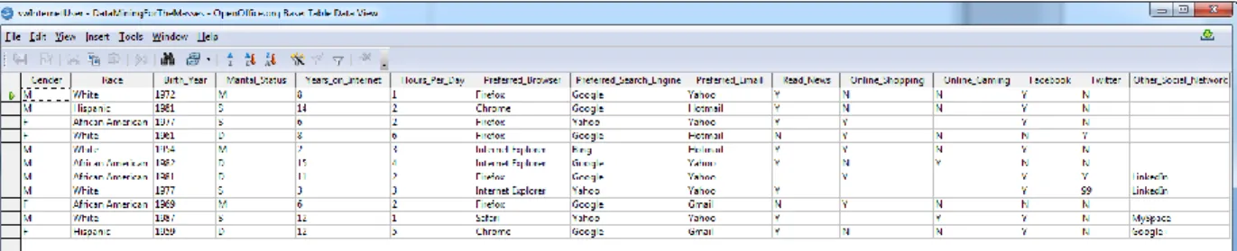
Suppose that the database underlying Jerry’s Internet survey is designed as depicted in the screenshot from OpenOffice Base in Figure 3-1.

Figure 3-1: A simple relational (one-to-one) database for Internet survey data.

This design would enable Jerry to collect data about people in one table, and data about their Internet behaviors in another. RapidMiner would be able to connect to either of these tables in order to mine the responses, but what if Jerry were interested in mining data from both tables at once?

(40)

Figure 3-2: Creation of a view in OpenOffice Base.

Figure 3-3: Results of the view from Figure 3-2 in datasheet view.

The creation of views is one way that data from a relational database can be collated and organized in preparation for data mining activities. In this example, although the personal information in the ‘Respondents’ table is only stored once in the database, it is displayed for each record in the ‘Responses’ table, creating a data set that is more easily mined because it is both richer in information and consistent in its formatting.

DATA SCRUBBING

(41)

HANDS ON EXERCISE

Starting now, and throughout the next chapters of this book, there will be opportunities for you to put your hands on your computer and follow along. In order to do this, you will need to be sure to install OpenOffice and RapidMiner, as was discussed in the section A Note about Tools in Chapter 1. You will also need to have an Internet connection to access this book’s companion web site, where copies of all data sets used in the chapter exercises are available. The companion web site is located at:

https://sites.google.com/site/dataminingforthemasses/

Figure 3-4. Data Mining for the Masses companion web site.

(42)

prepare data for mining in RapidMiner.

PREPARING RAPIDMINER, IMPORTING DATA, AND

HANDLING MISSING DATA

Our first task in data preparation is to handle missing data, however, because this will be our first time using RapidMiner, the first few steps will involve getting RapidMiner set up. We’ll then move straight into handling missing data. Missing data are data that do not exist in a data set. As you can see in Figure 3-5, missing data is not the same as zero or some other value. It is blank, and the value is unknown. Missing data are also sometimes known in the database world as null. Depending on your objective in data mining, you may choose to leave missing data as they are, or you may wish to replace missing data with some other value.

Figure 3-5: Some missing data within the survey data set.

The creation of views is one way that data from a relational database can be collated and organized in preparation for data mining activities. In this example, our database view has missing data in a number of its attributes. Black arrows indicate a couple of these attributes in Figure 3-5 above. In some instances, missing data are not a problem, they are expected. For example, in the Other Social Network attribute, it is entirely possible that the survey respondent did not indicate that they use social networking sites other than the ones proscribed in the survey. Thus, missing data are probably accurate and acceptable. On the other hand, in the Online Gaming attribute, there are answers of either ‘Y’ or ‘N’, indicating that the respondent either does, or does not participate in online gaming. But what do the missing, or null values in this attribute indicate? It is unknown to us. For the purposes of data mining, there are a number of options available for handling missing data.

(43)

1) Launch the RapidMiner application. This can be done by double clicking your desktop icon or by finding it in your application menu. The first time RapidMiner is launched, you will get the message depicted in Figure 3-6. Click OK to set up a repository.

Figure 3-6. The prompt to create an initial data repository for RapidMiner to use.

2) For most purposes (and for all examples in this book), a local repository will be sufficient. Click OK to accept the default option as depicted in Figure 3-7.

Figure 3-7. Setting up a local data repository.

(44)

Figure 3-8. Setting the repository name and directory.

(45)

Figure 3-9. Installing updates and adding the Text Mining module.

5) Once the updates and installations are complete, RapidMiner will open and your window should look like Figure 3-10:

(46)

on the ‘New’ icon as indicated by the black arrow in Figure 3-10. The resulting window should look like Figure 3-11.

Figure 3-11. Getting started with a new project in RapidMiner.

(47)

Figure 3-12. Adding a data set to a repository in RapidMiner.

(48)

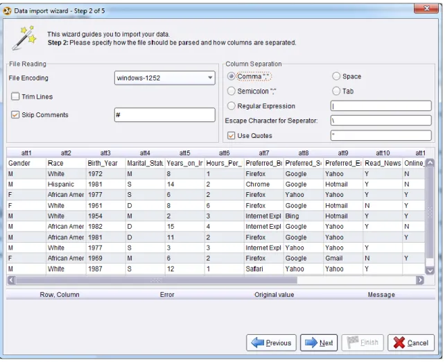
Figure 3-13. Importing a CSV file.

(49)

Figure 3-14. Locating the data set to import.

(50)

11)By default, RapidMiner looks for semicolons as attribute separators in our data. We must change the column separation delimiter to be Comma, in order to be able to see each attribute separated correctly. Note: If your data naturally contain commas, then you should be careful as you are collecting or collating your data to use a delimiter that does not naturally occur in the data. A semicolon or a pipe (|) symbol can often help you avoid unintended column separation.

Figure 3-16. A preview of attributes separated into columns with the Comma option selected.

(51)

Figure 3-17. Setting the attribute names.

(52)

Figure 3-18. Setting data types, roles and import attributes.

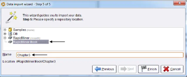
14)The final step is to choose a repository to store the data set in, and to give the data set a name within RapidMiner. In Figure 3-19, we have chosen to store the data set in the RapidMiner Book repository, and given it the name Chapter3. Once we click Finish, this data set will become available to us for any type of data mining process we would like to build upon it.

(53)

15)We can now see that the data set is available for use in RapidMiner. To begin using it in a RapidMiner data mining process, simply drag the data set and drop it in the Main Process window, as has been done in Figure 3-20.

Figure 3-20. Adding a data set to a process in RapidMiner.

(54)

Figure 3-21. Results perspective for the Chapter3 data set.

(55)

implications about the persons represented in each observation of our data set would be unfair and misrepresentative. Thus, we will change the missing values in the current example to illustrate how to handle missing values in RapidMiner, recognizing that what we are about to do won’t always be the right way to handle missing data. In order to have RapidMiner handle the change from missing to ‘N’ for the three observations in our Online_Gaming variable, click the design perspective icon.

Figure 3-22. Finding an operator to handle missing values.

(56)

click on the exa port on the Replace Missing Values operator. Exa stands for example set, and remember that ‘examples’ is the word RapidMiner uses for observations in a data set. Be sure the exa port from the Replace Missing Values operator is connected to your result set (res) port so that when you run your process, you will have output. Your model should now look similar to Figure 3-23.

Figure 3-23. Adding a missing value operator to the stream.

(57)

ones in Figure 3-24. Parameter settings that were changed are highlighted with black arrows.

Figure 3-24. Missing value parameters.

(58)

Figure 3-25. Results of changing missing data.

21)You can see now that the Online_Gaming attribute has been moved to the top of our list, and that there are zero missing values. Click on the Data View radio button, above and to the left hand side of the attribute list to see your data in a spreadsheet-type view. You will see that the Online_Gaming variable is now populated with only ‘Y’ and ‘N’ values. We have successfully replaced all missing values in that attribute. While in Data View, take note of how missing values are annotated in other variables, Online_Shopping for example. A question mark (?) denotes a missing value in an observation. Suppose that for this variable, we do not wish to replace the null values with the mode, but rather, that we wish to remove those observations from our data set prior to mining it. This is accomplished through data reduction.

DATA REDUCTION

Go ahead and switch back to design perspective. The next set of steps will teach you to reduce the number of observations in your data set through the process of filtering.

(59)

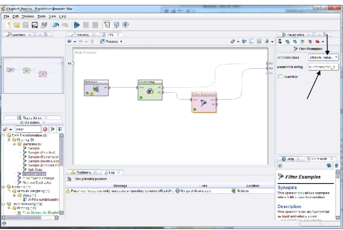
Filter Examples operator over and connect it into your stream, right after the Replace Missing Values operator. Your window will look like Figure 3-26.

Figure 3-26. Adding a filter to the stream.

(60)

Figure 3-27. Adding observation filter parameters.

Go ahead and run your model by clicking the play button. In results perspective, you will now see that your data set has been reduced from eleven observations (or examples) to nine. This is because the two observations where the Online_Shopping attribute had a missing value have been removed. You’ll be able to see that they’re gone by selecting the Data View radio button. They have not been deleted from the original source data, they are simply removed from the data set at the point in the stream where the filter operator is located and will no longer be considered in any downstream data mining operations. In instances where the missing value cannot be safely assumed or computed, removal of the entire observation is often the best course of action. When attributes are numeric in nature, such as with ages or number of visits to a certain place, an arithmetic measure of central tendency, such as mean, median or mode might be an acceptable replacement for missing values, but in more subjective attributes, such as whether one is an online shopper or not, you may be better off simply filtering out observations where the datum is missing. (One cool trick you can try in RapidMiner is to use the Invert Filter option in design perspective. In this example, if you check that check box in the parameters pane of the Filter Examples operator, you will keep the missing observations, and filter out the rest.)

(61)

processing time while testing a model to see if it will work to answer our questions. Follow the steps below to take a sample of our data set in RapidMiner.

1) Using the search techniques previously demonstrated, use the Operators search feature to find an operator called ‘Sample’ and add this to your stream. In the parameters pane, set the sample to be to be a ‘relative’ sample, and then indicate you want to retain 50% of your observations in the resulting data set by typing .5 into the sample ratio field. Your window should look like Figure 3-28.

Figure 3-28. Taking a 50% random sample of the data set.

2) When you run your model now, you will find that your results only contain four or five observations, randomly selected from the nine that were remaining after our filter operator removed records that had missing Online_Shopping values.

(62)

connected to the res port is also deleted. This is not a problem, you can reconnect the exa port from the Replace Missing Values operator to the res port, or you will find that the spline will reappear when you complete the steps under Handling Inconsistent Data.

HANDLING INCONSISTENT DATA

Inconsistent data is different from missing data. Inconsistent data occurs when a value does exist, however that value is not valid or meaningful. Refer back to Figure 3-25, a close up version of that image is shown here as Figure 3-29.

Figure 3-29. Inconsisten data in the Twitter attribute.

What is that 99 doing there? It seems that the only two valid values for the Twitter attribute should be ‘Y’ and ‘N’. This is a value that is inconsistent and is therefore meaningless. As data miners, we can decide if we want to filter this observation out, as we did with the missing Online_Shopping records, or, we could use an operator designed to allow us to replace certain values with others.

1) Return to design perspective if you are not already there. Ensure that you have deleted your sampling and filter operators from your stream, so that your window looks like Figure 3-30.

(63)

2) Note that we don’t need to remove the Replace Missing Values operator, because it is not removing any observations in our data set. It only changes the values in the Online_Gaming attribute, which won’t affect our next operator. Use the search feature in the Operators tab to find an operator called Replace. Drag this operator into your stream. If your splines had been disconnected during the deletion of the sampling and filtering operators, as is the case in Figure 3-30, you will see that your splines are automatically reconnected when you add the Replace operator to the stream.

(64)

Keep in mind that not all inconsistent data is going to be as easy to handle as replacing a single value. It would be entirely possible that in addition to the inconsistent value of 99, values of 87, 96, 101, or others could be present in a data set. If this were the case, it might take multiple replacements and/or missing data operators to prepare the data set for mining. In numeric data we might also come across data which are accurate, but which are also statistical outliers. These might also be considered to be inconsistent data, so an example in a later chapter will illustrate the handling of statistical outliers. Sometimes data scrubbing can become tedious, but it will ultimately affect the usefulness of data mining results, so these types of activities are important, and attention to detail is critical.

ATTRIBUTE REDUCTION

In many data sets, you will find that some attributes are simply irrelevant to answering a given question. In Chapter 4 we will discuss methods for evaluating correlation, or the strength of relationships between given attributes. In some instances, you will not know the extent to which a certain attribute will be useful without statistically assessing that attribute’s correlation to the other data you will be evaluating. In our process stream in RapidMiner, we can remove attributes that are not very interesting in terms of answering a given question without completely deleting them from the data set. Remember, simply because certain variables in a data set aren’t interesting for answering a certain question doesn’t mean those variables won’t ever be interesting. This is why we recommended bringing in all attributes when importing the Chapter 3 data set earlier in this chapter—uninteresting or irrelevant attributes are easy to exclude within your stream by following these steps:

(65)

Figure 3-32. Selecting a subset of a data set’s attributes.

(66)

keep. Suppose we were going to study the demographics of Internet users. In this instance, we might select Birth_Year, Gender, Marital_Status, Race, and perhaps Years_on_Internet, and move them to the right under Selected Attributes using the right green arrow. You can select more than one attribute at a time by holding down your control or shift keys (on a Windows computer) while clicking on the attributes you want to select or deselect. We could then click OK, and these would be the only attributes we would see in results perspective when we run our model. All subsequent downstream data mining operations added to our model will act only upon this subset of our attributes.

CHAPTER SUMMARY

This chapter has introduced you to a number of concepts related to data preparation. Recall that Data Preparation is the third step in the CRISP-DM process. Once you have established Organizational Understanding as it relates to your data mining plans, and developed Data Understanding in terms of what data you need, what data you have, where it is located, and so forth; you can begin to prepare your data for mining. This has been the focus of this chapter.

The chapter used a small and very simple data set to help you learn to set up the RapidMiner data mining environment. You have learned about viewing data sets in OpenOffice Base, and learned some ways that data sets in relational databases can be collated. You have also learned about comma separated values (CSV) files.

We have then stepped through adding CSV files to a RapidMiner data repository in order to handle missing data, reduce data through observation filtering, handle inconsistencies in data, and reduce the number of attributes in a model. All of these methods will be used in future chapters to prepare data for modeling.

(67)

may be misleading. Decisions based upon them could lead an organization down a detrimental and costly path. Learn to value the process of data preparation, and you will learn to be a better data miner.

REVIEW QUESTIONS

1) What are the four main processes of data preparation discussed in this chapter? What do they accomplish and why are they important?

2) What are some ways to collate data from a relational database?

3) For what kinds of problems might a data set need to be scrubbed?

4) Why is it often better to perform reductions using operators rather than excluding attributes or observations as data are imported?

5) What is a data repository in RapidMiner and how is one created?

6) How might inconsistent data cause later trouble in data mining activities?

EXERCISE

1) Locate a data set of any number of attributes and observations. You may have access to data sets through personal data collection or through your employment, although if you use an employer’s data, make sure to do so only by permission! You can also search the Internet for data set libraries. A simple search on the term ‘data sets’ in your favorite search engine will yield a number of web sites that offer libraries of data sets that you can use for academic and learning purposes. Download a data set that looks interesting to you and complete the following:

(68)

3) Import your data into your RapidMiner repository. Save it in the repository as Chapter3_Exercise.

4) Create a new, blank process stream in RapidMiner and drag your data set into the process window.

5) Run your process and examine your data set in both meta data view and Data View. Note if any attributes have missing or inconsistent data.

6) If you found any missing or inconsistent data, use operators to handle these. Perhaps try browsing through the folder tree in the Operators tab and experiment with some operators that were not covered in this chapter.

7) Try filtering out some observations based on some attibute’s value, and filter out some attributes.

(69)

(70)

(71)

CHAPTER FOUR:

CORRELATION

CONTEXT AND PERSPECTIVE

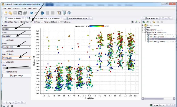
Sarah is a regional sales manager for a nationwide supplier of fossil fuels for home heating. Recent volatility in market prices for heating oil specifically, coupled with wide variability in the size of each order for home heating oil, has Sarah concerned. She feels a need to understand the types of behaviors and other factors that may influence the demand for heating oil in the domestic market. What factors are related to heating oil usage, and how might she use a knowledge of such factors to better manage her inventory, and anticipate demand? Sarah believes that data mining can help her begin to formulate an understanding of these factors and interactions.

LEARNING OBJECTIVES

 Explain what correlation is, and what it isn’t.

 Recognize the necessary format for data in order to perform correlation analysis.

 Develop a correlation model in RapidMiner.

 Interpret the coefficients in a correlation matrix and explain their significance, if any.

ORGANIZATIONAL UNDERSTANDING

(72)

DATA UNDERSTANDING

In order to investigate her question, Sarah has enlisted our help in creating a correlation matrix of six attributes. Working together, using Sarah’s employer’s data resources which are primarily drawn from the company’s billing database, we create a data set comprised of the following attributes:

 Insulation: This is a density rating, ranging from one to ten, indicating the thickness of each home’s insulation. A home with a density rating of one is poorly insulated, while a home with a density of ten has excellent insulation.

 Temperature: This is the average outdoor ambient temperature at each home for the most recent year, measure in degree Fahrenheit.

 Heating_Oil: This is the total number of units of heating oil purchased by the owner of each home in the most recent year.

 Num_Occupants: This is the total number of occupants living in each home.

 Avg_Age: This is the average age of those occupants.

 Home_Size: This is a rating, on a scale of one to eight, of the home’s overall size. The higher the number, the larger the home.

DATA PREPARATION

A CSV data set for this chapter’s example is available for download at the book’s companion web site (https://sites.google.com/site/dataminingforthemasses/). If you wish to follow along with the example, go ahead and download the Chapter04DataSet.csv file now and save it into your RapidMiner data folder. Then, complete the following steps to prepare the data set for correlation mining:

(73)

Figure 4-1. The chapter four data set added to the author’s RapidMiner Book repository.

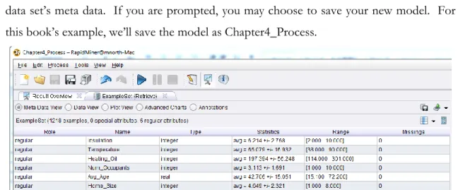
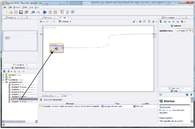
2) If your RapidMiner application is not open to a new, blank process window, click the new process icon, or click File > New to create a new process. Drag your Chapter4 data set into your main process window. Go ahead and click the run (play) button to examine the data set’s meta data. If you are prompted, you may choose to save your new model. For this book’s example, we’ll save the model as Chapter4_Process.

Figure 4-2. Meta Data view of the chapter four data set.

(74)

3) Switch back to design perspective. On the Operators tab in the lower left hand corner, use the search box and begin typing in the word correlation. The tool we are looking for is called Correlation Matrix. You may be able to find it before you even finish typing the full search term. Once you’ve located it, drag it over into your process window and drop it into your stream. By default, the exa port will connect to the res port, but in this chapter’s example we are interested in creating a matrix of correlation coefficients that we can analyze. Thus, is it important for you to connect the mat (matrix) port to a res port, as illustrated in Figure 4-3.

Figure 4-3. The addition of a Correlation Matrix to our stream, with the mat (matrix) port connected to a result set (res) port.

(75)

5) In Figure 4-4, we have our correlation coefficients in a matrix. Correlation coefficients are relatively easy to decipher. They are simply a measure of the strength of the relationship between each possible set of attributes in the data set. Because we have six attributes in this data set, our matrix is six columns wide by six rows tall. In the location where an attribute intersects with itself, the correlation coefficient is ‘1’, because everything compared to itself has a perfectly matched relationship. All other pairs of attributes will have a correlation coefficient of less than one. To complicate matters a bit, correlation coefficients can actually be negative as well, so all correlation coefficients will fall somewhere between -1 and 1. We can see that this is the case in Figure 4-4, and so we can now move on to the CRISP-DM step of…

EVALUATION

All correlation coefficients between 0 and 1 represent positive correlations, while all coefficients between 0 and -1 are negative correlations. While this may seem straightforward, there is an important distinction to be made when interpreting the matrix’s values. This distinction has to do with the direction of movement between the two attributes being analyzed. Let’s consider the relationship between the Heating_Oil consumption attribute, and the Insulation rating level attribute. The coefficient there, as seen in our matrix in Figure 4-4, is 0.736. This is a positive number, and therefore, a positive correlation. But what does that mean? Correlations that are positive mean that as one attribute’s value rises, the other attribute’s value also rises. But, a positive correlation also means that as one attribute’s value falls, the other’s also falls. Data analysts sometimes make the mistake in thinking that a negative correlation exists if an attribute’s values are decreasing, but if its corresponding attribute’s values are also decreasing, the correlation is still a positive one. This is illustrated in Figure 4-5.

Heating Oil use rises

Insulation rating also rises

Heating Oil use falls