Thermodynamic properties of hot nuclei within the self-consistent quasiparticle
random-phase approximation
N. Quang Hung1,*and N. Dinh Dang2,3,†
1Center for Nuclear Physics, Institute of Physics, Hanoi, Vietnam
2Theoretical Nuclear Physics Laboratory, RIKEN Nishina Center for Accelerator-Based Science,
2-1 Hirosawa, Wako City, 351-0198 Saitama, Japan
3Institute for Nuclear Science and Technique, Hanoi, Vietnam
(Received 15 July 2010; published 25 October 2010)
The thermodynamic properties of hot nuclei are described within the canonical and microcanonical ensemble approaches. These approaches are derived based on the solutions of the BCS and self-consistent quasiparticle random-phase approximation at zero temperature embedded into the canonical and microcanonical ensembles. The results obtained agree well with the recent data extracted from experimental level densities by the Oslo group for94Mo,98Mo,162Dy, and172Yb nuclei.
DOI:10.1103/PhysRevC.82.044316 PACS number(s): 21.60.Jz, 24.60.−k, 24.10.Pa
I. INTRODUCTION
Thermodynamic properties of highly excited (hot) nuclei have been a topic of much interest in nuclear physics. From the theoretical point of view, thermodynamic properties of any system can be studied by using three principal statistical ensembles, namely, the grand canonical ensemble (GCE), canonical ensemble (CE), and microcanonical ensemble (MCE). The GCE is an ensemble of identical systems in ther-mal equilibrium, which exchange their energies and particle numbers with an external heat bath. In the CE, the systems exchange only their energies, whereas their particle numbers are kept the same for all systems. The MCE describes thermally isolated systems with fixed energies and particle numbers. For convenience, the GCE is often used in most theoretical approaches, for example, the conventional finite-temperature BCS (FTBCS) theory [1], and/or finite-temperature Hartree-Fock-Bogoliubov theory [2]. These theories, however, fail to describe thermodynamic properties of finite small systems such as atomic nuclei or ultrasmall metallic grains. The reason is that the FTBCS theory neglects the quantal and thermal fluctuations, which have been shown to be very important in finite systems [3–8]. These fluctuations smooth out the superfluid-normal (SN) phase transition, which is a typical feature of infinite systems as predicted by the FTBCS theory.
Because an atomic nucleus is a system with fixed parti-cle number, partiparti-cle-number fluctuations are obviously not allowed. The use of the GCE in nuclear systems is therefore an approximation, which is good so long as the effects caused by particle-number fluctuations are negligible. The CE and MCE are often used in extending the exact solutions of the pairing Hamiltonian [8–10] to finite temperature, whereas the CE is preferred in the quantum Monte Carlo calculations at finite temperature (FTQMC) [11,12]. However, it is impracticable to find all the exact eigenvalues of the pairing Hamiltonian to construct the exact partition functions for large systems.
*[email protected] †[email protected]
For instance, in the half-filled doubly folded multilevel model (also called the Richardson model) withN =, whereis the number of single-particle levels andNthe number of particles, this cannot be done already for N > 14 [8,9]. In addition, the FTQMC method is quite time consuming and cannot be applied to heavy nuclei unless a limited configuration space is picked up. It is worth mentioning that the pairing Hamiltonian can also be solved exactly by using Richardson’s method, that is, by solving the Richardson equations. Using this method, the lowest eigenvalues of the pairing Hamiltonian can be obtained even for very large systems, for example, withN ==1000 (see, e.g., Ref. [13]). Nonetheless, these lowest eigenstates (obtained after solving the Richardson equations) are not sufficient for the construction of the exact partition function at finite temperature since the latter should contain all the excited states, not only the lowest ones. In principle, CE-based approaches can also be derived from an exact particle-number projection (PNP) at finite temperature on top of the GCE-based approaches [14]. However, this method is rather complicated for application to realistic nuclei.
level densities are first extrapolated to highE∗using the back-shifted Fermi-gas (BSFG) model. The CE partition function is then constructed, making use of the Laplace transformation of the level density. Knowing the partition function, one can calculate all the thermodynamic quantities within the CE, such as the free energy, total energy, heat capacity, and entropy. The thermodynamic quantities of the systems obtained within the MCE are calculated via Boltzmann’s definition of entropy. Although several experimental data for nuclear thermodynamic quantities extracted in this way by the Oslo group have recently been reported [18–21], most of the present theoretical approaches, derived within the GCE, cannot well describe these data, which are extracted within the CE and MCE. Recently, we have proposed a method that allowed us to construct theoretical approaches within the CE and MCE to describe rather well thermodynamic properties of atomic nuclei [22]. The proposed approaches are derived by solving the BCS and self-consistent quasiparticle RPA (SCQRPA) equations with the Lipkin-Nogami (LN) PNP for each total seniority S (number of unpaired particles at zero temperature) [23]. The results obtained are then embedded into the CE and MCE. Within the CE, the resulting approaches are called the CE-LNBCS and CE-LNSCQRPA, whereas they are called the MCE-LNBCS and MCE-LNSCQRPA within the MCE. The results obtained within these approaches are found in quite good agreement with not only the exact solutions of the Richardson model but also the experimentally extracted data for the 56Fe nucleus. The merit of these approaches resides in their simplicity and feasibility in application even to heavy nuclei, where the exact solution is impracticable and the FTQMC method is time consuming. The goal of the present article is to apply these approaches to describe microscopically the recently extracted thermodynamic quantities for94,96Mo, 162Dy, and172Yb nuclei.
The article is organized as follows. The pairing Hamiltonian and the derivations of the GCE-BCS, CE(MCE)-LNBCS, and CE(MCE)-LNSCQRPA equations are presented in Sec.II. The numerical results are analyzed and discussed in Sec.III, and the conclusions are drawn in the last section.
II. FORMALISM
A. Pairing Hamiltonian
The present article considers the pairing Hamiltonian
H =
kσ=±
kakσ† akσ −G
kk
ak†+ak†−ak−ak+, (1)
where akσ† and akσ are particle creation and destruction
operators on the kth orbitals, respectively. The subscripts k here imply the single-particle states in the deformed basis. This Hamiltonian describes a system ofNparticles (protons or neu-trons) interacting via a monopole pairing force with constant parameterG. The pairing Hamiltonian (1) can be diagonalized exactly by using the SU(2) algebra of angular momentum [10]. At finite temperatureT =0, the exact diagonalization is done for all total seniority or number of unpaired particles S because all excited states should be included in the exact
partition function. HereS=0,2, . . . , Nfor even-N systems, andS=1,3, . . . , N−1 for odd-N systems. For a system of N particles moving indegenerate single-particle levels, the numbernExact of exact eigenstatesEiExactS (iS=1, . . . , nExact)
obtained within exact diagonalization is given as nExact=
S
CS ×CN−S
pair−S/2, (2)
which combinatorially increases with N, where Cnm= m!/[n!(m−n)!] and Npair=N/2 [8]. Therefore, an exact
solution at T =0 is impossible for large-N systems, for example, N >14 for the half-filled case (N =), because of the huge size of the matrix to be diagonalized.
B. GCE-BCS approach
The well-known FTBCS approach to the pairing Hamilto-nian (1) is derived based on a variational procedure, which minimizes the grand potential
= H −TS−λN so that δ=0, (3) where S is the entropy of the system at temperatureT. The chemical potential λ is a Lagrangian multiplier, which can be obtained from the equation that maintains the expectation value of the particle-number operator equal to the particle number N. The expectation value O denotes the GCE average of the operator O [6] (Boltzmann’s constant kB is
set to 1),
O ≡ Tr[Oe−β(H−λN)]
Tre−β(H−λN) , β =
1
T. (4)
The conventional FTBCS equations for the pairing gapand particle numberN are then given as
=G
k
ukvk(1−2nk), N =2
k
(1−2nk)vk2+nk
,
(5) where the Bogoliubov coefficients uk,vk, the quasiparticle
energyEk, and the quasiparticle occupation numbernkhave
the usual forms: u2k = 1
2
1+k−Gv
2 k−λ Ek
,
v2k = 1 2
1−j −Gv
2 k−λ Ek
. (6)
Ek =
k−Gvk2−λ 2
+2, nk= 1
1+eβEk.
The systems of equations (5) and (6) are called the GCE-BCS equations. The total energy, heat capacity, and entropy obtained within the GCE-BCS approach are given by
E =2
k
(1−2nk)vk2+nk
−2
G −G
k
(1−2nk)v4k,
C = ∂E
∂T, S = −2
k
[nklnnk+(1−nk) ln(1−nk)].
C. CE-LNBCS
Unlike the GCE-BCS, the CE-LNBCS is derived based on the solutions of the BCS equations combined with the Lipkin-Nogami PNP [24] atT =0 for each total seniorityS of the system. When the pairs are broken, the unpaired particles denoted with the quantum numberskSblock the single-particle
levels k. As the result, these blocked single-particle levels do not contribute to the pairing correlation. Therefore, the LNBCS equations atT =0 can be derived by excluding these kSblocked levels. These equations are given as
LNBCS(kS)=G
k=kS
ukvk, N =2
k=ks
vk2+S, (8) where
u2k=k
S =
1 2
1+k−Gv
2
k−λ(kS) Ek
,
vk2=k
S =
1 2
1−k−Gv
2
k−λ(kS) Ek
, (9)
Ek=kS =
k−Gvk2−λ(kS) 2
+[LNBCS(k
S)]2, (10) λ(kS)=λ1(kS)+2λ2(kS)(N+1),
λ2(kS)= G
4
k=kSu
3
kvk k=kS ukvk3− k=kSu
4 kvk4
k=kSu
2 kv2k
2
− k=kSu
4 kvk4
. (11) As for the blocked single-particle levels,k=kS, their
occupa-tion numbers are always equal to 1/2. Solving the systems of Eqs. (8)–(11), one obtains the pairing gap LNBCS(k
S),
quasiparticle energiesEk, and Bogoliubov coefficientsukand vk, which correspond to each position of unpaired particles
on the blocked levelskS at each value of the total seniority S. There are nLNBCS= SC
S configurations of kS levels
distributed among single-particle levels at each value of S, which is also the number of eigenstates obtained within the LNBCS theory. The LNBCS energy (eigenvalue)EiLNBCSS for
each configuration is then given by
ELNBCS
iS =2
k=kS
kvk2+
kS
kS−
[LNBCS(k S)]2 G
−G
k=kS
vk4−4λ2(kS)
k=kS
u2kv2k. (12) The partition function of the so-called CE-LNBCS approach is constructed by using the LNBCS eigenvaluesELNBCS
iS as [22]
ZLNBCS(β)=
S dS
nLNBCS
iS=1
e−βEiSLNBCS, (13)
where dS=2S is the degeneracy. Knowing the partition
function (13), we can calculate all thermodynamic quantities of the system such as the free energyF, entropyS, total energy
E, and heat capacityCas follows: F = −TlnZ(T), S= −∂F
∂T, E=F +TS, C= ∂E ∂T. (14) The pairing gap is obtained by averaging the seniority-dependent gaps LNBCSi
S =
LNBCS(k
S) at T =0 in the CE
by means of the CE-LNBCS partition function (13), namely, CE-LNBCS=
1 ZLNBCS
S dS
nLNBCS
iS
LNBCSi
S e
−βELNBCS
iS . (15)
D. CE-LNSCQRPA
As mentioned previously in Sec. II A, a complete CE partition function should include all eigenstates. The LNBCS theory (atT =0) produces only the lowest eigenstates. For instance, for even (odd)Nthere is only one state atS=0(1), which is the ground state. ForS >0(1) there are also excited states in even (odd) systems, whose total numbernLNBCS is
much smaller thannExact. Consequently, the results obtained within the CE-LNBCS method can be compared with the exact ones only at low T, because at high T, higher eigenstates (excited states), which the LNBCS theory cannot reproduce, should be included in the CE partition function. This can be done by going beyond the quasiparticle mean field and introducing the LNSCQRPA, which incorporates not only the ground states but also the pairing vibrational excited states predicted by the QRPA [23]. The derivation of the LNSCQRPA equations has been presented in detail in Refs. [7,23,25], so we do not repeat it here. The LNSCQRPA formalism atT =0 for each total seniorityS proceeds in the same way as that of the LNBCS described in the previous section, namely, the LNSCQRPA equations are derived only for the unblocked levels k=kS, whereas the levels blocked by the unpaired
particlesk=kSdo not contribute to the pairing Hamiltonian.
The SCQRPA equation atT =0 has been derived in Ref. [23], and the final form reads
A B
B A
Xνk Yν k
=ων
Xνk
−Yν
k
. (16)
The SCQRPA submatrices are given by Akk =2
bk+2qkk+2
k
qkk(1−Dk)
− 1
Dk
k
dkk¯0|A†kAk|¯0
−2
k
hkk¯0|AkAk|¯0
δkk
+dkk
DkDk+8qkk
¯0|A†kAk|¯0
√
DkDk
, (17)
Bkk = −2
hkk+
1
Dk
k
dkk¯0|AkAk|¯0
+2
k
hkk¯0|A†kAk|¯0
δkk
+2hkk
DkDk+8qkk
¯0|AkAk|¯0
√
DkDk
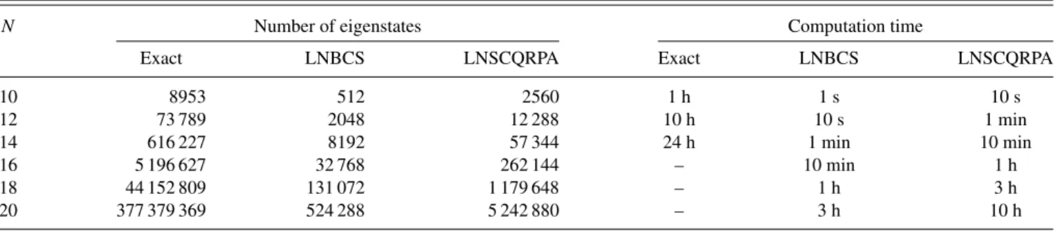
TABLE I. Number of eigenstates and computation time for the exact diagonalization of the pairing Hamiltonian as well as the numerical calculations within the CE-LNBCS and CE-LNSCQRPA for the doubly folded equidistant multilevel pairing model at several values ofN=. The computation time is estimated based on a shared large-memory computer Altix 450 with 512 gigabytes of memory in the RIKEN Integrated Cluster of Clusters (RICC) system.
N Number of eigenstates Computation time
Exact LNBCS LNSCQRPA Exact LNBCS LNSCQRPA
10 8953 512 2560 1 h 1 s 10 s
12 73 789 2048 12 288 10 h 10 s 1 min
14 616 227 8192 57 344 24 h 1 min 10 min
16 5 196 627 32 768 262 144 – 10 min 1 h
18 44 152 809 131 072 1 179 648 – 1 h 3 h
20 377 379 369 524 288 5 242 880 – 3 h 10 h
Ref. [23]. The screening factors¯0|A†kAk|¯0and¯0|AkAk|¯0,
withA†≡αk†α†−kthe creation operator of a two-quasiparticle pair, are given in terms of the SCQRPA amplitudesXkνandY
ν k
as
¯0|A†kAk|¯0 =
DkDk
ν
Yν kY
ν k,
(19)
¯0|AkAk|¯0 =
DkDk
ν
Xν kY
ν k,
where ¯0| · · · |¯0 denotes the expectation value in the SCQRPA ground state. The ground-state correlation factor
Dkis expressed in term of the backward-going amplitudesYkν
asDk=[1+2 ν(Y ν
k)2]−1with the sum running over all the
SCQRPA solutionsν.
After solving the LNSCQRPA equations (8) and (16)–(18) for each total seniority S, we obtain a set of eigenstates, consisting of the C
S lowest eigenstates (the ground state at S=0 or 1) as well as higher eigenstates (excited states) on top of these lowest ones, which come from the solutions of the LNSCQRPA equations with the eigenvalues ω(νS) (ν= 1, . . . , −S).1 As a result, the total number of eigenstates obtained within the LNSCQRPA is given by
nLNSCQRPA=
S
CS×(−S). (20) Consequently, the so-called CE-LNSCQRPA partition func-tion is calculated as
ZLNSCQRPA(β)=
S dS
nLNSCQRPA
iS=1
e−βEiSLNSCQRPA, (21)
which is formally identical to the CE-LNBCS partition func-tion (13), but the LNBCS eigenvaluesELNBCS
iS are now replaced
by EiLNSCQRPAS . From this partition function, the
thermody-namic quantities obtained within the CE-LNSCQRPA theory are calculated in the same way as those in Eq. (14). Although the numbernLNSCQRPAof the LNSCQRPA eigenstates is larger
1The SCQRPA has altogether−S+1 solutions with positive
energies. However, the lowest one corresponds to the spurious mode, whose energy is zero within the QRPA. Therefore it is excluded in the numerical calculations.
than nLNBCS, it is still much smaller than nExact. This most
important feature of the present method tremendously reduces the computing time in numerical calculations for heavy nuclei. As an example, we show in TableIthe number of eigenstates and the total executing time (the elapsed real time) for the exact diagonalization of the pairing Hamiltonian in CE-LNBCS and CE-LNSCQRPA calculations within the Richardson model at several values N of particle number, which is taken to be equal to the numberof single-particle levels (the half-filled case). This table shows that the execution time within the LNSCQRPA (LNBCS) is shorter than that consumed by exact diagonalization by about two (four) orders.
E. MCE-LNBCS and MCE-LNSCQRPA
The MCE entropy is calculated by using the Boltzmann definition
S(E)=lnW(E), W(E)=ρ(E)δE, (22) where ρ(E) is the density of states. In the LNBCS (LNSC-QRPA),W(E) is the number of LNBCS (LNSCQRPA) eigen-states within the energy interval (E,E+δE) [8]. Knowing the MCE entropy, one can calculate the MCE temperature as the first derivative of the MCE entropy with respect to the excitation energyE, namely,
T =
∂S(E) ∂E
−1
. (23)
The corresponding approaches, which embed the LNBCS and LNSCQRPA eigenvalues into the MCE, are called the MCE-LNBCS and MCE-LNSCQRPA, respectively.
F. Level density
The inverse relation of Eq. (22) reads
ρ(E)=eS(E)/δE, (24) which can be used to calculate the density of statesρ(E) from the fitted MCE entropy.
a result, the density of statesρ(E) at temperature T =β0−1, which corresponds to this minimum, is approximated as
ρ(E)≈Z(β0)eβ0E
2π∂
2lnZ(β 0)
∂β2 0
−1/2
≡eS(E)
−2π ∂E
∂β0
−1/2
, (25)
where Z(β0), S(E), and E are the CE partition function,
entropy, and total excitation energy of the systems, re-spectively. The density of states ρ(E) is obtained within the CE-LNBCS and CE-LNSCQRPA by replacing the par-tition function Z in Eq. (25) with that obtained within the CE-LNBCS in Eq. (13) and CE-LNSCQRPA in Eq. (21).
At finite angular momentumJ, in principle, the approach of LNSCQRPA plus angular momentum, which has been proposed by us in Ref. [27], should be used to calculate the angular-momentum-dependent level densityρ(E, M) with M being thezprojection of the total angular momentum. In this case the former doubly degenerate quasiparticle levels are resolved under the constraintM= kmk(n+k −n−k) with the
quasiparticle occupation numbersn±k, which are described by the Fermi-Dirac distribution n±k,FD= {exp[β(Ek∓γ mk)]+
1}−1 within the noninteracting quasiparticle approximation,
where mk is the spin projection of the kth single-particle
state |k,±mk,Ek is the quasiparticle energy, andγ is the
rotation frequency. Knowingρ(E, M), one can findρ(E, J)= ρ(E, M =J)−ρ(E, M=J+1) in the general case where the total angular momentum J is not aligned with the zaxis [28]. The total level densityρtot(E) and experimentally
observed level densityρobs(E), are then defined as [29] ρtot(E)=
J
(2J+1)ρ(E, J), ρobs(E)=
J
ρ(E, J). (26) The empirical entropySobs(E) is extracted from the observed
level densityρobs(E) in the same way as in Eq. (22), replacing ρ(E) withρobs(E), namely,
Sobs(E)=ln[ρobs(E)δE]. (27)
Because the present article considers nonrotating nuclei at low angular momentum, we assume thatρ(E, J)ρ(E,0)≡ ρ(E). Therefore, by fitting the MCE entropyS(E) in Eq. (22) to the experimentally observed entropySobs(E) in Eq. (27), that
is,S(E)Sobs(E), and inverting the result obtained by using
Eq. (24), what we get is actually a level density comparable to the experimentally observed one,ρobs(E)=exp[S(E)]/δE.
This means that the density of statesρ(E) calculated by using Eq. (24) or Eq. (25) without taking into account the effect of finite angular momentum is identical to the level density ρobs(E), not the total level density ρtot(E), because of the
absence of the factor (2J+1).
III. ANALYSIS OF NUMERICAL RESULTS
The proposed approaches are used to calculate the pairing gap, total energy, entropy, and heat capacity within the CE and MCE for a number of heavy isotopes, namely,94,98Mo,162Dy,
and172Yb.2 The single-particle energies are taken from the axially deformed Woods-Saxon potential with the depth of the central potential [30]
V =V0
1±kN−Z N+Z
, (28)
whereV0=51.0 MeV,k=0.86, and the plus and minus signs
stand for proton (Z) and neutron (N), respectively. The radius r0, diffusenessa, and spin-orbit strengthλare chosen to be
r0=1.27 fm, a=0.67 fm, and λ=35.0. The quadrupole deformation parametersβ2are estimated from the experimen-tal B(E2; 2+1 →0+1) values, and are 0.15, 0.17, 0.281, and 0.296 for 94Mo, 98Mo, 162Dy, and 172Yb, respectively [21]. The pairing interaction parameters G are adjusted so that the pairing gaps for neutrons and protons obtained within the LNSCQRPA at T =0 and S=0 reproduce the values extracted from the experimental odd-even mass differences, namely,N1.2, 1.0, 0.8, and 0.8 MeV for neutrons, and Z1.4, 1.3, 0.9, and 0.9 MeV for protons in94Mo,98Mo, 162Dy, and172Yb, respectively.
It is well known that pairing is significant only for the levels around the Fermi energy. Therefore, within the CE, we apply the same prescription proposed in Ref. [12] to calculate the CE partition function for medium and heavy isotopes. According to this prescription, we calculate the LNBCS and LNSCQRPA pairing gaps in the space spanned by 22 degenerate (proton or neutron) single-particle levels above the doubly magic48Ca
core for Mo isotopes; the same is done on top of the doubly magic 132Sn core for the Dy and Yb nuclei. The partition function obtained is then combined with those obtained within the independent-particle model (IPM) by using Eq. (15) of Ref. [12], namely,
lnZν=lnZν,tr+lnZsp −lnZsp,tr, (29) whereZν,tr ≡Zν,treβE0is the excitation partition function with
respect to the ground state energy E0 and Zν,tr is the CE
partition function obtained within the LNBCS [Eq. (13)] or LNSCQRPA [Eq. (21)] for 22 degenerate single-particle levels around the Fermi energy. Zsp is the CE partition function obtained within the IPM [see, e.g., Eq. (8) of Ref. [12]] for the space spanned by the levels from the bottom to theN =126 closed shell, whereasZsp,tr is the same partition function but for the truncated space spanned by 22 levels around the Fermi energy.
A. Results for molybdenum
Shown in Fig.1 are the pairing gaps, heat capacities and entropies for 94Mo [Figs. 1(a)–1(c)] and 98Mo [Figs. 1(d)–
1(f)] obtained within the LNBCS and CE(MCE)-LNSCQRPA versus the experimental data from Refs. [20] and [21]. There is a clear discrepancy in the heat capacities extracted from the same measured level density in these two
2See, e.g. Fig.1of Ref. [22] and the Appendix of the present article
5 10 15 20 25
0 0.2 0.4 0.6 0.8 1.0 1.2
C
T (MeV)
5 10 15 20
0 5 10 15 20
Mo
98
Z N
CE-LNBCS CE-LNSCQRPA
5 10 15 20 25
C
0 0.2 0.4 0.6 0.8 1.0 1.2
T (MeV)
5 10 15 20
0 5 10 15 20
Mo
94
Exp
0.2 0.4 0.6 0.8 1.0 1.2 1.4 1.6
∆
(MeV)
0.2 0.4 0.6 0.8 1.0 1.2 1.4 1.6
∆
(MeV)
∆(3)
MCE-LNBCS MCE-LNSCQRPA Exp (a)
(b)
(c)
(d)
(e)
(f)
FIG. 1. (Color online) Pairing gaps and heat capacities C obtained within the CE as functions ofT and entropiesSobtained within the MCE as functions ofE∗for94Mo (left panels) and98Mo
(right panels). In (a) and (d), the solid and dash-dotted lines denote the pairing gaps for protons and neutrons, respectively, whereas the thin and thick lines correspond to the CE-LNBCS and CE-LNSCQRPA results, respectively. In (b) and (e), the thin and thick solid lines stand for the CE-LNBCS and CE-LNSCQRPA results, whereas the thin and thick dash-dotted lines depict the experimental results taken from Refs. [20] and [21], respectively. Shown in (c) and (f) are the MCE entropies obtained within the MCE-LNBCS (squares) and MCE-LNSCQRPA (triangles), and extracted from experimental data (circles with error bars) of Ref. [20].
papers [Figs.1(b)and1(e)]. The heat capacity, extracted in Ref. [21], clearly shows a pronounced peak atT ∼0.7 MeV for both94Mo and98Mo, whereas the corresponding quantity,
extracted in Ref. [20], shows no trace of any peak. The source of the discrepancy is the difference in the scale of the excitation energyE∗that was used for extrapolating the measured level density before evaluating the CE partition function using the Laplace transformation of the level density. In Ref. [20], the level density is extrapolated up toE∗∼40–50 MeV, whereas in Ref. [21] this is done up to E∗=180 MeV. Given that all the excited states should be included in the partition function, the energy E∗ ∼40–50 MeV used in Ref. [20] seems to be too low, which might affect the resulting heat capacity. As Figs. 1(b) and 1(e) show, the heat capacities predicted by the CE-LNSCQRPA are much closer to those obtained in Ref. [21]. They are also consistent with the FTQMC calculations for other nuclei [11,12]. It is important to emphasize here that quantal and thermal fluctuations within the CE-LNBCS(LNSCQRPA) indeed smooth out the SN phase transition. As a result, the pairing gaps [Figs. 1(a)
and 1(d)] obtained for protons (solid lines) and neutrons (dash-dotted lines) within both the CE-LNBCS (thin lines) and CE-LNSCQRPA (thick lines) do not collapse at the critical temperature T =Tcof the SN phase transition, as predicted
by the GCE-BCS approach, but monotonically decrease with increasingT. The neutron gap in Fig.1(a)obtained within the CE-LNSCQRPA for 94Mo (thick dash-dotted lines) is close to the three-point gap (dashed lines) obtained in Ref. [21] by simply extrapolating the odd-even mass formula to finite temperature. As has been pointed out in Ref. [8], such a naive extrapolation contains the admixture with a contribution from uncorrelated single-particle configurations, which do not contribute to the pairing correlation. Therefore, to avoid obviously wrong results at high T, this contribution should be removed from the total energy of the system. Nonetheless, in the low-temperature region (T <1.3 MeV), as considered here, where the contribution of uncorrelated single-particle configurations is expected to be small, the simple extension of the three-point odd-even mass formula toT =0 can still serve as a useful indicator.
As has been discussed in Ref. [22], at lowE∗the genuine thermodynamic observable is the MCE entropy because it is calculated directly from the observable level density by using the Boltzmann definition (22). The experimental MCE entropies for 94,98Mo are plotted in Figs. 1(c) and 1(f)
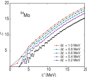
along with the predictions by the LNBCS and MCE-LNSCQRPA. These figures show that the MCE-LNSCQRPA results fit the available experimental data remarkably well. It is worth mentioning that the results obtained within the MCE-LNBCS(LNSCQRPA) are sensitive to the choice of energy intervalδE, which is used to calculate the number of accessible statesW(E) in Eq. (22). Figure2shows the entropies obtained within the CE-LNSCQRPA for94Mo using several values of
δEranging from 0.2 MeV to 1.0 MeV. It is clear from this figure that the MCE entropies increase withδE. In this respect, we found that the values ofδE =1 MeV for94Mo and 0.7 MeV for 98Mo are reasonable to fit the experimental data. The reason
for choosing large values of δE for these two nuclei comes
5 10 15 20
0 5 10 15 20 Mo
94
= 1.0 MeV δε
= 0.8 MeV δε
= 0.6 MeV δε
= 0.4 MeV δε
= 0.2 MeV δε
FIG. 2. (Color online) Microcanonical entropy as function ofE∗ obtained within the MCE-LNSCQRPA for94Mo using various values
from the deficiency of the CE-LNSCQRPA(LNBCS), which includes only low-lying excited states.
B. Results for dysprosium and ytterbium
The results obtained for 162Dy and 172Yb are shown
in Fig. 3. Similar to the results for 94,98Mo, the CE heat capacities and MCE entropies obtained within the CE(MCE)-LNSCQRPA for both162Dy and172Yb are in good agreement
with the experimental data. The neutron and proton gaps obtained within the CE-LNBCS(LNSCQRPA) do not collapse atT =Tcbut decrease with increasingT and remain finite at
highT even for the two heavy nuclei considered here. The peak in the experimental heat capacity nearT =0.4 MeV is seen in 172Yb, whereas it disappears in 162Dy. This is again
because the measured level densities for these two nuclei are extrapolated only up toE∗ =40 MeV instead of 180 MeV as was done in Ref. [21] for other nuclei. This is confirmed by the heat capacities obtained within the CE-LNSCQRPA (thick solid lines), which clearly show a peak aroundT =0.4 MeV.
0.2 0.4 0.6 0.8 1.0
∆
(MeV)
Yb
172
5 10 15 20 25 30 35
C
0 0.2 0.4 0.6 0.8 1.0 T (MeV)
5 10 15 20 25
0 5 10 15 20
0.2 0.4 0.6 0.8 1.0 1.2
T (MeV)
0 2 4 6 8 10
0.2 0.4 0.6 0.8 1.0
0 0.2 0.4 0.6 0.8 1.0 T (MeV) 5
10 15 20 25 30 35
C
∆
(MeV)
5 10 15 20 25
0 5 10 15 20
0.2 0.4 0.6 0.8 1.0 1.2
0 2 4 6 8 10
T (MeV)
Dy
162
Z N
CE-LNBCS CE-LNSCQRPA Exp
MCE-LNBCS MCE-LNSCQRPA Exp
(a)
(b)
(c)
(d)
(e)
(f)
(g)
(h)
FIG. 3. (Color online) (a), (b), (e), and (f): Pairing gaps, heat capacitiesCas functions ofT obtained within the CE; (c), (d), (g), and (h): EntropiesSand temperaturesT as functions ofE∗obtained within the MCE for 162Dy (left panels) and 172Yb (right panels).
Notations are the same as those in Fig.1. Experimental data are taken from Ref. [19].
In Figs. 3(d) and 3(h), one can see that the MCE tem-peratures, extracted from the experimental data (circles with error bars) by using Eq. (23), scatter around the experimental (thick dash-dotted lines) or theoretical (thick and thin lines) CE results. The results of calculations with the MCE-LNBCS (squares) and MCE-LNSCQRPA (triangles) by using the same definition (23) andδE =0.5 also describe these values well. The results for MCE entropies in Figs. 1 and 3 show the importance of the effect beyond the quasiparticle mean field included in the self-consistent coupling to QRPA vibrations. In fact, the MCE-LNSBCS results for the entropy clearly underestimate the experimental values. The discrepancy with the MCE-LNSCQRPA results increases withE∗to reach about 20% atE∗=20 MeV.
C. Level density
The level densities obtained within the CE-LNSCQRPA using Eq. (25) and MCE-LNSCQRPA using Eq. (24) are plotted in Fig. 4 as functions of excitation energy E∗ in comparison with the experimental data [19,20]ρobs(E)=ρ0×
exp[Sobs(E)]. In the latterρ0 is a normalization factor, which
should be put equal to 1/δE according to Eq. (27). However, because of fluctuations in level spacings, which make the entropy sensitive toδE, the authors of Ref. [19,20] chose the values ofρ0 to obtain entropySobs=0 atT =0. In this way
the value of ρ0 is set to 1.5 MeV−1 for 94,98Mo [20] and
3 MeV−1 for162Dy and172Yb [19]. Figure4 shows that the
level densities obtained within the MCE-LNSCQRPA offer the best fit to the experimental data for all nuclei under consid-eration. The results obtained within the CE-LNSCQRPA are closer to the experimental data for94,98Mo atE∗4 MeV, whereas at higherE∗ the MCE-LNSCQRPA offers a better performance. The S shape in the MCE-LNSCQRPA level density at lowE∗ might have come from the fixed value of the energy intervalδE, within which the levels are counted, according to the definition (22), whereas the denominator in
Mo
94
1 10 10 10 10 10 106
5
4
3
2
CE-LNSCQRPA
(a)
Exp
ρ
(MeV )
-1
MCE-LNSCQRPA
Mo
98
(b)
1 10 10 10 10 105
4
3
2
ρ
(MeV )
-1
1 10 10 10 108
6
4
2
ρ
(MeV )
-1
Dy
162
(c)
Yb
172
(d)
1 10 10 106
4
2
ρ
(MeV )
-1
0 2 4 6 8 10 0 2 4 6 8 10
FIG. 4. (Color online) Level densities as functions ofE∗obtained within the CE-LNSCQRPA (solid line) and MCE-LNSCQRPA (triangles) versus the experimental data (circles with error bars) for
2 4 6 8 10
0 10 20 30 40
1 10 10 10
2 3
ρ
(MeV )
-1
2 4 6 8 10
1 10 10 10
2 3
ρ
(MeV )
-1
0 10 20 30 40
N= =14
=1 MeV Ω
δ
ε
(a)(b)
(c)
(d)
=5 MeV δ
ε
FIG. 5. (Color online) MCE entropies and level densities as functions of E∗ obtained within the MCE-LNBCS (squares) and MCE-LNSCQRPA (triangles) versus the exact results for the
Richardson model (circles) with N==14 and G=1 MeV.
Results obtained by using the energy binδE=1 MeV are shown in (a) and (b), whereas those obtained by usingδE=5 MeV are shown in (c) and (d). Lines connecting the squares and triangles are drawn to guide the eye.
the definition of the CE level density [at the right-hand side of Eq. (25)] depends on E∗. A larger value ofδE at E∗ 4 MeV would eventually increase the MCE-LNSCQRPA level density, improving the agreement with the observed level density in this region, but there is no physical justification for doing this. The discrepancy between the CE-LNSCQRPA and experimental results seems to be larger and increases withE∗ for 162Dy and172Yb. This might be caused by the
absence of the contribution of higher multipolarities such as dipole, quadrupole, etc., which are not included in the present study and may be important for rare-earth nuclei. The use of SCQRPA plus angular momentum [27], discussed previously, may also improve the agreement.
IV. CONCLUSIONS
The present article applies the canonical and microcanon-ical ensembles of the LNBCS and LNSCQRPA, derived in Ref. [22], to describe the thermodynamic properties as well as level densities of several nuclei, namely, 94,98Mo, 162Dy,
and 172Yb. The results obtained show that the
CE(MCE)-LNSCQRPA describe quite well the recent experimental level densities and the thermodynamic quantities extracted for these nuclei by the Oslo group [18–21]. They confirm that the SN phase transition is smoothed out in nuclear systems because of the effects of quantal and thermal fluctuations, leading to a nonvanishing pairing gap at finite temperature even in heavy nuclei [3–8]. The discrepancy between the heat capacities obtained within the two different experimental works, which extrapolate the same experimental level density to different excitation energies, is also discussed. The heat capacities obtained within the CE-LNBCS(LNSCQRPA) for all nuclei
show a pronounced peak at T ∼Tc, whereas the results
extracted from the same experimental data by Refs. [20] and [21] show different behaviors. The better agreement between the predictions of our approaches as well as those of the FTQTMC and the results of Ref. [21] gives a strong indication of the fact that, to construct an adequate partition function for a good description of thermodynamic quantities, the measured level density should be extended up to very high excitation energy E∗ ∼180 MeV or 200 MeV. The small differences between the CE(MCE)-LNBCS(LNSCQRPA) results and the experimental data might be caused by the absence of the con-tribution of higher multipolarities such as dipole, quadrupole, etc., which are not included in the present study. In order to tackle this issue, the LNSCQRPA plus angular momentum [27] should be used and extended to included also the multipole residual interactions higher than the monopole pairing force. This task remains one of the subjects of our study in the future.
ACKNOWLEDGMENTS
The numerical calculations were carried out using the
FORTRAN IMSL Library by Visual Numerics on the RIKEN
Integrated Cluster of Clusters (RICC) system. A part of this work was carried out during the stay of N.Q.H. in RIKEN under support by a postdoctoral grant from the Nishina Memorial Foundation and by the Theoretical Nuclear Physics Laboratory of the RIKEN Nishina Center.
APPENDIX: MCE RESULTS WITHIN THE RICHARDSON MODEL
[1] J. Bardeen, L. Cooper, and Schrieffer, Phys. Rev.108, 1175 (1957);M. Sano and S. Yamasaki,Prog. Theor. Phys.29, 397 (1963).
[2] K. Tanabe and K. Sugaware-Tanabe, Phys. Lett. B 97, 337 (1980); A. L. Goodman, Nucl. Phys. A 352, 30 (1981); K. Tanabe, K. Sugaware-Tanabe, and H. J. Mang,ibid.357, 20 (1981); 357, 45 (1981).
[3] L. G. Moretto,Phys. Lett. B40, 1 (1972);A. L. Goodman,Phys. Rev. C29, 1887 (1984);J. L. Egido, P. Ring, S. Iwasaki, and H. J. Mang,Phys. Lett. B154, 1 (1985).
[4] R. Rossignoli, P. Ring, and N. D. Dang,Phys. Lett. B297, 9 (1992);N. D. Dang, P. Ring, and R. Rossignoli,Phys. Rev. C 47, 606 (1993).
[5] V. Zelevinsky, B. A. Brown, N. Frazier, and M. Horoi,Phys. Rep.276, 85 (1996).
[6] N. Dinh Dang and V. Zelevinsky, Phys. Rev. C 64, 064319 (2001);N. Dinh Dang and A. Arima,ibid.67, 014304 (2003); 68, 014318 (2003);N. D. Dang,Nucl. Phys. A784, 147 (2007). [7] N. Dinh Dang and N. Quang Hung,Phys. Rev. C77, 064315
(2008).
[8] N. Q. Hung and N. D. Dang,Phys. Rev. C79, 054328 (2009). [9] T. Sumaryada and A. Volya,Phys. Rev. C76, 024319 (2007). [10] R. W. Richardson,Phys. Lett.3, 277 (1963); 14, 325 (1965);
A. Volya, B. A. Brown, and V. Zelevinsky,Phys. Lett. B509, 37 (2001).
[11] S. Liu and Y. Alhassid,Phys. Rev. Lett.87, 022501 (2001) [12] Y. Alhassid, G. F. Bertsch, and L. Fang,Phys. Rev. C68, 044322
(2003).
[13] J. Dukelsky, S. Pittel, and G. Sierra,Rev. Mod. Phys.76, 643 (2004).
[14] R. Rossignoli and P. Ring,Ann. Phys. (NY)235, 350 (1994); R. Rossignoli, P. Ring, and N. D. Dang,Phys. Lett. B 297, 9 (1992);K. Tanabe and H. Nakada,Phys. Rev. C71, 024314 (2005);H. Nakada and K. Tanabe,ibid.74, 061301(R) (2006). [15] R. Rossignoli, N. Canosa, and P. Ring,Phys. Rev. Lett.80, 1853
(1998).
[16] K. Kaneko and A. Schiller,Phys. Rev. C75, 044304 (2007); 76, 064306 (2007).
[17] R. Rossignoli,Phys. Rev. C54, 1230 (1996).
[18] E. Melbyet al.,Phys. Rev. Lett.83, 3150 (1999);A. Schiller et al.,Phys. Rev. C63, 021306(R) (2001);E. Alginet al.,ibid.
78, 054321 (2008).
[19] M. Guttormsenet al.,Phys. Rev. C62, 024306 (2000). [20] R. Chankovaet al.,Phys. Rev. C73, 034311 (2006). [21] K. Kanekoet al.,Phys. Rev. C74, 024325 (2006).
[22] N. Q. Hung and N. D. Dang, Phys. Rev. C 81, 057302
(2010).
[23] N. Q. Hung and N. D. Dang,Phys. Rev. C76, 054302 (2007); 77, 029905(E) (2008).
[24] H. J. Lipkin,Ann. Phys. (NY)9, 272 (1960);Y. Nogami,Phys. Lett.15, 4 (1965).
[25] N. Dinh Dang and N. Quang Hung,Phys. Rev. C81, 034301 (2010).
[26] T. Ericson, Adv. Phys.9, 425 (1960).
[27] N. Q. Hung and N. D. Dang,Phys. Rev. C78, 064315 (2008). [28] A. Bohr and B. R. Mottelson, Nuclear Structure(Benjamin,
New York, 1969), Vol. 1.
[29] A. Gilbert and A. G. W. Cameron, Can. J. Phys. 43, 1446 (1965).