ECE35_SP17_HW02_Solution.pdf

ECE 35

Homework #2 Solution (Fall 2017, Taur)

All homework problems come from the textbook, “Introduction to Electric Circuits”, by Svoboda & Dorf, 9th Edition.

P 3.2-3 Consider the circuit shown in Figure P 3.2-3.

(a) Suppose that R1 = 8 Ω and R2 = 4 Ω. Find the current i and the voltage v.

(b) Suppose, instead, that i = 2.25 A and v = 42 V. Determine the resistances R1 and R2. (c) Suppose, instead, that the voltage source supplies 24 W of power and that the current source

supplies 9 W of power. Determine the current i, the voltage v, and the resistances R1 and R2.

Figure P 3.2-3

Solution:

2

2 2

1

1 1

KVL : 12 (3) 0 (outside loop)

12 12 3 or

3 12

KCL 3 0 (top node)

12 12

3 or

3

R v

v

v R R

i R

i R

R i

   



  

  

  



(a)

_{ }

12 3 4 24 V and 3 1.5 A

8

v   i  

(b)

2 1

42 12 12

10 ; 16

3 3 2.25

R     R   

(c)

1

2

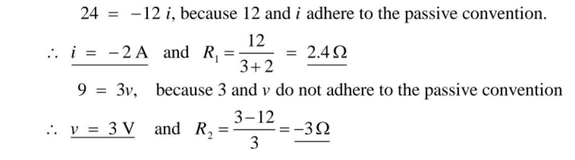
24 12 , because 12 and adhere to the passive convention. 12

2 A and 2.4 3 2

9 3 , because 3 and do not adhere to the passive convention 3 12

3 V and 3 3

i i

i R

v v

v R

 

     

 



     

The situations described in (b) and (c) cannot occur if R1 and R2 are required to be nonnegative.

P 3.2-12 Determine the voltage and current of each of the circuit elements in the circuit shown in Figure P 3.2-12.

Figure P 3.2-12

Solution: We can label the circuit as follows:

The subscripts suggest a numbering of the circuit elements. Apply KCL at node b to get

4 0.25 0.75 0 4 1.0 A

i     i  

Next, apply KCL at node d to get

3 4 0.25 1.0 0.25 0.75 A

Next, apply KVL to the loop consisting of the voltage source and the 60  resistor to get

2 15 0 2 15 V

v    v 

Apply Ohm’s law to each of the resistors to get

2 2

15

0.25 A 60 60

v

i    , v₃10i₃10





 

Next, apply KCL at node c to get

1 2 3 1 3 2 0.75 0.25 1.0 A

i  i i  i    i i   

Next, apply KVL to the loop consisting of the 0.75 A current source and three resistors to get

6 4 3 2 0 6 4 3 2 20 ( 7.5) 15 12.5 V

v v v v   v v v v       

Finally, apply KVL to the loop consisting of the 0.25 A current source and the 20  resistor to get





5 4 0 5 4 20 20 V

v v   v     v 

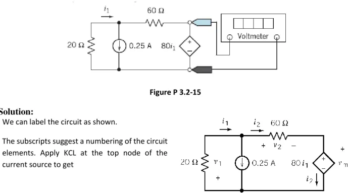
P 3.2-15 Determine the value of the voltage that is measured by the meter in Figure P 3.2-15.

Figure P 3.2-15

Solution:

We can label the circuit as shown.

1 2 0.25

i  i

Apply Ohm’s law to the resistors to get

1 20 1

v  i and v₂ 60i₂ 60









2 1 1 1 1 1 1

15

80 0 60 15 80 20 0 0.09375 A

160

v  i v   i   i  i   i  

Finally, vm 80i1 80 0.09375





P 3.2-17 Determine the current i in Figure P 3.3-17.

Figure P 3.3-17

Solution:

Apply KCL at node a to determine the current in the horizontal resistor as shown.

Apply KVL to the loop consisting of the voltages source and the two resistors to get

-4(2-i) + 4(i) - 24 = 0  i = 4 A

Figure P 3.3-7

Solution:

All the elements are connected in series.

Replace the series voltage sources with a single equivalent voltage having voltage 12 + 12 – 18 = 6 V.

Replace the series 15 , 5  and 20  resistors by a single equivalent resistance of 15 + 5 + 20 = 40 .

By voltage division

10 6

6 1.2 V

10 40 5

v_ _  



 

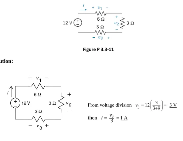
Figure P 3.3-11

Solution:

3

3

3

From voltage division 12 3 V 3 9

= = 1 A 3

then

v

v i

 

 

 

 _ 

P 3.4-8 Determine the value of the voltage v in Figure P 3.4-8.

Figure P 3.4-8

Solution:

Each of the resistors is connected between nodes a and b. The resistors are connected in parallel and the circuit can be redrawn like this:

Then 40 ∥ 20 ∥ 40 = 10Ω

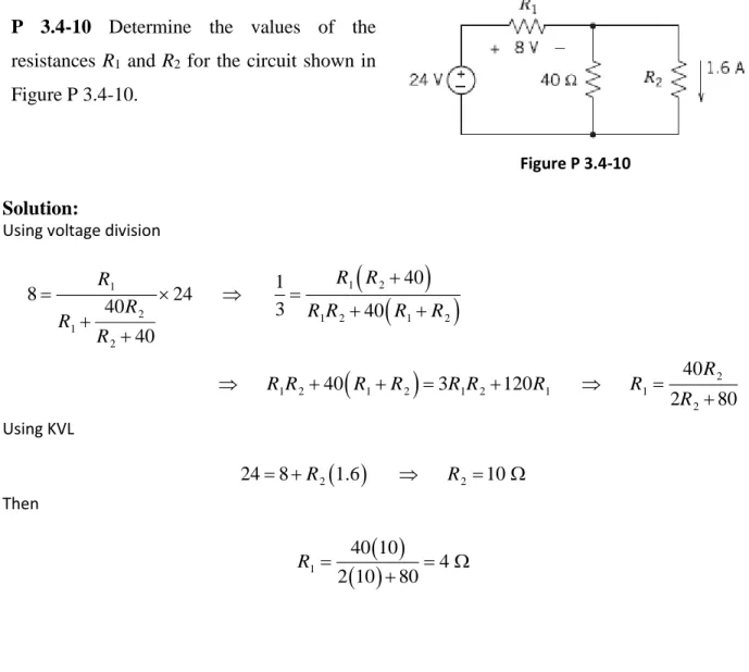
P 3.4-10 Determine the values of the resistances R1 and R2 for the circuit shown in Figure P 3.4-10.

Figure P 3.4-10

Solution:

Using voltage division













1 2

1

2 _{1 2 1 2}

1 2

2

1 2 1 2 1 2 1 1

2 40

1

8 24

40 3 40

40

40

40 3 120

2 80

R R R

R _{R R R R}

R R

R

R R R R R R R R

R                  Using KVL

 

24 8 R 1.6  R 10  Then

 

 

R   



P 3.5-2 Determine the power supplied by each source in the circuit shown in Figure P 3.5-2.

Solution:

The 20- and 5- resistors are connected in parallel. The equivalent resistance is 20 5 4 20 5

 _{ }

 . The

7- resistor is connected in parallel with a short circuit, a 0-7- resistor. The equivalent resistance is 0 7

0 0 7

 _{ }

 , a short circuit.

The voltage sources are connected in series and can be replaced by a single equivalent voltage source.

After doing so, and labeling the resistor currents, we have the circuit shown.

The parallel current sources can be replaced by an equivalent current source.

Apply KVL to get

 

1 1

5 v 4 3.5 0 v 19 V

     

The power supplied by each sources is:

P 3.6-2 The circuit shown in Figure P 3.6-2a has been divided into three parts. In Figure P 3.6-2b, the rightmost part has been replaced with an equivalent circuit. The rest of the circuit has not been changed. The circuit is simplified further in Figure 3.6-2c. Now the middle and rightmost parts have been replaced by a single equivalent resistance. The leftmost part of the circuit is still unchanged.

Figure P 3.6-2

(a) Determine the value of the resistance R1 in Figure P 3.6-2b that makes the circuit in Figure P 3.6-2b equivalent to the circuit in Figure P 3.6-2a.

(b) Determine the value of the resistance R2 in Figure P 3.6-2c that makes the circuit in Figure P 3.6-2c equivalent to the circuit in Figure P 3.6-2b.

(c) Find the current i1 and the voltage v1 shown in Figure P 3.6-2c. Because of the

equivalence, the current i1 and the voltage v1 shown in Figure P 3.6-2b are equal to the current i1 and the voltage v1 shown in Figure P 3.6-2c.

Hint: 24 = 6(i1–2) + i1R2

(d) Find the current i2 and the voltage v2 shown in Figure P 3.6-2b. Because of the

equivalence, the current i2 and the voltage v2 shown in Figure P 3.6-2a are equal to the current i2 and the voltage v2 shown in Figure P 3.6-2b.

Hint: Use current division to calculate i2 from i1.

Solution:

1

2 3 6

( ) 4 6

3 6

1 1 1 1

( ) 2.4 then 8 10.4

12 6 6 p p

p

a R

b R R R

R



   



         

2 1 2 2 1

1 1

1 1 1 2

( ) KCL: 2 and 24 6 0

24 6 ( 2) 10.4 0

36

= =2.195 A = =2.2 (10.4)=22.83 V 16.4

c i i i R i

i i

i v i R

             









3 2 3

1 6

( ) 2.195 0.878 A,

1 1 1

6 6 12

0.878 (6) 5.3 V

6

( ) 0.585 A 3 1.03 W

3 6

d i v

e i i P i

 

 

 

    

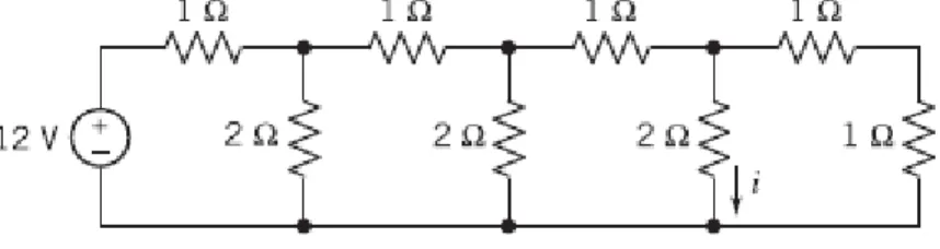
P 3.6-3 Find i using appropriate circuit reductions and the current divider principle for the circuit of Figure P 3.6-3.

Figure P 3.6-3

Solution:

Reduce the circuit from the right side by repeatedly replacing series 1  resistors in parallel with a 2  resistor by the equivalent 1  resistor

This circuit has become small enough to be easily analyzed. The vertical 1  resistor is equivalent to a 2  resistor connected in parallel with series 1  resistor:



  

1

1 1

1.5 0.75 A 2 1 1

i   

P 3.6-21 Determine the value of the resistance R in the circuit shown in Figure P 3.6-22, given that Req = 9 Ω.

Figure P 3.6-22

Solution:

Replace parallel resistors by an equivalent resistor:

8 || 24 = 6 

A short circuit in parallel with a resistor is equivalent to a short circuit.

Replace series resistors by an equivalent resistor: 4+6 = 10 

Now





eq

9R  5 12 ||R||10

So

60 11

4 15

60 11

R

R R



   

P 3.6-28 Determine the value of the resistance R that causes the voltage measured by the voltmeter in the circuit shown in Figure P 3.6-28 to be 6 V.

Figure P 3.6-28

Solution:

Use current division in the top part of the circuit to get

 

a

40

3 2.4 A 40 10

i _ _   



 

Next, denote the voltage measured by the voltmeter as vm and use voltage division in the bottom part of the circuit to get





m a a

5 5

18 18

R R

v i i

R R      _{ }  _{ }      

Combining these equations gives:





When vm = 6 V,

12 6 18

6 18

18 12 6

DP 3-5 The input to the circuit shown in Figure DP 3.5 is the voltage source voltage, vs. The output is the voltage vo. The output is related to the input by

2

o s s

1 2

R

v v gv

R R

 



The output of the voltage divider is proportional to the input. The constant of proportionality, g, is called the gain of the voltage divider and is given by

2 1 2 R g R R  

Figure DP 3.5

The power supplied by the voltage source is

2 2

s s s

s s s

1 2 1 2 in

v v v

p v i v

R R R R R

 

  _{ } 

 

 

where

Rin = R1 + R2 is called the input resistance of the voltage divider. (a) Design a voltage divider to have a gain, g = 0.65.

(b) Design a voltage divider to have a gain, g = 0.65, and an input resistance, Rin = 2500 Ω.

Solution:

Notice that 2 1





1 2

1

R

g g R g R

R R

   



Thus either resistance can be determined from the other resistance and the gain of the voltage divider. Also 2 2 2 in

1 2 in

R R

g R g R

R R R

   



Consequently g R1  













(a) The solution of this problem is not unique. Given any value of R1, we can determine a value of R2 that will cause g= 0.65. Let’s pick a convenient value for R1, say

1 100

R  

Then ₁





g R

g R g R R

g



      

 

P 4.2-2 Determine the node voltages for the circuit of Figure P 4.2-2.

Answer: v1 = 2 V, v2 = 30 V, and v3 = 24 V

Figure P 4.2-2 Solution:

KCL at node 1: 1 2 1 1 0 5 20 1 2 20 5

v v v

v v



      

KCL at node 2: 1 2 2 2 3 3 2 40

1 2 3

20 10

v v v v

v v v

 

      

KCL at node 3: 2 3 1 3 3 5 30

2 3

10 15

v v v

v v



     

P 4.2-6 Simplify the circuit shown in Figure P 4.2-6 by replacing series and parallel resistors with equivalent resistors; then analyze the simplified circuit by writing and solving node equations.

(a) Determine the power supplied by each current source.

(b) Determine the power received by the

12-Ω resistor. Figure P 4.2-6

Solution: Replacing series and parallel resistors with equivalent resistors we get

12Ω + (40Ω ∥ 10Ω) = 20Ω

60Ω ∥ 120Ω = 40Ω

The node equations are





1 2 1 3

3

1 2 3

3 10 0.06 2

20 20

v v v v

v v v

  

      

1 2 2 3

3

1 2 3

2 10 0.04 3 2

20 10

v v v v

v v v

  

       





2 3 1 3 3

1 2 3

0 2 4 7

10 20 40

v v v v v

v v v

 

      

Solving, e.g. using MATLAB, gives

1 1

2 2

3 3

2 1 1 .06 0.244

1 3 2 .04 0.228

2 4 7 0 0.200

(a) The power supplied by the 3 mA current source is









3 10  0.244 = 0.732 mW. The power supplied by the 2 mA source is









2 10  0.228 0.456 mW.

(b) The current in the 12  resistor is equal to the current 1 2 0.244 0.228 0.8 mA

20 20

v v

i     so

the power received by the 12  resistor is





 