Vol. 13, No. 2, pp 209-224
A New Class of Zero-Inflated Logarithmic Series
Distribution
C. Satheesh Kumar, A. Riyaz
Department of Statistics, University of Kerala, Trivandrum, India.
Abstract. Through this paper we suggest an alternative form of the modified zero-inflated logarithmic series distribution of Kumar and Riyaz (Statistica, 2013) and study some of its important aspects. The method of maximum likelihood is employed for estimating the parameters of the distribution and certain test procedures are considered for testing the significance of the additional parameter of the model. Further, all the procedures are illustrated with the help of two real life data sets. Keywords. Generalized likelihood ratio test, logarithmic series distri-bution, maximum likelihood estimation, probability generating function, Rao’s score test.
MSC: 60E05, 60E10.
1
Introduction
The logarithmic series distribution (LSD) and its generalized versions have received much attention in the literature. For example see Khang and Ong (2007), Kumar and Riyaz (2013a) or Johnson et.al. (2005). A limitation of the LSD in certain practical situations is that it ex-cludes zero observation from its support. Khatri (1961) considered a distribution namely ”the logarithmic-with-zeros distribution (LZD)” for modelling such experimental phenomena with excess zero observations.
C. Satheesh Kumar([email protected]), A. Riyaz( )(riyazstatoyour @gmail.com)
Received: November 2013; Accepted: April 2014
Khatri (1961) defined the LZD through the following probability mass function (pmf), in which 0< ω, θ <1.
f1(x) =
{
ω, f or x= 0
(1−ω)θx
−xln(1−θ), x= 1,2, ...
(1.1) Some aspects of the LZD is also available in Johnson et al. (2005, pp.355). Kumar and Riyaz (2013b) considered another zero-inflated log-arithmic series distribution, namely the ”zero-inflated loglog-arithmic series distribution (ZILSD)”, through the following pmf, for x= 0,1,2,· · ·
f2(x) =
Aθx
x+ 1, (1.2)
where A=θ[−ln(1−θ)]−1 and 0 < θ <1. The probability generating function of the ZILSD with pmf (1.2) is
Q1(z) =−Az−1ln(1−θz). (1.3)
Note that ZILSD with pmf (1.2) belongs to the generalized power se-ries family of distributions as well as the Kemp family of distributions, studied by Kumar (2009).
Kumar and Riyaz (2013b) considered a modified form of the ZILSD, namely the ”the modified zero-inflated logarithmic series distribution (MZILSD)”, through the following pgf.
Q2(z) =−Λ(θ1z+θ2z2)−1ln(1−θ1z−θ2z2). (1.4)
where Λ = [−ln(1−θ1 −θ2)]−1(θ1 +θ2), θ1 > 0, θ2 ≥ 0 such that
θ1 +θ2 < 1. Note that the MZILSD with pgf (1.4) reduces to the
pgf (1.3) of the ZILSD when θ2 = 0.
Through this paper we consider the alternative form of the MZILSD and named it as ”the alternative modified zero-inflated logarithmic series distribution (AMZILSD)”, and derive some of its important properties. In section 2 we present the definition of its pgf and derive expression for its pmf, mean and variance. Certain recurrence relations for its proba-bilities, raw moments and factorial moments are also obtained here. In section 3 we discuss the estimation of the parameters of the AMZILSD by the method of maximum likelihood. In section 4 we describe certain test procedures for testing the significance of the additional parameter of the AMZILSD by using generalized likelihood ratio test and Rao’s efficient score test. Both the estimation and testing procedures are il-lustrated with the help of two real life data sets.
2
Definition and Properties
In this section we present the definition and some important properties of the AMZILSD.
Definition 2.1. A non-negative integer valued random variable Y is said to follow ”the alternate modified zero-inflated logarithmic series distribution (AMZILSD)” if its pgf is of the following, in which ∆ = [−ln(1−θ1 −θ2 −α)]−1(θ1 +θ2 +α), θ1 > 0, θ2 ≥ 0, α ≥ −1 and
|θ1+θ2+α|<1 such thatθ1+θ2 ̸=−α.
G(z) = ∆(θ1z+θ2z2+α)−1[−ln(1−θ1z−θ2z2−α)] (2.1)
A distribution with pgf (2.1) we call ”alternate modified zero-inflated logarithmic series distribution” or in short ”AMZILSD”. Clearly, when α= 0 the pgf (2.1) reduces to the pgf of the MZILSD as given in (1.4). The pgf of AMZILSD given in (2.1) can also be written as
G(z) = ∆2F1(1,1; 2;θ1z+θ2z2+α), (2.2)
with
∆−1 =2F1(1,1; 2;θ1+θ+ 2 +α),where
2F1(a, b;c;z) =
∞
∑ r=0
(a)r(b)r (c)r
zr
r! (2.3)
is the Gauss hypergeometric function, in which (d)r =d(d+ 1)· · ·(d+
r−1) forr ≥1 and (d)0 = 1 for anyd∈R= (−∞,∞). For details
re-garding Gauss hypergeometric function see Mathai and Haubold (2008) or Slater (1966).
Now, we obtain the following results in the light of the series repre-sentation:
∞
∑ x=0
∞
∑ r=0
A(r, x) = ∞
∑ x=0
x ∑ r=0
A(r, x−r) (2.4)
and
∞
∑ x=0
∞
∑ r=0
B(r, x) = ∞
∑ x=0
[x
2] ∑ r=0
B(r, x−2r), (2.5)
where [a] denote the integer part of a, for anya≥0.
Result 2.1. For x = 0,1,2, . . ., the pmf g(x) = P(Y = x) of the AMZILSD with pgf (2.1) is the following, in which, βν(α) = 2F1(1 +
ν,1 +ν; 2 +ν;α), f or any ν≥0.
g(x) = ∆
[x2]
∑ r=0
βx−r(α)
(x−r)! (x−r+ 1)
θx1−2r (x−2r)!
θ2r
r! (2.6)
Proof. By the definition of pgf given in (2.1), we have
G(z) = ∞
∑ x=0
g(x)zx (2.7)
= ∆
∞
∑ x=0
(θ1z+θ2z2+α)−1[−ln(1−θ1z−θ2z2−α)]zx.(2.8)
On expanding the logarithmic function in (2.8), to obtain
G(z) = ∆ ∞
∑ x=1
(θ1z+θ2z2+α)x−1
x
= ∆
∞
∑ x=0
(θ1z+θ2z2+α)x
x+ 1
= ∆ ∞ ∑ x=0 x ∑ p=0 ( x p )
(θ1z+θ2z2)x−p
(x+ 1) α p = ∆ α ∑ x=0 x ∑ p=0
x−p ∑ r=0
(
x p
) (x−p r
)
(x+ 1)θ x−p−r
1 θ
r
2αpzx+r−p (2.9)
by binomial theorem. Now by applying (2.4) in (2.9), we get
G(z) = ∆ ∞ ∑ x=0 ∞ ∑ p=0 x ∑ r=0
(x+p p
)(x r )
(x+p+ 1)θ x−r
1 θ
r
2αpzx+r (2.10)
= ∆ ∞ ∑ x=0 ∞ ∑ p=0 ∞ ∑ r=0 (
x+p+r p
) (x+r r
)
(x+p+r+ 1)θ x
1θr2αpzx+2r,(2.11)
by (2.4). By applying (2.5) in (2.11) we obtain
G(z) = ∆ ∞
∑ x=0
∞
∑ p=0
[x2]
∑ r=0
(
x+p−r p
) (x−r r
)
(x+p−r+ 1)θ x−2r
1 θ
r
2αpzx (2.12)
= ∆
∞
∑ x=0
∞
∑ p=0
[x2]
∑ r=0
(x+p−r)!(x−r)! (x−r)!(x+p−r+ 1)
θ1x−2r (x−2r)!
θ2r r!
αp p!z
x,(2.13)
which implies the following, in the light of the relation (1 +ν)p = (ν+ν!p)! and the definition of the generalized hypergeometric function.
G(z) = ∆ ∞
∑ x=0
[x2]
∑ r=0
βx−r(α)
(x−r)! (x−r+ 1)
θx1−2r (x−2r)!
θr2 r!z
x (2.14)
Now on equating the coefficients ofzx on the right hand side expression of (2.7) and (2.14) we get (2.6).
Remark 2.1. Whenα= 0, the pmf of (2.6) of the AMZILSD reduces to the following pmf of the MZILSD, given in (1.4) of Kumar and Riyaz (2013b).
g1(x) = Λ [x2]
∑ r=0
(x−r)! (x−r+ 1)
θx1−2r (x−2r)!
θr2
r!, (2.15)
in which Λ is as given in (1.4).
In order to establish certain recurrence relations for probabilities, raw moments and factorial moments of the AMZILSD, we need the following notations. For i= 0,1,2,· · ·
u+i= (1 +i,1 +i,2 +i), (2.16)
δi=
(1 +i)(1 +i)
(2 +i) , (2.17)
and
∆i=2F1(1 +i,1 +i; 2 +i; θ1+θ2+α) (2.18)
with ∆0= ∆, as defined in (2.2). Here after, we denote the pmfg(x) of
the AMZILSD by g(x;u). In the light of notations (2.16) to (2.18), we can write g(x;u+i) as
g(x;u+i) =eα∆i−1δi
[x2]
∑ r=0
θ1x−2r (x−2r)!
θ2r
r!. (2.19)
proof of (2.19) is given in Appendix A.
Result 2.2. For x ≥ 0, a simple recurrence relation for probabili-ties g(x;u) of the AMZILSD is the following, in which for any positive integer r, g(−r;u) = 0.
(x+ 1)g(x+ 1;u) =δ0∆−01∆1[θ1g(x;u+ 1) + 2θ2g(x−1;u+ 1)](2.20)
Proof. From (2.2) we have
G(z) = ∞
∑ x=0
g(x;u)zx (2.21)
= ∆−012F1(1,1; 2; θ1z+θ2z2+α). (2.22)
Differentiating the right hand side expression of (2.21) and (2.22) with respect toz, we get
∞
∑ x=0
xg(x;u)zx−1 =δ0∆−01(θ1+ 2θ2z)2F1(2,2; 3; θ1z+θ2z2+α).(2.23)
From (2.21) and (2.22) we obtain the following.
∆1
∞
∑ x=0
g(x;u+ 1)zx=2F1(2,2; 3; θ1z+θ2z2+α) (2.24)
By applying (2.24) in (2.23) we have ∞
∑ x=0
xg(x;u)zx−1=δ0∆−01∆1
∞
∑ x=0
(θ1+ 2θ2z)g(x;u+ 1)zx (2.25)
Equating the coefficients ofzx on both sides of (2.25) we obtain (2.20). Result 2.3. Forr≥0, a simple recurrence relation for raw moments
µr(u) of AMZILSD is the following.
µr+1(u) =δ0∆−01∆1
r ∑ j=0
(
r j
)
(θ1+ 2j+1θ2)µr−j(u+ 1) (2.26)
Proof. The characteristic function of the AMZILSD with pgf given in (2.2) has the following representation. Forz∈R andi=√−1,
ϕY(z) =
∞
∑ r=0
µr(u) (iz)r
r! (2.27)
= ∆−012F1(1,1; 2;θ1eiz+θ2e2iz+α). (2.28)
On differentiating the right side expressions of (2.27) and (2.28) with respect toz, we get
∞
∑ r=0
µr(u)
(iz)r−1 (r−1)!
=δ0∆−01(θ1eiz+ 2θ2e2iz)2F1(2,2; 3;θ1eiz+θ2e2iz+α). (2.29)
From (2.27) and (2.28) we also obtain
∆1
∞
∑ r=0
µr(u+ 1) (iz)r
r! =2F1(2,2; 3;θ1e iz +θ
2e2iz+α). (2.30)
Equations (2.29) and (2.30) together implies ∞
∑ r=0
µr(u)
(iz)r−1
(r−1)! = δ0∆ −1 0 ∆1
∞
∑ r=0
(θ1eiz+ 2θ2e2iz)µr(u+ 1) (iz)r
r! = δ0∆−01∆1[θ1
∞ ∑ r=0 ∞ ∑ j=0
µr(u+ 1) (iz)r+j
r!j!
+2θ2
∞ ∑ r=0 ∞ ∑ j=0
µr(u+ 1)
(2iz)r+j r!j! ]
= δ0∆−01∆1[θ1
∞ ∑ r=0 r ∑ j=0
µr−j(u+ 1) (iz)r (r−j)!j!
+2θ2
∞ ∑ r=0 r ∑ j=0
µr−j(u+ 1)
(2iz)r
(r−j)!j!] (2.31) by (2.4). Now, on equating the coefficients of (r!)−1(iz)r on both sides of (2.31) we get (2.26).
Result 2.4. For r ≥ 1, a simple recurrence relation for factorial momentsµ[r](u) of the AMZILSD is the following, in whichµ[0](u) = 1.
µ[r+1](u) =δ0∆−01∆1[(θ1+ 2θ2)µ[r](u+ 1) + 2θ2rµ[r−1](u+ 1)] (2.32)
Proof. From (2.2) we have the following factorial moment generating functionF(z) of the AMZILSD
F(z) = ∞
∑ r=0
µ[r](u)
zr
r! (2.33)
= ∆−012F1[1,1; 2;θ1(1 +z) +θ2(1 +z)2+α]. (2.34)
On differentiating the right hand side expressions of (2.33) and (2.34) with respect toz, we get
∞
∑ r=0
µ[r](u)
zr−1 (r−1)!
=δ0∆−01[θ1+θ2(1 +z)]2F1[2,2; 3;θ1(1 +z) +θ2(1 +z)2+α].(2.35)
From (2.33) and (2.34) we have
∆1
∞
∑ r=0
µ[r](u+ 1)
zr
r! =2F1[2,2; 3;θ1(1 +z) +θ2(1 +z)
2+α]. (2.36)
Equations (2.33) and (2.34) together implies the following. ∞
∑ r=0
µ[r](u)
zr−1
(r−1)! =δ0∆ −1 0 ∆1
∞
∑ r=0
[θ1+ 2θ2(1 +z)]µ[r](u+ 1)
zr r!(2.37)
On equating the coefficients of (r!)−1zr on both sides of (2.37) we get (2.32).
By using the Result 2.4, we obtain the mean and variance of the AMZILSD, as given in the following result.
Result 2.5. The mean and variance of the AMZILSD are given below.
E(Y) = δ0∆0−1∆1(θ1+ 2θ2)
V ar(Y) = δ0∆−02(δ1∆0∆2−δ0∆12)(θ1+ 2θ2) +δ0∆0−1∆1(θ1+ 2θ2).
Proof is simple and hence omitted.
3
Estimation
In this section we discuss the estimation of the parameters θ1,θ2 and α
of the AMZILSD by the method of maximum likelihood and illustrate the procedures using certain real life data sets.
Leta(x) be the observed frequency ofxevents and let y be the highest value of x. Then the likelihood function of the sample is
L= y ∏ x=0
[g(x)]a(x), (3.1)
where g(x) is the pmf of the AMZILSD as given in (2.6). Now taking logarithm on both sides of (3.1), we have
logL = y ∑ x=0
a(x) log[g(x)]
= y ∑ x=0
a(x)[log ∆ + log Ψ(x;θ1, θ2, α)], (3.2)
where ∆ is as given in (2.1) and
Ψ(x;θ1, θ2, α) = [x2]
∑ r=0
βx−r(α)
(x−r)! (x−r+ 1)
θx1−2r (x−2r)!
θr2 r!.
Let ˆθ1, ˆθ2 and ˆα denote the maximum likelihood estimators of the
AMZILSD respectively. On differentiating(3.2) partially with respect to the parameters θ1,θ2 and α and equating to zero, we get the
follow-ing likelihood equations, in which
D= (θ1+θ2+α)−1−[−ln(1−θ1−θ2−α)]−1(1−θ1−θ2−α)−1.
y ∑ x=0
a(x)
D+
∑[x2]
r=0βx−r(α)(x(x−−rr+1))!
θx1−2r−1
(x−2r−1)!
θr
2 r!
Ψ(x;θ1, θ2, α)
= 0 (3.3)
y ∑ x=0
a(x)
D+
∑[x
2]
r=0βx−r(α)(x(x−−rr+1))! θ
x−2r
1
(x−2r)!
θr2−1
(r−1)!
Ψ(x;θ1, θ2, α)
= 0 (3.4)
and y ∑ x=0
a(x)
D+
∑[x2]
r=0βx−r+1(α)((xx−−rr+1)!+2)
θ1x−2r
(x−2r)!
θr2 r!
Ψ(x;θ1, θ2, α)
= 0. (3.5)
When likelihood equations do not have a solution, the maximum of the likelihood function attained at the border of the domain of the parameters. So we obtained the second order partial derivatives of log[g(x)] with respect to the parameters θ1,θ2 and α by using
MATH-CAD software observed that these eqations give negative values for all θ1 > 0, θ1 ≥ 0, α ≥ −1 and |θ1 +θ2+α| < 1 such thatθ1+θ2 ̸= α.
Thus the density of the AMZILSD is log-concave and hence the maxi-mum likelihood estimators of the parametersθ1,θ2andαare unique (cf.
Puig, 2007). Now, on solving these likelihood equations (3.3), (3.4) and (3.5) by using some mathematical software such asMATHLAB,
MATH-CAD, MATHEMATICA etc., one can obtain the maximum likelihood
estimators of the parameters θ1,θ2 and α of the AMZILSD.
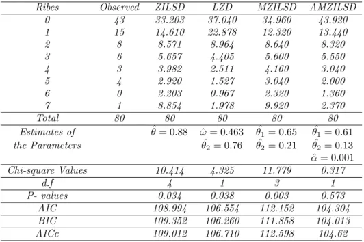
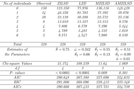
For numerical illustration, we have considered two real life data sets of which the first data is on Ribes, Kaniksu, Idaho taken from Fracker and Brischle (1944) and the second data set on Juncuss effuses seed-ings taken from Evans (1953). We have fitted the ZILSD, the LZD, the MZILSD and the AMZILSD to these two data sets and the results ob-tained along with the corresponding values of the expected frequencies, Chi-square statistic, degrees of freedom (d.f), P, Akaike information cri-terion (AIC), Bayesian information cricri-terion (BIC) and the second order Akaike information criterion (AICc) in respect of each of the models are presented in Tables 1 and 2. Based on the computed values of Chi-square statistic, P, AIC, BIC and AICc, it can be observed that the AMZILSD give the best fit to both the data sets where the existing models - the ZILSD, the LZD and the MZILSD fails.
Table 1. Observed frequencies and computed values of expected fre-quencies of the ZLSD, the LZD, the MZILSD and the AMZILAD by the method of moments and the method of maximum likelihood for the first data set.
Ribes Observed ZILSD LZD MZILSD AMZILSD 0 43 33.203 37.040 34.960 43.920 1 15 14.610 22.878 12.320 13.440 2 8 8.571 8.964 8.640 8.320 3 6 5.657 4.405 5.600 5.550 4 3 3.982 2.511 4.160 3.040 5 4 2.920 1.527 3.040 2.000 6 0 2.203 0.967 2.320 1.360 7 1 8.854 1.978 9.920 2.370
Total 80 80 80 80 80
Estimates of θˆ= 0.88 ωˆ = 0.463 θˆ1= 0.65 θˆ1= 0.61
the Parameters θˆ2= 0.76 θˆ2= 0.21 θˆ2= 0.13
ˆ
α= 0.001 Chi-square Values 10.414 4.325 11.779 0.317
d.f 4 1 3 1
P- values 0.034 0.038 0.003 0.573 AIC 108.994 106.554 112.152 104.304 BIC 109.352 106.260 111.858 104.013 AICc 109.012 106.710 112.598 104.62
Table 2. Observed frequencies and computed values of expected fre-quencies of the ZLSD, the LZD, the MZILSD and the AMZILAD by the method of maximum likelihood for the second data set.
No.of individuals Observed ZILSD LZD MZILSD AMZILSD 0 150 123.350 77.976 136.116 148.428 1 34 46.256 91.782 37.392 38.076 2 28 23.128 30.288 22.572 25.136 3 8 13.010 13.327 12.312 9.576 4 4 7.806 6.579 7.296 5.244 5 2 4.789 3.483 4.332 1.010 6 2 9.571 4.547 7.980 0.530
Total 228 228 228 228 228
Estimates of θˆ= 0.75 ωˆ= 0.342 θˆ1= 0.55 θˆ1= 0.51
the Parameters θˆ2= 0.66 θˆ2= 0.13 θˆ2= 0.09
ˆ α= 0.01 Chi-square Values 21.374 108.239 11.64 1.069
d.f 4 3 3 1
P- values <0.0001 <0.0001 0.009 0.301 AIC 290.648 267.380 227.696 224.632 BIC 291.006 268.096 228.412 225.346 AICc 290.666 267.433 227.751 224.739
4
Testing of the Hypothesis
In this section we discuss the testing of hypothesis H0 :α = 0 against
the alternative hypothesis H1 : α ̸= 0 by using generalized likelihood
ratio test and Rao’s efficient score test.
In case of generalized likelihood ratio test, the test statistic is −2 logλ= 2[logL( ˆΩ;x)−logL( ˆΩ∗;x)], (4.1)
where ˆΩ is the maximum likelihood estimator of Ω = (θ1, θ2, α) with no
restrictions, and ˆΩ∗ is the maximum likelihood estimator of Ω whenα = 0. The test statistic−2 logλgiven in (4.1) is asymptotically distributed as Chi-square with one degree of freedom. For details see Rao, (1973). We have computed the values of logL( ˆΩ;x), logL( ˆΩ∗;x) and the test statistic for the AMZILSD for these two data sets and presented in Table 3.
Table 3 : The computed the values oflogL( ˆΩ;x),logL( ˆΩ∗;x) and the generalized likelihood ratio test under H0.
logL( ˆΩ∗;x) logL( ˆΩ;x) Test statistic Data set 1 -54.020 -50.628 6.784 Data set 2 -111.846 109.609 4.654 In case of Rao’s Score test, the statistic is,
S =T′φ−1T, (4.2)
whereT′=
(
1
√
n ∂logL
∂θ1 ,
1
√
n ∂logL
∂θ2 ,
1
√
n ∂logL
∂α )
andφis the Fisher informa-tion matrix. The test statistic given in (4.2) follows Chi-square distri-bution with one degree of freedom, (see Rao, 1973). We have computed the values ofS for the AMZILSD in the case of first data set asS1 and
for the the AMZILSD in the case second data set asS2 as given below.
S1= (
2.902 7.399 −1.522)
−00.101.106 −00.240.106 −00.013.157 0.013 −0.157 0.169
27..902399
−1.522
= 13.231
S2= (
8.75 16.94 −0.959)
−00..0260002 −00.0059.0002 −−00..0066033
−0.033 −0.0066 0.057
168.75.94
−0.959
= 4.447
Since the critical value for the test at 5% level of significance and one degree of freedom is 3.84, the null hypothesis is rejected in all the above cases in respect of generalized likelihood ratio test and Rao’s efficient score test.
5
Appendix - A
Proof of Equation(2.19). From (2.7) we have the following, in the light of (2.16) and (2.18).
G(z) = ∞
∑ x=0
g(x;u+i)zx (5.1)
= ∆−i 12F1(1 +i,1 +i; 2 +i;θ1z+θ2z2+α). (5.2)
On expanding the Gauss hypergeometric function in (5.2), we obtain
G(z) = ∆−i 1 ∞
∑ x=0
(1 +i)x(1 +i)x (2 +i)x
(θ1z+θ2z2+α)
x! (5.3)
= ∆−i 1 ∞
∑ x=0
(1 +i)x(1 +i)x (2 +i)x
x ∑ p=0 ( x p )
(θ1z+θ2z2)x−p
x! α
p
= ∆−i 1 ∞
∑ x=0
(1 +i)x(1 +i)x (2 +i)x ×
x ∑ p=0
x−p ∑ r=0
(
x p
)(x−p r
)
x! θ x−p−r
1 θ
r
2αpzx+r−p (5.4)
by binomial theorem. Apply (2.4) in (5.4) to get
G(z) = ∆−i 1 ∞
∑ x=0
(1 +i)x(1 +i)x (2 +i)x
∞ ∑ p=0 x ∑ r=0
(x+p p
)(x r )
(x+p)!θ x−r
1 θ2rαpzx+r (5.5)
= ∆−i 1 ∞
∑ x=0
(1 +i)x(1 +i)x (2 +i)x
× ∑∞ p=0 x ∑ r=0 (
x+p+r p
) (x+r r
)
(x+p+r)!θ x
1θr2αpzx+2r, (5.6)
by applying (2.4) again. Now, by using (2.5), we have the following from (5.6).
G(z) = ∆−i 1 ∞
∑ x=0
(1 +i)x(1 +i)x (2 +i)x
× ∑∞
p=0 [x2]
∑ r=0
(
x+p−r p
) (x−r r
)
(x+p−r)!θ x−2r
1 θ2rαpzx (5.7)
= eα∆−i 1 ∞
∑ x=0
(1 +i)x(1 +i)x (2 +i)x
[x
2] ∑ r=0
θ1x−2r (x−2r)!
θ2r r!z
x. (5.8)
On equating the coefficients of zx on the right hand side expressions of (5.1) and (5.8), we get (2.19).
Acknowledgements
The authors grateful to the Editor, Associate Editor and anonymous referees for their valuable comments on an earlier version of the paper.
References
Evans, D. A.(1953), Experimental evidence concerning contagious dis-tributions in ecology. Biometrika, 40, 186-211.
Fracker, D. B. and Brischle, H. A.(1944), Measuring the local distribu-tion of Ribes. Ecology, 25, 253-303.
Johnson, N. L., Kemp, A. W., and Kotz, S.(2005), Univariate Discrete Distributions. New York: Wiley.
Khang, T. F. and Ong, S. H.(2007), A new generalization of the loga-rithmic distribution arising from the inverse trinomial distribution. Communications in Statistics-Theory and Methods, 36, 3-21. Khatri, C. G. (1961), On the distribution obtained by varying the
num-ber of trials in a binomial distribution. Annals of the Institute of Statistical Mathematics, 13, 47-51.
Kumar, C. S.(2009), Some properties of Kemp family of distribution. Statistica,69, 311-316.
Kumar, C. S. and Riyaz, A. (2013a), A modified version of logarith-mic series distribution and its applications. Communications in Statistics-Theory and Methods (accepted for publication).
Kumar, C. S. and Riyaz, A. (2013b), On the zero-inflated logarithmic series distribution and its modification. Statistica,73, 477-492. Mathai, A. M. and Haubold, H. J. (2008), Special Functions for Applied
Scientists. New York: Springer.
Puig, P. (2003), Characterizing additively closed discrete models by a property of their MLEs with an application to generalized Hermite distribution. Journal of American Statistical Association,98, 687-692.
Rao, C. R. (1973), Linear Statistical Inference and Its Applications. New York: John Wiley.
Slater, L. J. (1966), Generalized Hypergeometric Functions. Cam-bridge: Cambridge University Press.