Math 179: Graph Theory

Evan Chen May 17, 2015

Notes for the course M179: Introduction to Graph Theory, instructed by Wasin So.

1 January 23, 2013

Website: _{www.math.sjsu.edu/~so} contains most of the information. Three handouts: syllabus, calendar, homework

Textbook: A First Course in Graph Theory. “The reason I choose this book is because it’s cheap. All the graph theory books are isomorphic.” We will cover ten chapters.

The grade will consist of:

Homework (20%) 10 assignments. Each chapter will have its own homework; 5 problems for each chapter. Solutions will be posted afterwards. Two assignments will be dropped.

Project (10%) Paired.

Test (30%) Two tests, 15% each. Already on calendar.

Final (40%) Final exam. Wednesday, May 15, 2013, 2:45 PM.

The usual scale applies. However A≥90%,A+≥94% andA− ≥87%. 1.2 Introductory Question

Problem. Which letters can be drawn without lifting the pencil or double tracing? BCDLMNOPQRSUVWZ, notAEFGHIJKLTXY. Yeah this is just Eulerian tours, okay. Problem. Four color theorem on CA map.

Three colors is not sufficient if there is an odd cycle whose vertices are all connected to some other vertex.

Problem. Instant insanity.

Solution. What matters is the opposite color.

R B G Y 1 2 3 3 4 1 3 2 4 4 1 2

Figure 1: Instant Insanity

We need only find four cycles whose edges each have 1,2,3,4, which are disjoint; they are colored in the above diagram. This corresponds to a solution.

1.3 Definitions

Definition. A graphG is a set of verticesV along with a set of edgesE. All three problems can be abstracted into graphs as described.

2 January 28, 2012

ˆ graph

ˆ subgraph

ˆ Walk, trail, path

ˆ Closed walk, circuit, cycle

ˆ Connected graph

ˆ Disconnected graph 2.2 Preliminary Definitions

Definition. A (simple) graphG is an ordered pair (V, E), whereV is a nonempty set, andE is a collection of 2-subsets of V. V is sometimes call deth vertex set ofG , andE

is called the edge set ofG.

Example. LetV ={1,2,3}and E ={{1,2},{1,3}}. This gives a graphG1. Example. LetV ={1,2,3}and E ={{1,2},{2,3}}. This gives a graphG2. Remark. SuchG is called a labelled graph.

2.3 Isomorphism

For human beings, this is not very nice. So, we visualize a graph as a picture. These

1 2 3 Figure 2:G1 1 2 3 Figure 3:G2

two graphs are different, since their edges are different. But if we eliminate the labelling (i.e. we take the unlabelled graph) then these graphs are not the same. In other words,

these graphs areisomorphic.

We want to study graphs, structurally, without looking at the labelling. That is, the more interesting properties of a graph do not rely on the labelling. But labels are useful for implementation, or if we want to introduce some sort of asymmetry.

Definition. The order of a graph Gis |V|. Thesize of Gis |E|.

Definition. Atrivial graph is a graph with order 1. Anempty graph is a graph of size 0. Note that a graph must have at least one vertex by definition. But a graph can certainly have no edges!

For now we are not permitting loops, so trivial graphs are necessarily empty. 2.4 Subgraph

Definition. LetGbe a graph. H is a subgraph ofGifV(H)⊆V(G) andE(H)⊆E(G). Example. LetG3 be the graph with V ={1,2,3}and E={{1,2},{2,3},{3,1}} Then

G1, G2 are subgraphs ofG3 butG1 is not a subgraph of G2. The subgraph isproper if either of these inclusions is strict.

This is a fairly strong condition, but here are some other conditions. Definition. H is aspanning subgraph ifV(H) =V(G).

Example. G1 is a spanning subgraph ofG3. Most important definition:

Definition. H is aninduced subgraph ifuv ∈E(H) ⇐⇒ uv ∈E(G)∀u, v∈V(H).

1 2 3 4 1 2 4 1 2 3 4

In the above figures, the second but not the third graph is an induced subgraph of the first.

2.5 Walks

Definition. Au−vwalk in a graphGis a finite sequence of vertices (u=v0, v1,· · ·, vk =

v) such that vi and vi+1 are adjacent for each 0≤i≤k−1.

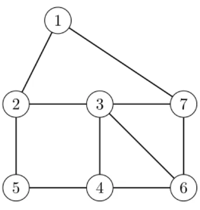
1

5 4 6

2 3 7

Figure 4: Yet another graph

ˆ (1,2,3,4,5,2,3,7)

ˆ (1,7)

ˆ (1,2,3,7)

ˆ (1,2,3,6,4,3,7)

ˆ (1,7,1,7)

Note that (1,7,7) is not a walk since {7,7} is not an edge. Also, (1,7,1) is a (1,1) walk. Definition. A walk is closed if and only if u=v. Otherwise, it is open.

Definition. A trail is an open walk without repeating vertices. Definition. A path is an open walk without repeating vertices.

Note that paths are trails, but not vice-versa.

Definition. A circuit is a closed walk without repeating edges.

Definition. A cycle is a closed walk without repeating vertices, other than the initial and terminal vertices.

Theorem 2.1 (Chartrand and Zhang, 1.6). If there is au−v walk between two vertices, then there is also au−v path.

Proof. Take the minimal walk. If it’s not a path trim it, contradiction. 2.6 Connectedness

Definition. A graphG isconnected if∀u, v∈V(G) there exists a u−v path.

Definition. Let G be a connected graph. Then d(u, v) is the smallest length of any

u−v path ifu6=v, or 0 if u=v. Example. In figure 4, d(1,2) = 1 d(1,3) = 2 d(1,4) = 3 d(1,5) = 2 d(1,6) = 2 d(1,7) = 1 1 2 3 4 5 6

Figure 5: A cycle graph

Definition. The diameter of a connected graph Gis defined as

G= max

u6=v d(u, v). Example. The diameter of 4 is 3.

Remark. By construction,d(u, v)≤diam(G)∀u, v∈V(G).

Remark. The six degrees of separation suggests that diam(G)≈6, whereV is the set of people, andE represents acquaintance.

How do we check if a graph is connected?

Theorem 2.2 (Chartrand and Zhang, 1.10). IfordG≥3 then G is connected if and only if there exist verticesu6=v in Gsuch that G−u and G−v are both connected. Proof. First we prove the condition is sufficient. We wish to show xand y are connected for any x, y ∈ V(G). If {x, y} 6= {u, v} it’s trivial; otherwise, take some vertex w not equal to either {u, v} and walk fromu tow thenv. This is possible since ordG≥3.

For the converse, consider a connected graph G. Pick a diameteru−v ofG. We claim this works. Assume on the contrary that G−u is not connected. Then ∃x, y ∈V(G) such that all x−y paths contain u. Now consider v. If x andv are not connected in

G−u thenx−u−v is longer than u−v. Sox and v are connected. Similarlyy andv

are connected. So x andy are connected. To wrap up:

Definition. A graph is disconnected if it is not connected.

So we can measure the disconnected-ness by looking atconnected components. Definition. Given a graph G, then we define ∼by u∼v when there is a u−v path. Then ∼is an equivalence relationship, and its classes are the connected components.

3 January 30, 2013

Reminder: homework due next Monday. 3.1 Today’s Topics

ˆ Graph classes

ˆ Graph operators

Last time we learned about

ˆ connected graph (diameters)

ˆ disconnected graphs (number of components) 3.2 Classes of graphs

Here are some “prototypcial” graphs.

Empty graph We letEn denote the empty graph with order nand size 0. This graph is disconnected if and only ifn≥2.

Path graph We letPnbe the graph of order nand sizen−1. You can guess what this is: It is connected with diametern−1.

1 2 3 4 5

Figure 6: The graph P5

Cycle graph We let Cn denote the graph of ordern and sizenwhich consists of a single cycle. Note that n≥3. It is connected with diameter1₂n.

1 2 3

4

5

Figure 7: The graph C5

Complete Graph We letKn denote the complete graph, with orderr and size n₂

. It is extremely connected with diameter 1 (forn≥2). Note that this is the only class of connected graphs with diameter 1.

3.3 Bipartite Graphs Some more general graphs:

Bipartite graph A graph Gis bipartite ifV(G) =UtV for some nonemptyU, V such that if u1u2, v1v2 ∈/ V(G) foru,u2 ∈ U, v1, v2 ∈G. In other words, the induced subgraphsG[U] andG[W] are completely disconnected. In still other words,Ghas chromatic number at most 2 and|V(G)| ≥2.

For example,En is trivially bipartite for n≥2. Similarly,Pn is bipartite if n≥2. (In fact, all trees are bipartite.) More interestingly,Cn is bipartite if and only ifn

is even. And of course,Kn isn’t bipartite unlessn= 2.

Complete bipartite graph For integers s, t the graph Ks,t is a bipartite graph with s vertices of one color and tvertices of the other color, and any two vertices of the opposite colors are joined. The order is s+t and size is st. The diameter is at most 2.

Theorem 3.1 (Chartrand and Zhang, 1.12). A graphG is bipartite if and only ifG has no odd cycle.

Proof. If there is an odd cycle we clearly lose (just take a cycleC = (c0, c1,· · · , c2k+1) with c2k+1 =c0). Color chase.

To show the condition is sufficient, split into connected components. Fix a vertex v0. Then color a vertex v red iff d(v0, v) is even and blue otherwise. In particular, v0 is red. This works as follows: consider the paths from v0 to u andv, whereu, v are the same color. Take a vertexk on these paths (possibly equal tov0) for which the geodesics from

ktou and k tov are disjoint. This is clearly possible.

v0

k

u v

Figure 8: Long paths

In general it is pretty hard to show that there are no odd cycles. 3.4 Graph Operations

Graph complement Given G= (V, E), the complement ¯G is defined byV( ¯G) =V(G) and E( ¯G) ={uv :uv /∈E(G)}.

For example, the following two graphs are complements:

a b c d a b c d

Note that if ¯En=Kn. It is not necessarily easy to tell if the complement of a connected graph is connected, but we have a homework problem

Theorem 3.2 (Chartrand and Zhang, 1.11). If G is disconnected, then G¯ is connected anddiam(G)≤2.

Finally, note, of course thatG=G.

Graph union Given G and H with disjoint vertex sets, the graph union ofG and H, denotedG∪H, is defined byV(G∪H) =V(G)∪V(H) andE(G∪H) =E(G)∪E(H). Note thatk(G∪H) =k(G) +k(H). (Here k(G) is the number of components.)

Graph joint Given G and H with disjoint vertex sets, then the graph joint, denoted

G+H, is defined by

V(G+H) =V(G)∪V(H)

E(G+H) =E(G)∪E(H)∪ {uv:u∈V(G), v ∈v(H)} For example,Ks,t=Es+Eh and ¯Ks,t =Ks∪Kt.

In general,G+H = ¯G∪H¯, orG+H = ¯G∪H¯. So a joint is always disconnected (by, say, Chartrand and Zhang, 1.11).

Graph product Given Gand H with disjoint vertex sets, the graph productG×H is defined by: V(G×H) =V(G)×V(H) E(G×H) ={(u, x)(v, x)|uv∈V(G)} ∪ {(x, u)(x, v)|uv ∈V(H)} 1a 2a 1b 2b

Figure 9: K2×K2, with vertex sets {1,2} and {a, b}

1c 1d 1a 1b 2a 2b 2c 2d Figure 10:K2×C4 Note that (G1∪G2)×H= (G1×H)∪G−2×H).

The hypercube can be realized asQn=K2×K2× · · · ×K2

| {z }

ntimes

4 February 4, 2013

ˆ degree

ˆ First Theorem of Graph Theory

ˆ high degree =⇒ connectedness

ˆ regular graph

4.2 The Degree of a Vertex

This is a local parameter because it is defined with respect to a single vertex.

Definition. Given a graphGandv∈V(G),uis said to be aneighbor ofvifuv ∈E(G). The set of all neighbors is called the neighborhood of v, denoted N(v).

Definition. Thedegree of a vertex v, denoted degv or d(v), is the cardinality of the neighborhood ofv.

Some special names.

Definition. We sayv is an isolated vertex if degv= 0. We say it is anend vertex (or leaf) if degv= 1.

Definition. Let δ(G) = minv∈V(G)degv denote the minimum degree. Let ∆(G) = max_v∈V(G)degv denote the maximum degree.

Trivially, 0≤δ(G)≤degv≤δ(G)≤n−1. 4.3 Sum of degrees

Theorem 4.1 (First Theorem in Graph Theory, Chartrand and Zhang, 2.1). For any graphG,

X

v∈V(G)

degv= 2|E(G)|.

Proof. Clear.

Corollary 4.2. The number of vertices of odd degree is even.

Example. Let G be a graph with 14 vertices and 27 edges. Moreover, the number of vertices of degree 3 isx and the number of vertices of degree 4 is 6, and the number of vertices of degree 5 isz. Findx and z.

Solution. We have thatx+ 6 +z= 14 and 3x+ 4·6 + 5z= 2·27. Solving,x= 5 and

z= 3.

Now, can we construct a graph with said degrees? On Wednesday we will find conditions for which there exists a graph with a certain multiset of degrees.

Example. In any graph, there exist two vertices have the same degree.

Occasionally, if degv=|V(G)| −1, then sometimes we call v a universal vertex. How many edges do we need to guarantee a connected graph on nvertices? Answer. n−₂1

+ 1. Consider Kn−1.

This is weak, though. So here is a better criterion.

Theorem 4.3 (Chartrand and Zhang, , 2.4). If degu+ degv≥n−1for all u, v∈V(G), thenG is connected. Moreover, diamG≤2.

Proof. If u andv are disconnected, then look at the neighborhoods ofu and v. They must overlap, since G− {u, v} has justn−2 vertices but|N(u)|+|N(v)|=n−1. This forms a path of length 2.

Random thought: in terms ofn, find the bestk such that if degu+ degv+ degw≥

k∀u, v, w∈V(G), then Gis connected. 4.4 Regular Graph

Definition. A graph is k-regular if degv=k for all v∈V(G).

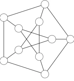
For example, En is 0-regular, and Kn is (n−1)-regular. Furthermore, Ck is 2-regular. A special 3-regular graph is the Peterson graph.

Figure 11: The troll face.

Definition. Givenn and 0≤r ≤n−1 wherern is even, defineHr,n theHarary graph to be anr-regular graph onnvertices, as follows: label the vertices 0,1,· · ·, n−1 modulo

n, and

ˆ Ifr is even, then join each vertexktok−₂1r tok+1₂r (excluding self).

ˆ Ifr is odd, then join each vertex kto k−1₂(r−1) tok+ 1₂(r−1), then tok+ 1₂n. Exercise. Is the Petersen graph a Harary graph?

Theorem 4.4 (Existence Theorem for Regular Graph, Chartrand and Zhang, 2.6).

Given 0≤r ≤n−1, there exists an r-regular graph on n vertices if and only if rn is even.

Proof. To construct an example, use the Harary graph. If rnis odd then apply the First Theorem directly to yield a contradiction.

Figure 12:H2,5,H3,6, and H4,7

4.5 Subgraphs of Regular Graphs

Clearly, every graph of order n is a subgraph of Kn. The question “is every graph of order nan induced subgraph ofKN?” is also no. But now, consider the question:

Is every graph of order nan induced subgraph of some regular graph? Answer: yes.

Example. Pnis an induced subgraph of Cn+1.

Theorem 4.5 (Chartrand and Zhang, 2.7). G is always an induced subgraph of a

∆(G)-regular graph H.

Proof. We perform induction on n= ∆(G)−δ(G). The base casen= 0 is already clear. Make a copy of G, call it G0. Then join all the vertices of minimal degree to each other from GtoG0. This decreasesn by one, so we are done by induction.

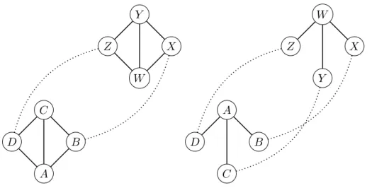
A B C D W X Y Z C B A D Y X W Z

Figure 13: Duplicating graphs G. This drops n = 1 to n = 0 and n = 2 to n = 1, respectively.

5 February 6, 2013

OOPS darn I keep forgetting graphs are loopless. (Also I should read the question.) For 1.17 one can use the following lemma:

Lemma. If nonemptyU, W ⊆V(G)have an empty intersection, then there existsp0 ∈U,

pk∈W, and a pathp0−p1− · · · −pk−1−pk for whichpi ∈/U∪V for each1≤i≤k−1.

Proof. Pick the shortest such path.

For 1.18, the graph with all twelve vertices is actually pretty nice:

Figure 14: All of 1.18

A few remarks about 1.22: the graphG×K2 is called aG-prism. 5.2 Today’s Topics

Chapter 2:

ˆ Degree sequence

ˆ Graphical integer sequence

ˆ Hakimi-Harvel Theorem 5.3 Degree Sequences

Definition. The degree sequence of a graphGis the sequence of degrees of G, arranged in nonincreasing order.

Example. The degree sequence ofP4 is (2,2,1,1).

The degree sequence ofC6 is (2,2,2,2,2,2). So isC3∪C3. The degree sequence ofK4 is (3,3,3,3).

Definition. Given a nonincreasing sequencesof nonnegative integers, we call itgraphical

if there is a graph whose degree sequence is s.

What are some necessary conditions for a graphical sequence of length n? If the sequence isd1≥d2 ≥ · · · ≥dn, then

(ii) 0≤di ≤n−1 for eachi. (iii) d2, d3,· · · , dd1+1 are all nonzero.

(iv) If di =n−1 then dn≥i. (v) If dj = 0 thend1 ≤j−2.

Example. (3,3,3,1) is not graphical. Note thatd3 =n−1 (heren= 4) which would force d4 ≥3, which is false. For similar reasons, (7,7,4,3,3,3,2,1).

OK, we can make more necessary conditions. What are the sufficient conditions? (i) If di =r for alli= 1,2,· · ·, n such thatrnis even, then such a graph exists. (ii) If d1 ≥ d2 ≥ · · · ≥ dn is graphical, then n−1−dn ≥ n−1−d1 is graphical.

(Complement everything). 5.4 Hakami-Havel

Theorem 5.1 (Hakimi-Havel Theorem). A sequence d1≥d2 ≥ · · · ≥dn is graphical if

and only if

d2−1, d3−1,· · ·, dd1+1−1, dd1+2,· · ·, dn

is graphical.

Example. Is 3,3,2,2,1,1 graphical?

Solution. Descending, we get 2,1,1,1,1, then 1,1,0,0 which is graphical, so the answer is yes. We can easily build upwards, to.

Figure 15: 3,3,2,2,1,1 Let us wrap up our example from last time as well.

Example. Is the sequence (di)14i=1= (5,5,5,4,4,4,4,4,4,3,3,3,3,3) graphical?

Solution. Use the Hakimi-Havel Theorem twice to get (d00_i)12_i=1 = (3,3,· · · ,3) which is clearly doable.

Proof of Hakimi-Havel. The sufficient part is easy; just construct it by adding an nth vertex and connecting it to the right vertices.

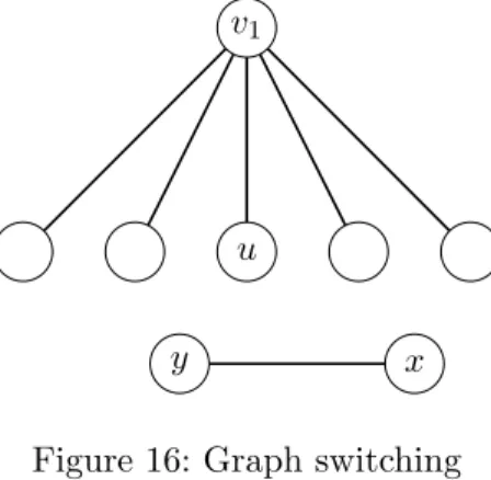
For the necessary part, we claim that there exists a graph Gwith degreed1 ≥ · · · ≥dn such that the neighbors of v1 arev2, v3,· · ·, vd1+1, where degvi=di for each i. Assume

the contrary. PickG with the property that X

v∈N(v1)

u v1

y x

Figure 16: Graph switching

is maximal.

Evidently there exist verticesu∈N(v1) andy /∈N(v1) for which degy >degu. Hence, due to degrees, there is some vertexx∈N(y) such that x /∈N(u). Then delete the edges

uv,xy and add the edges uxand vy. This maintains the degree sequence but increases the sum, contradiction.

6 February 11, 2013

ˆ Isomorphic graphs. 6.2 Isomorphism

Definition. Two graphs Gand H areisomorphic if and only if there exists a biejction

f :V(G)→V(H) such that uv∈E(G) ⇐⇒ f(u)f(v)∈E(H). Such anF is called an

isomorphism.

As an example, the following two graphs are isomorphic:

1 2 3 4 1 2 3 4

Figure 17: Two isomorphic graphs. A bijection is f = (4 3)∈S4. Musing: how many such f exist?

8 6 9 7 10 1 5 4 3 2 7 6 5 10 9 8 1 2 4 3

Figure 18: Petersen again! This thing

6.3 Disproving isomorphism

Graph isomorphism is NP. In other words, it’s pretty hard. Of course, some trivial optimizations; isomorphism preserves:

ˆ the multiset of degrees (in particular, the order and sizes)

ˆ number of connected components (in particular, connectedness)

ˆ diameters

ˆ . . . just about everything

n= 1 E1 n= 2 E2, P2 n= 3 E3, P2∪E1, P3, K3 n= 4 E4, K2∪E2, K2∪K2, K1,2∪E1, K3∪E1, K1,3, P4, C4, K1,2∪E1, K4−uv, K4 .. . n= 9 274,668graphs

Table 1: All graphs of order n

Of course not. But the multiset of degrees is the same.

The textbook provides an essentially useless “necessary and sufficient” condition for isomorphism.

Theorem 6.1 (Chartrand and Zhang, 3.1). G is isomorphic H if and only if G is isomorphic toH.

Proof. Clear.

Example. Is K3,3 isomorphic to K3×K2?

The complements are K3∪K3 and C6, so the answer is negative. 6.4 General definition of isomorphism

Definition. Two graphs areisomorphic if there exist a labellings on them such that they are isomorphic.

This is just a technicality.

Now, we can define an equivalence relationship on the sot of all graphsG byG'H iff

Gis isomorphic to H.

Therefore we get equivalence classes. So we can drop the label (because of isomorphism classes) and represent graphs by an unlabeled representative. So yay.

Oh yeah and now the number of labellings is finite, so we can talk about “how many graphs of ordern”. Here we are counting equivalence classes.

6.5 Classes of graphs with small orders

If we restrict our attention to connected graphs,n= 9 has only 11,117 classes. 6.6 Self-complementary Graphs

Definition. G isself-complementary ifG is isomorphic toG.

The only such graph for n= 1 is E1. No examples exist for n= 2,3 or in general for

n∈(4Z+ 2)∪(4Z+ 3) (since we need n2

to be even.)

Exauhsting the possibities for n= 4, we see that onlyP4 works. (Hint: only consider those with 3 edges.)

For n= 5,C5 works.

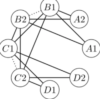
Forn= 8, considerP4. Draw edges between all theA’s andB’s etc. to get supergraphs. Now join the B and C vertices.

A1 A2 B1 B2 C1 C2 D1 D2

Figure 19: A construction for n= 8

Example. Is there a nontrivial disconnected self-complementary graph? Of course not.

7 February 13, 2013

7.2 Today’s topics Chapter 3:

Reconstruction Conjecture 7.3 Card Game

“I am thinking of a graph.”

Given the graph G, we are shown the induced subgraphsG− {v}for each v∈G. For our example:

Figure 20:Ghas order 6, and dropping each of the vertices yields the following figures. For this particular graph, it is not hard to use the fourth card to reconstruct the graph:

6 5

3 2

4 1

Figure 21: The solution to the problem

Definition. For any vertex v∈V(G), the graphG−v is called acard of G. Thedeck

of Grefers to the collection of all cards. 7.4 Reconstruction Conjecture

Is it possible to reconstruct the graphGfrom its deck?

In fact, there is a counter-example already at n= 2; note thatK2 andE2 have the same deck! So we modify this to give:

Problem (Reconstruction Conjecture). IfGhas at least three vertices, then Gcan be reconstructed from its deck.

7.5 Recognizable Properties

Definition. A property/parameter is called recognizable if it can be determined from the deck of a graph.

What properties are recognizable? Let there be ncards (i.e. Ghas ordern) and let the cards beC1, C2,· · · , Cn. Letmi be the size ofCi, and let m be the size ofG. Fact 7.1. The order is recognizable.

Proof. This is trivial.

Fact 7.2. The size is recognizable, and therefore the degree sequence. In particular, regularity is recognizable.

Proof. Observe that mi =m−degvi. Summing up, we find that X mi= X m−Xdegvi =nm−2m =⇒ m= 1 n−2 X mi.

Therefore we obtain m, and we can find the degree sequence by looking at each mi individually.

Fact 7.3. Connectedness is recognizable.

Proof. Apply Theorem 2.2 directly.

Fact 7.4. Being bipartite is recognizable;G is bipartite if and only if (i) All cards are bipartite, and

(ii) Gis not an odd cycle.

Proof. If Gis a cycle, then it’s trivial. If not, odd cycles are detected when any vertex not in the cycle is deleted.

Exercise. Show explicitly that the number of connected components ofGis recognizable by giving an algorithm.

7.6 Another Deck

Figure 22: Another deck. The solution is pretty clearly C5+K1.

7.7 Determining number of components in a deck Let’s take an example G=K4∪C3. We get

ˆ Four cardsC3∪C3.

ˆ Three cardsK4∪C2.

For a disconnected graph G, look at the largest connected component that appears among all the cards. Then we see that this must be a component of the original graph, and now we can go downwards!

8 February 18, 2013

ˆ Tress

Definition. n(G) will denote the order ofG, and m(G) will denote the size. Also,k(G) will denote the number of components.

8.2 Bridges

Definition. An edgeeis abridge if thek(G−e)> k(G). Example. In figure 23, the dotted edge is a bridge.

Figure 23: An example of a bridge. In Pn, every edge is a bridge. InCn, none of them are.

In this sense, none of the bridges in the Bay Area is actually a bridge.

Fact (Chartrand and Zhang, 4.1). Given a connected graph G, an edgee∈E(G) is a bridge if and only if e /∈C for any cycleC⊆G.

Proof. Clear. 8.3 Trees

Definition. A tree is an acyclic graph (i.e. without cycles).

Fact (Chartrand and Zhang, 4.2). A graph has a unique path between any two vertices if and only if it is a tree.

Proof. Clear.

Fact (Chartrand and Zhang, 4.3). T has at least 2 vertices of degree 1.

Proof. Consider a path of length diam(T). The endpoints must have degree 1. 8.4 The Size of a Tree and Consequences

Fact. In any tree,m(T) =n(T)−1.

Proof. Induction on n≥2. The base case n= 2 is clear. The inductive step n≥3 is obvious.

Definition. A forest is an acyclic graph. Note that it need not be connected; hence its components are trees.

Fact (Chartrand and Zhang, 4.6). For any forest F,m(F) =n(F)−k(F).

Proof. If F =T1∪T2∪ · · ·Tk for treesTi then X

1≤i≤k

m(Ti) = X 1≤i≤k

(n(Ti)−1).

Fact. IfGis a connected graph, then m(G)≥n(G)−1. Equality occurs if and only if

Gis a tree.

Proof. Cut open all the cycles inG to obtain a treeG0, where m(G0)≤m(G). But then

m(G0) =n(G)−1. Equality occurs only if no cycles were cut. Combining all of these results:

Theorem 8.1 (Characterization of Trees). Let G be a graph of order n and size m. Then any two of the following conditions imply the third:

(i) G is connected (ii) G is acyclic (iii) m=n−1

Furthermore, these conditions together imply G is a tree.

8.5 Spanning Tree

Definition. A spanning tree of a connected graph is a subgraph T ⊆ G for which

V(T) =V(G) and T is a tree.

Figure 24: A spanning tree, highlighted in red Now, Kn hasmany different spanning trees.

Fact 8.2. The number of labeled spanning trees of Kn isnn−2.

We can define the following matrices: The adjacency matrix is given by

A(G) :aij = ( 1 ifi,j adjacent 0 otherwise . D(G) :dij = ( degi if i=j 0 otherwise. Then define the Laplacian matrix L(G) =D(G)−A(G).

Theorem 8.3. Delete any row and column of L(G) to get a matrix L0(G). The number of spanning trees of G isdetL0(G), regardless of which row and column is selected.

9 February 20, 2013

ˆ Spanning trees

ˆ Minimal-weight spanning trees – Kruskel’s Algorithm – Prim’s Algorithm 9.2 Test 1 Synopsis

Test 1 on Monday. Six questions, 90 minutes. 1. Basic

2. Degree sequences (Hakimi-Havel) 3. Isomorphic Graph

4. Reconstruction Conjecture 5. Minimal-weight spanning trees

6. Proof: reproduce a proof either presented in class or on the homework 9.3 Spanning Trees

We have already seen that a graph contains “many” spanning trees.

Theorem 9.1 (Chartrand and Zhang, 4.10). Every connected graph has a spanning tree. Proof 1. Cut open any cycles. The result is a spanning tree.

Proof 2. Start with a trivial graph v. Pick edges incident with v to form a connected subgraphH. Continue to pick edges joiningV(H) and V(G−H). Eventually we get a connected graph withn−1 edges, so this is a spanning tree.

Proof 3. Start with an edge in E(G). Beginning with the empty graph onV(G), keep adding edges in such a way as to avoid cycles, untiln−1 edges have been added.

The second and third proofs are the basic idea for Prim’s Algorithm and Kruskel’s Algorithm, respectively.

9.4 Weighted Graphs First, definitions.

Definition. A weighted graph is a graph with a weight functionw:E(G)→_R. Often the range is actually Z.

Definition. Given a subgraphH ofG, theweight of H is defined as P

9.5 Minimum Weight Spanning Tree Problem

Problem. Given a weighted connected graphGwith weight functionw, find the minimum possible weight of a spanning tree.

Note that this is well-defined, since the set of spanning trees is finite and nonempty. The two algorithms presented here are greedy.

3 6

1 3

7

2 2

Figure 25: An example of a graph. Spanning tree is the solid line. As another example, consider the following graph.

A B C D E 1 4 3 2 3 1 2 2 4 5

Figure 26: Another graph; spanning tree is colored red.

9.6 Kruskal’s Algorithm

Algorithm 9.2 (Kruskal). Given a weighted connected graph,

ˆ Start with an edge with minimum weight.

ˆ Add edge with minimum weight from the remaining edge while avoiding cycles.

ˆ Repeatn−2 times.

For the graph given in figure 26, the following sequence produces a spanning tree. A possible example follows:

1. Pick edge AB. 2. Pick edge BD. 3. Pick edge BE. 4. Pick edge DC.

Before giving the proof, let us make some observations. Let {e1, e2,· · · , en−1} be the edges, in order.

We observe thatG({e1, e2,· · · , ei}) is a forest for all i. Also, we need the following lemma.

Lemma 9.3. Let T be a spanning tree of a connected graph G. IF e /∈ E(T), then

∃f ∈E(T) such that

T0=T−f+e is a spanning tree.

We actually need the idea in the proof, not the lemma itself.

f e

Figure 27: An example of the lemma. Spanning tree in red.

Proof of 9.2. Suppose Tk is generated by Kruskal’s, with edges Ek= (e1, e2,· · · , en−1) in that order, but is not a minimum weight spanning tree.

Then∃T withw(T)< w(Tk) such thatE(T) containse1,· · · , ei but notei+1; pick the

T where thisiis maximal. We will now construct a spanning treeT0withw(T0)< w(TK), and moreover, E(T0) containse1, e2,· · · , ei, e+i+ 1; this will give a contradiction.

We “invoke” the lemma. Sinceei+1 ∈/T, we can find an f ∈T such that

T0 =T −f+ei+1

is a spanning tree, andf /∈ {e1,· · · , ei}. This is possible because in the lemma we pickf from a cycle, and there is no cycle containing all edges in Ek.

WE claim that w(T0)< w(Tk). It suffices to prove that w(f)≥w(ei+1). If this is not the case, we havew(f)< w(ei+1); but this is impossible because we picked the edges greedily! (There is no cycle sincee1,· · · , ei, f ∈T.)

9.7 Prim’s Algorithm

Algorithm 9.4 (Prim’s Algorithm). Given a connected graph G,

ˆ Start with a trivial graph H on an arbitrary vertex.

ˆ Among all edges betweenV(H) and V(G−H), pick one with the minimal weight and add it to form a newH.

ˆ Repeat until V(H) =V(G).

The result is a minimal weight spanning tree.

10 Test 1 Solutions

Recorded here are the distinct solutions.

3. Considering diameters also works. Planarity works for 3b. Bipartite also works. Theorem 10.1. If G is a connected graph with all edges having all distinct weight then the minimal spanning tree is unique.

11 March 4, 2013

(finishes that fairly long homework exercise) 11.1 Today’s Topics Chapter 5: ˆ Cut vertex ˆ Nonseparable graph ˆ blocks 11.2 Cut vertices

Definition. v is a cut vertex of Gifk(G−v)> k(G). Example. Cn has no cut vertices (n≥3).

Example. K1,n has exactly one cut vertex (n≥2). Example. Pnhas n−2 cut vertices (where n≥3). Question. Is there a graph with all cut vertices? 11.3 Consequences

Fact 11.1 (Chartrand and Zhang, 5.1). Ifuv is a bridge of a connected G, thenv is a cut vertex if and only if degv≥2.

Proof. Clear.

Easy consequences:

ˆ Non end-vertices of a tree are cut vertices.

ˆ IfG has order at least 3, andGhas a bridge, then Ghas cut vertex.

Fact 11.2 (Chartrand and Zhang, 5.3). Letv be a cut-vertex of a connected graph G. Ifu, w lie in different components ofG−v thenv must be on every u−w path inG. Fact 11.3 (Chartrand and Zhang, 5.4). Ifv lies on everyu−w path in G, thenv is a cut-vertex.

Fact 11.4 (Chartrand and Zhang, 5.5). Let Gbe the connected graph. Letvbe a vertex such that

d(u, v) = max

x∈V(G)d(u, x) Then v is not a cut vertex.

Proof. Ifv is a cut vertex,∃w no longer connected tou. But then a geodesic u−wmust pass throughv, sod(u, w)> d(u, v)≥d(u, w) which is a contradiction.

Corollary 11.5 (Chartrand and Zhang, 5.6). Every nontrivial connected graph has at least 2 non-cut-vertices.

Corollary 11.6. If G is nonempty, then k(G) = min

v∈V(G)k(G−v).

Proof. Let C be a component of G, and C nonempty. Then ∃x ∈ V(C) such that

k(C−x) =k(C). In that casek(G−x) =k(G). But clearly,k(G−v)≥k(G) for anyv, so we’re done.

12 March 6, 2013

Definition. A nontrivial connected graph without cut-vertices is called nonseparable. Example. Cn andKn are nonseparable.

Fact 12.1 (Theorem 5.7). If|G| ≥4, thenGis nonseparable if and only if every pair of distinct vertices shares a common cycle.

Proof. In book.

Definition. A nontrivial connected graph with at least one cut-vertex is called separable. 12.3 Blocks

The intuition is that separable graphs will consist of “combinations” of nonsepara-ble graphs (“blocks”) in the same way that disconnected graphs consist of connected components. A B C D E F G H I J K L

Figure 28: A connected graph. The blocks are ABCD, CEF H, G, HIJ andJ KL. Cut vertices are highlighted.

Definition. Let G be connected. Define a relation ∼ onE(G): e∼f if and only ife

and f share a common cycle. For each equivalence classE of ∼over E(G), we get a blockB =G[E].

Fact 12.2. Let B1,· · ·, Bk be the blocks of a connected G. Then, (i) E(Bi)∩E(Bj) =∅,

(ii) |V(Bi)∩V(Bj)| ≤1, and

(iii) If {v}=V(Bi)∩V(Bj), thenv is a cut-vertex.

Remark. Ifv is a cut vertex, then ∃i6=j :v∈V(Bi)∩V(Bj). 12.4 Vertex connectivity

Definition. U ⊆V(G) is called a vertex-cut ifG−U is disconnected.

Definition. SupposeGis not the complete graph, thenκ(G), the vertex connectivity of

G, is defined by

κ(G) = min

Vertex cutU|U|.

A vertex cut U0 which achieves this minimum is called aminimum vertex-cut. Furthermore, κ(Kn) =n−1.

Note that a disconnected graph has κ(G) = 0 since∅ works. IfGis connected but has a cut-vertex, thenκ(G) = 1. Conversely, if κ(G) = 1, thenGis eitherK2 or is connected with at least one cut-vertex.

Definition. Gisk-connected ifκ(G)≥k; i.e. the deletion of strictly less thankvertices will not disconnected the graph.

Example. 0-connected graphs consists of all graphs. 1-connected graphs are connected graphs.

12.5 Edge-connectivity

Definition. X ⊆E(G) is called an edge-cut if G−X is disconnected. Definition. λ(G) is defined by

λ(G)def= min X edge-cut|X|

forG6=K1. We defineλ(K1) = 0. An edge-cut which achieves the minimum is called an

minimum edge-cut.

Example. λ(G) = 0 if G is disconnected, and λ(G) = 1 if G is connected and has a bridge. Also,λ(Kn) =n−1 (just delete all the edges of a vertex). This is not entirely trivial.

Claim. IfKn−X is disconnected, thenX ≥n−1.

Proof. Consider the complement. If Kn−X is disconnected, then Kn−X must be connected, so

|X|=m Kn−X

≥n−1 as desired.

In fact, more is true:

Theorem 12.3 (Chartrand and Zhang, 5.11). For any graphG, κ(G)≤λ(G)≤ min

Proof. First, we will show that λ(G) ≤δ(G), where δ is the minimum degree function. Assume thatv∈V(G) is such that degv =δ(G). Then just cut all the edges of v.

Next, to show κ(G)≤λ(G), consider a minimum edge-cut X0. Let us assume thatG is connected and is notKn (otherwise check the conclusion); evidentlyn≥3. Remark thatG−X0 has exactly 2 components; otherwise, we could find a smaller edge-cut X00, contradiction. LetG−X0=G1∪G2.

Now, we claim that ∃u ∈V(G1), v ∈V(G2) such that uv is not an edge. Note that

G6=Kn, soδ(G)≤n−2. If this is false, then

|X0|=|V(G1)| |V(G2)| =k(n−k)

Observe 1≤k≤n−1 since G1 andG2 are nontrivial. Yet |X0| ≤δ(G)≤n−2. It is easy to check that this is impossible.

Now take

13 March 11, 2013

14 March 13, 2013

Sufficient condition for Hamiltonian cycles. 14.2 Necessary Conditions

Definition. A graph isHamiltonian if it contains a Hamiltonian cycle; i.e. a cycle using every vertex once.

The graphG must satisfy 1. Connected

2. δ(G)≥2 3. n≥3

4. k(G−S)≤ |S|for all S⊆V(G). In particular, there are no cut vertices. 14.3 Sufficient conditions

Unfortunately, there are no necessary and sufficient conditions. Here are some sufficient conditions.

Fact(Chartrand and Zhang, 6.6). LetGbe a graph of order at least 3. If degu+degv≥n

for any nonadjacent u, v∈V(G) thenG is Hamiltonian.

Proof. Fix n. Consider a counterexampleH with ordern and maximal size; that is,H

is non-Hamiltonian. Clearly H6=Kn.

Then∃u, v such that H+uv becomes Hamiltonian. This implies there exists a path Hamiltonian path from u to v, as If ∃i such that uwi+1, uiw ∈ E(H) then this is a

u=w1 w2 w3 · · · wi wi+1 · · · v=wn

Figure 29: Hamiltonian Paths

contradiction, because then we can get a Hamiltonian cycle. But degu+ degv≥nso can be shown using Pigeonhole!

Actually, we can modify this to read

Fact (Chartrand and Zhang, 6.8). If u, v non-adjacent satisfy degu+ degv ≥ n, the nH+uv is Hamiltonian if and only if H is Hamiltonian.

14.4 Partial Closures

The above theorem motivates the following definition.

Definition. The partial closureG0 ofGis obtained fromGby adding all edgesuv where degu+ degv≥n.

Example. The partial closure of C5 is itself. The closure ofK5,5 isK10. An additional example is given below.

Figure 30: A graphG. Red edges comprise the first partial closure.

Definition. The complete closure ofC(G) ofG is obtained by taking partial closures until the graph stops changing; i.e.

C(G) = lim r→∞G 00_{· · ·}0 | {z } rtimes .

Example. Consider a graphG with degree sequence 9,6,6,6,5,5,5,5,4. Is it Hamilto-nian?

So clearly we want to use closures. Anyways here is something that kills it. 14.5 A sufficient criterion with degree sequences only

Theorem 14.1. Let |G| ≥3. If for every integer j < n₂, there are strictly less than j vertices with degree at most j, then H is Hamiltonian. In fact C(G) =Kn.

Proof. Suppose C(G)6=Kn. Then ∃u, w∈C(G) such that degu+ degw≤n−1. Take the pair such that degu+ degw ismaximal. Without loss of generality degu≤degw. Setk= degu; thenk= degu < n₂, and degw≤n−1−k.

Claim. Ifv and ware not adjacent, then degv ≤k.

Proof of Claim. Considervsuch that v andware not adjacent. Clearly degv+ degw≤

n−1 since this a closure. We claim that degv ≤ k. Otherwise, degv > k and degv+ degw >degu+ degw, contradicting maximality.

So every non-neighbor of whas degree at mostk. But there are at leastn−degw > k

of them. Since degrees increase under closure, and we havek≤ n−₂1, this contradicts the assumption.

15 March 18, 2013

ˆ Digraph

ˆ Oriented graph 15.2 Digraphs

A digraph is a directed graph.

Definition. D= (V, E) is digraph (directed graph) where V is the vertex set andE is the arc set.

As usual, loops are still not permitted.

Definition. The out degree of a vertex v, denoted od(v), is the number of verticesx for which vx∈E. The indegree of a vertex, denoted id(v) is the number of verticesx for which xv ∈E.

As usual, we have the provisos 0≤od(v)≤n−1 and 0≤id(v) ≤n−1. Now note that in a diagraph it is possible for all the indegrees to be distinct.

Fact (First Theorem for Digraphs). Let D be a digraph with n vertices and m arcs. Then X v∈V(D) id(v) = X v∈V(D) od(v) =m. Proof. Clear.

Finally, remark that a nontrivial (directed) cycle with two edges exists. 15.3 Digraph analogs of concepts in graphs

v1 v2 v3 v4

w v

Figure 31: An example of a digraph As usual, we have a directed walk/trail/path/circuit/cycle.

Fact. Any directed walk can be contracted to a directed path. In particular, any directed circuit can be contracted to a directed cycle

Definition. A digraph isconnected if the underlying graph is connected.

Definition. A digraph is strong (or strongly connected) if there exists a u−v directed path for anyu6=v.

Fact. Dis strong if and only if Dhas a spanning directed closed walk.

Proof. If there is a spanning directed closed walk, then D is clearly strong. For the converse just take directed pathsv1−v2− · · · −vn−v1. (Note that a cycle is different from a walk!)

15.4 Eulerian Circuits

Definition. A digraph D is Eulerian if there is a directed circuit which contains all edges ofD.

Fact. Dis Eulerian if and only if od(v) = id(v) for all v∈V(D).

Proof. Trivial.

15.5 Orientable Graphs

Definition. An orientable graph is a directed graph with no parallel arcs. This can be seen as an undirected graph with an orientation imposed on it.

Question. For whatGis it possible to orient a graph Gsuch that the resulting digraph is strong?

For example, the following graph, no orientation exists that works:

Figure 32: A graph whose orientations are all not strong. In fact, we have the following theorem.

Theorem. Given a nontrivial connected G, then there exists a strong orientation forG, if and only if G has no bridges.

Proof. If we have a bridge in G, then clearly we are doomed.

The converse is to basically keep adding cycles. Suppose every edge is part of a cycle. Take

S def= {S ⊆V(G) :G[S] has a strong orientation} where G[S] denotes the subgraph induced byS.

Note thatS 6=∅ because there exists a cycle in G. Not let

pdef= max{|S|:S ∈ S} ≥n.

Suppose that p6=nand consider a set S with|S|=p.

ConsiderS andG−S. There are at least two edges joining them since there are no bridges. Now direct S, and then add direction for any cycle starting/ending inS and having all other vertices inG−S. Then we get a bigger S, contradiction.

16 March 20, 2013

ˆ Tournament 16.2 Definitions

Definition. A tournament is a complete graph with an orientation.

Figure 33: The tournaments on 3 vertices.

There are two tournaments on two vertices and four on four vertices, up to isomorphism. 16.3 Transitive tournaments

Definition. A tournament T is called transitive ifux, xv∈E(T) =⇒ uv∈E(T). This definition is very rigid, as follows.

Fact. A tournamentT is transitive if and only ifT has no directed cycles. The proof is a triviality.

Fact. A tournamentT is transitive if and only if the out-degree sequence (or in-degree sequence!) is{0,1,2,· · · , n−1}.

Remark. There is only one transitive tournament of a given ordern, up to isomorphism. So transitive tournaments are not terribly interesting, because it’s just a strict ordering on the vertices. Here is something less trivial.

16.4 Spanning paths and cycles

Fact (Chartrand and Zhang, 7.8). Every tournament has a spanning directed path (i.e. Hamiltonian path).

Before giving the proof, we give a definition.

Definition. Given a directed path in a digraph, the length is 1 less than the number of vertices (analogous to the graph definition.)

Proof. Take the longest directed path P =v1 →v2 → · · · → vk and consider a vertex

v not inP (if it exists; otherwise we win). Clearly v→vk otherwise P0 =v1 → · · · →

vk→v is longer. Then, v→vk−1 since otherwisev1→ · · · →vk−1 →v→vk is longer. Proceeding analogously, we find thatv →vi for all i.

In particular, v→v1. But then v→v1→ · · · →vk is longer again, contradiction. Fact (Chartrand and Zhang, 7.10). A tournament T has a spanning directed cycle if and only if T is strong.

Proof. If T has a cycle we are done. Conversely, if T is strong, thenT is not transitive so there is a cycle. Take the longest cycleC now. If |C|< nthen there exists v not inC.

Suppose C=v1 →v2 → · · · →vk →v1. If ∃v→vi, vi+1 →v, where v /∈C, then we die because we get a longer cycle. So, for every x /∈V(C), either V(C) ⊆Nout(V) or

V(C)⊆Nin(V).

Let X be the set of vertices which all dominate V(C) and Y be the set of vertices which all are dominated by V(C). In other words

X→V(C)→Y

Since it’s strong, X and Y must be non-empty. Furthermore, there must be an edge

y→x where x, y∈X, Y; this is because T is strong again. But now x→v1→v2· · · →

vk→y→x is a cycle.

This is a longer cycle, so contradiction! 16.5 A parting shot

Question. Do there exist two tournaments not isomorphic with the same degree se-quence?

17 April 8, 2013

ˆ Matching

ˆ Matching in bipartite graphs

ˆ Hall’s Theorem 17.2 Matchings

Here is a motivating example! Consider six studentsA, B, C,D, E,F, with seven books

a, c, d, g, h, p, t. A B C D E F a c d g h p t

Figure 34: A bipartite graph and a matching on it.

Is it possible for all six students to pick a book without repetition? For this graph the answer is yes; the construction is red.

Definition. Given a graph G,M ⊂E(G) is called a matching of Gif the edges in M

share no common end-points.

Definition. A matchingM is perfect ifV(M) =V(G) Remark. This is of course only possible ifGhas even order.

Question. How can you tell whether a graph has a perfect matching? 17.3 Hall’s Marriage Theorem

Definition. A bipartite graph with left-hand and right-hand sets U and W will be denoted as B(U, W).

Definition(Hall’s Condition). A bipartite graphG=B(U, W) satisfiesHall’s Condition

if

|N(X)| ≥ |X| for allX ⊆U

Note that this is not symmetric with respect toU and W.

Theorem 17.1(Hall’s Marriage Lemma). A bipartite graphG= B(U, W)has a matching of cardinality|U|if and only if it satisfies Hall’s condition. In particular, when|U|=|V|

this matching is perfect.

Proof. It is obvious that Hall’s condition is necessary. We will prove the other direction using induction on|U|. The base case is trivial.

Assume that any bipartite graph G1 = B(U1, W1) with |U1| < k satisfying Hall’s condition has a perfect matching. Consider a bipartite graphG=B(U, W) such that |U|=kand Gsatisfies Hall’s condition.

Let us say that Gsatisfies thestrong Hall condition if|N(X)| ≥ |X|for any |X| ≥1 andX ⊂U (in particular X6=U). We may assume Gdoes not satisfy this property, for otherwise we may simply delete an arbitrary edgeeof G, and apply Hall’s theorem to

G−e.

Otherwise let us assume that there exists a nonempty proper subset X0 ⊂U with |X0|=|N(X0)|. Define

F =B(X0, N(X0))

H=B(U −X0, W−N(X0))

Now,F satisfies Hall’s condition because Gdoes as well. But now we claim H satisfies Hall’s condition. ConsiderS ⊆U −X0. Then, we obtain

NH(S) =NG(S)−NG(X0) =NG(S∪X0)−NG(X0) which implies

|NH(S)|=|NG(S∪X0)| − |NG(X0)| ≥ |S|+|X0| − |NG(X0)|=|S|.

So Hall’s condition applies, and we may match bothF and H. But the right-hand sets of F and H are disjoint. Hence Gcontains a perfect matching.

18 April 10, 2013

ˆ Consequences of Hall’s Theorem

ˆ Tutte’s Condition

ˆ Existence of 1-factor 18.2 Assorted Corollaries

Corollary (Chartrand and Zhang, 8.4). Let S={S1, S2,· · ·, Sn} be a family of finite

sets. Then S has a system of distinct representatives which are pairwise distinct if and only if the union of anyk sets Si has at least k elements.

Proof. Direct consequence of Hall’s Theorem.

Corollary (Marriage Theorem). Consider r ladies and r gentlemen. Then every subset of k ladies is collectively acquainted with at leastk gentlemen if and only if every subset of k gentlemen is also collectively acquainted with at least k ladies.

Proof. Both are equivalent to there existing a perfect matching by Hall’s Theorem. Corollary. Everyr-regular bipartite graph has a perfect matching.

Proof. LetG=B(U, W). Then the size ofG is equal to bothr|U|andr|W|, implying |U|=|W|.

Then for each X ⊆U, there arer|U|edges, and each vertex inV incident to such an edge can accept at mostr edges. Hence

|N(X)| ≥ r|X|

r =|X|

and we are done by Hall’s Theorem. 18.3 Factors

Definition. A factor of a graph Gis a spanning subgraph of G. It is called anr-factor

if it is also r-regular.

For example, any Hamiltonian path/cycle is a factor.

Furthermore, a 1-factor corresponds directly to a perfect matching. Example. The Peterson graph, K2×C5 and H3,10 each contain 1-factors.

Secondly, a 2-factor corresponds to a spanning collection of disjoint cycles. Example. The Peterson graph, K2×C5, andH3,10 also have 2-factors.

18.4 Tutte’s Condition

How do we determine whether a graph has a 1-factor? In fact, there is a characterization, as follows. First let us defineTutte’s condition as follows.

Definition. Let ko(H) denote the number of odd components of a graphH.

Definition (Tutte’s Condition). A graph satisfiesTutte’s condition ifko(G−X)≤ |X| for everyX ⊆V(G).

Theorem (Chartrand and Zhang, 8.10). A graphG has a 1-factor if and only if Tutte’s condition is satisfied.

Proof. Deferred to MATH 279. As a consequence, we have

Fact. Every connected 3-regular graph without bridges contains a 1-factor.

Proof. We use Tutte’s Theorem. Suppose thatG−Xhas odd componentsG1, G2,· · · , Gk. For eachGi, let Ei be the set of edges joining a vertex ofX to a vertex of Gi. Then

3|Gi|=|Ei|+ 2m(Gi).

SinceGi is an odd component, we see that|Ei|is odd. Since there are no bridges, it is not the case that|Ei|= 1. Therefore,|Ei| ≥3.

Hence, there are at least 3kedges joining a vertex ofXto someEi. SinceX is 3-regular inG, it follows that|X| ≥ 3k

3 =k. Then by applying Tutte’s Theorem we are done. 18.5 More on factors

Definition. A graph G is 1-factorable if E(G) is the disjoint union of edges from 1-factors.

Example. Figure 35 shows a 1-factoring ofK4 by colors.

Figure 35: A 1-factoring ofK4. The three matchings each have their own color.

Fact (Chartrand and Zhang, 8.13). The Peterson graph is not 1-factorable.

Proof. Suppose on the contrary that this is the case; that is

E(P G) =M1∪M2∪M3.

ThenHdef= M2∪M3 is a 2-factor; that is, a union of disjoint cycles. ButP Ghas girth 5 and does not have a Hamiltonian cycle, so we must have H=C5∪C5. But thenM2 is a subgraph ofH which is not possible.

19 April 15, 2013

ˆ F-factorable graph

ˆ Kirkman’s Schoolgirl Problem 19.2 F-factorable graph

As stated last time,

Definition. G is 1-factorable ifGis a disjoint union of 1-factors. Example. K4 is 1-factorable, but the Peterson graph is not.

We generalize this to arbitrary subgraphs.

Definition. Let F be a subgraph ofG. Then Gis F-factorable if

E(G) =E(F1)∪E(F2)∪ · · · ∪E(Fk)

where the union is disjoint, and each Fi is a subgraph of Gisomorphic to F. Example. K4 isP4-factorable.

Figure 36:K4 isP4-factorable andK5 isC5-factorable. Obviously,m(F)|m(G) is necessary but not sufficient.

19.3 Kirkman Schoolgirl Problem

Fifteen young ladies in a school walk out three abreast for seven days in succession: it is required to arrange them daily so that no two shall walk twice abreast.

Let us consider the case instead of nine girls.

Problem(Kirkman with nine girls). A school mistress has 9 schoolgirls whom she wishes to take on a daily walk. The girls are to walk in 3 rows of three each. It is required that no two girls should walk in the same row twice. How many days can it be done?

This is fairly doable for nine girls.

1 2 3 4 5 6 7 8 9

1 2 3 4 5 6 7 8 9

Figure 37:K9 and some of its 3K3 factors.

We can construct by taking the sets {1,2,3}, {1,4,7},{1,5,9}, {1,6,8} for the partners of 1, and then operate cyclically; these correspond to “diagonals”, “rows” and “columns”.

Now for the graph theory – each day corresponds to a 3K3-factor of K9. In other words, the problem is equivalent to showing that (3K3)-factorable.

To resolve Kirkman’s problem,

Theorem 19.1(Ray-Chaudhuri, Wilson). Kn is tK3-factorable if and only ifn= 6k+ 3

andt= 2k+ 1.

Proof. Necessity is trivial. Clearly we must have

m(tK3)|m(Kn) =⇒ 3t|

n(n−1) 2

by focusing on the number of edges. Also,Kn must have 3tvertices, hencen= 3t. Then 2|n−1 forces nodd and the conclusion is immediate.

19.4 Test 2

There will be six questions to be answered in 90 minutes. 1. Give example

2. Chapter 5: vertex/edge connectivity

3. Chapter 6: Eulerian and Hamiltonian circuits 4. Chapter 7: Digraphs, tournaments

5. Chapter 8: Matching in a bipartite graph 6. Proof

20 Test 2 Aftermath

ˆ Do not screw up the first question.

ˆ For 1d,H3,10 is a much cleaner solution.

21 April 24, 2013

Definition. A plane graph is a graph drawn in the plane without edge crossing. Definition. A planar graph is graph which can be drawn as a plane graph.

Example. K3 is a plane graph; K4 is a planar graph. However,K5 isnot planar. Also,

K2,3 is planar, but K3,3 is not.

Figure 38:K2,3 drawn planar

Surprisingly, K3,3 andK5 are the in fact the “root of all evil”! We can use them to characterize planar graphs.

Remark. Subgraphs of planar graphs are planar. 21.3 Euler and its consequences

Let us introduce the classic theorem of Euler.

Theorem 21.1(Euler). IfGis a connected plane graph of ordern, size m, andr regions, then

n−m+r = 2.

In fact, 2 is called the Euler characteristic ofS2.

Proof. By induction onm for fixed n. SinceGis connected, n−1≤m≤ n₂ .

If m = n−1, then G is a tree so there are no cycles and r = 1; this verifies the base case. Otherwise, there exists a cycle, so we just delete an edge from that cycle, reducing both m andr by 1 and hence preserving the quantity n−m+r, while leaving

Gconnected.

We can use this to restrict m in a planar graph. Here is one such restriction. Let us first define the girth of a graph:

Definition. Thegirth of a graphGis the length of a smallest cycle if it exists; otherwise, it is +∞.

Theorem 21.2. If Gis a plane graph of order n, size m and girth g, then m≤ g(n−2)

g−2 .

Proof. It suffices to consider the case whereGis connected; otherwise we can simply add bridges to unite components until it is connected. In this wayg is unchanged because no now cycles are introduced.

For each of the r regions, there is a cycle of length at least g; since each edge is a member of exactly two regions we obtain the inequality

m≥# edges in some cycle≥ 1 2rg=

1

2(2 +m−n)g. Solving for m with the knowledgeg= 3 yields thatm≤ g(n_g−−₂2) as desired. Corollary 21.3. If G is a plane graph with n≥3 and size m thenm≤3n−6. Proof. IfGis a forest, thenm≤n−1≤3n−6. Otherwise, note thatg≥3 =⇒ _g−g₂ ≤ 3.

Remark. As a result ofm≤3n−6, planar graphs are asymptotically sparse sincem is bounded byO(n).

Using these results, it is easy to check that K5 andK3,3 are nonplanar.

Remark. In amaximal planar graph of order n, all regions must be triangles. In fact these are constructible; here is a maximal graph withn= 5.

Figure 39: A maximal n−5 graph

21.4 Subdivisions

The Peterson Graph is nonplanar. Who’s responsible?

Definition. A graphG0 is called asubdivision ofG0can be obtained fromGby replacing some edges with path graphs.

This definition is useful because a graph and its subdivision are either both planar and both nonplanar.

Here is a deep result.

Theorem 21.4 (Kuratoski). A graph Gis planar if and only if it contains a subdivision of K5 and K3,3.

7→

Figure 40: Trading

Figure 41: The left graph is a subdivision of the right graph

21.5 Another Question

Question. Is it possible that both Gand Gare nonplanar?

Clearly this cannot hold for large enough n, since maxm(G), m(G) =O(n2). Work-ing out the details, we have

n

2

=m(G) +m(G)≤6n−12 =⇒ n2−13n+ 24≤0 =⇒ n≤10.

So whichn are actually constructible?

The cases n≤4 are easy. For n= 5, we can take G=C5. For n= 6, we may take

G=K2∪K4.

It turns out that n∈ {7,8} are possible, butn∈ {9,10} are not. The casesn∈ {7,8} can be achieved by takingG as a maximal planar graph.

22 April 29, 2013

22.2 Contraction and Minors

Definition. Consider an edge e=uv∈E(G) in a graph G. Then the graph obtained from the contraction ofeis G0 def= G−v, with the additional edges{ux:x∪N(v)}.

a b c d

Figure 42: The edge cdis contracted.

Example. Kn with any edge contracted results inKn−1.

Definition. H is a minor of G if H can be obtained from G by a finite sequence of deletion of vertices/edges and/or contraction of edges, in any order.

Example. Here are some obvious examples. 1. K1 is a minor of any nontrivial graph. 2. Any subgraph of a graph is a minor. 3. K5 is a minor ofKt ifs≤t.

Example. K5 is a minor of the Peterson Graph.

Example. K3,3is a subdivision of PG. This follows from the fact that PG is a subdivision of K3,3. 2a 5 3a 2b 1b 4 3c 3b 6 1a 4 5 1 2 3 6

c b a d e x y

Figure 44:K5 is a minor ofC5+K2. Contract the red edges. The edges betweenC5 and

K2 are dashed for clarity.

22.3 Properties of Minors

Fact. IfGis planar, then any minor of Gis also planar. Fact. IfGis a subdivision of H, thenH is a minor ofG.

Note that the converse of this is not true. The operations one can make going from a graphG to its minor is a strict subset of form a subdivision of a graphG toG.

Minors are useful because of the following theorem.

Theorem 22.1 (Wagner). G is non-planar if and only ifK5 or K3,3 is a minor of G.

Proof. Long, although shortened by invoking Kuratoski. 22.4 Forbidden Graphs

Definition. A property P is said to be minor-hereditary ifG has propertyP, then any minor of Galso has property P.

Example. Planarity is minor-hereditary. Being a forest is also minor-hereditary. Definition. A graph is said to be outer-planar if the graph can be drawn as a plane graph such that every vertex touches the outer region.

Note thatK4 is not outer-planar.

Figure 45: An outer-planar graph

Theorem 22.2 (Robertson-Seymour). Given an infinite sequence of graphs, there are two graphs Gand H such that G is a minor of H. In other words, this is a quasi-well ordering.

Proof. Twenty papers spanning over 500 pages.

Corollary 22.3. If P is a minor-hereditary property, then there exists a finite family of graphs {H1, H2,· · · , Hk} for which the following statement holds:

G has property P if and only if none of the Hi are a minor of Gfor any i.

Proof. Consider the setS of graphswithout property P. Let

F ={G∈S:@H∈S a minor ofG}.

By Robertson-Seymour, F must be finite. Now, F is the forbidden set – since P is minor-hereditary, any graph with propertyP cannot contain any of the forbidden graphs inF.

Example. 1. Gis planar if and only ifK5 and K3,3 are not minors of G. 2. Gis a forest if and only ifC3 is not a minor of G.

3. Gis outer-planar if and only if K4 orK2,3 is not a minor ofG.

There is an analogous result for properties for vertex-induced subgraphs. In this case, the forbidden family may be infinite.

23 May 1, 2013

ˆ Definition of chromatic number

ˆ Examples

ˆ Lower bounds

ˆ Upper bounds 23.2 Motivation Here are some classes.

GT MA G AC LA S Student Signups Alice LA, S

Bob MA, LA, G Carol MA, G, LA

Figure 46: Graph theory, stats, linear alg, adv calculus, geometry, modern algebra

Question. Given a set of classes and the students taking each class, what is the smallest number of time slots needed?

This is basically a vertex coloring. 23.3 Vertex Coloring

Definition. Given a graph G, a k-coloring of G is an assignment of k colors to the vertices ofG such that no two adjacent vertices use the some color.

Definition. The chromatic number of Gis the minimum kfor which ak-coloring of G

exists. The chromatic number ofG is denoted byχ(G). Example. Some obvious chromatic numbers:

ˆ χ(Kn) =n

ˆ χ(Pn) = 2 (where n≥2)

ˆ χ(Cn) = 1₂(5 + (−1)n+1_{) (where n ≥ 3). In other words, χ(C2k) = 2, and}

χ(C2k+1) = 3.

Example. The Harary GraphH3,10 has chromatic number 2, because it is bipartite. Fact. A graphGis bipartite and non-empty if and only ifχ(G) = 2.

Proof. This is obvious.

Example. χ(C5×K2) = 3. Indeed, the chromatic number is at least 3 since it has on odd cycle in it, and a 3-coloring is not difficult to construct.

We can make this easy observation more explicit as follows. Fact. IfH is a subgraph of G, thenχ(H)≤χ(G).

So, in general, establishing a chromatic number can be done by find a constructing and getting the lower bound.

Fact. For any graphsG1 and G2, we have

χ(G1+G2) =χ(G1) +χ(G2).

Proof. This is obvious. Just check that G1 and G2 cannot share any colors.

Example. The graph in figure 46 is actuallyK1+C5. Soχ(K1+C5) =χ(K1)+χ(C5) = 4. 23.4 Lower Bound

Here are some easy lower bounds.

First, let us make the following definition.

Definition. The independence number of a graph G, denoted α(G), is the maximum number of vertices one can select fromGwith no edges among them. In other words, it is the size of the largest empty vertex-induced subgraph.

Example. The independent number for some canonical graphs are as follows:

ˆ α(Kn) = 1 for any n. ˆ α(Cn) = ₁ 2n for any n≥3. ˆ α(Pn) = ₁ 2n for any n≥2. Fact. χ(G)≥ n

α(G) for any graph G.

Proof. Interpret ak-coloring as a grouping ofG into independent setsS1, S2,· · · , Sk. It follows that n = Pk

i=1|Si| ≤ k·α(G), which implies the conclusion. In particular, if

k=χ(G) then we get the conclusion.

Definition. The clique number of a graph G, denoted ω(G), is the largestt for which

Kt is a subgraph ofG. Example. χ(Kn) =n. Also, ω(Cn) = ( 2 n≥4 3 n= 3. Additionally, ω(Pn) = 2 and ω(PG) = 2. Fact. χ(G)≥ω(G). Proof. χ(G)≥χ(K_ω(G)) =ω(G).

23.5 Upper Bound Fact. χ(G)≤n.

Proof. Please tell me you know how to prove this. Clearly the best way to get bounds is by construction. The greedy algorithm give us a bound as follows:

Fix a labelling ofV(G). Then color each vertex in order, adding a new color only if necessary.

Being the greedy algorithm, this may be suboptimal. For instance, consider a labelling of P4 as below:

1 4 3 2

Figure 47:P4, which has chromatic number 2, but the greedy algorithm produces a 3-coloring.

As a corollary of the algorithm, we may observe

χ(G)≤maxn )i=1

|N(vi)∩ {v1, v2,· · · , vi−1}|. In particular, since N(vi)≤∆(G) + 1, we have the weak bound Fact. χ(G)≤∆(G) + 1 for all graphs G.

However, this can actually be strengthened!

Theorem 23.1 (Brook’s Theorem). Let G be a connected graph. IfG is not Kn nor an

odd cycle, then λ(G)≤δ(G). Proof. 279A.

23.6 More examples

Exercise. Show that χ(PG) = 3.

Proof. χ(PG) ≤ 3 via Brook’s Theorem. On the other hand, χ(PG) ≥ 3 because it contains an odd cycle. Hence,χ(PG) = 3.

C B A F E D Y X

1 2 3 4

5 6 7 8

9 10 11 12 13 14 15 16 Table 2: 2×2 Sudoku

Exercise. Find the chromatic number of the graph shown in figure 48.

Proof. χ(G) = 4. Color chase with the bound χ(G)≥3 (because of the triangle). Exercise (Fake Sudoku). Consider the graphG on vertices {1,2,· · · ,16}, where two vertices are adjacent if they are in the same row, column, or 2×2 box (see figure 2). Find the chromatic number.

Proof. Clearly χ(G) ≥ 4 because there is a 4-clique. But a 4-coloring exists, because otherwise Sudoku would be a very boring game.

24 May 6, 2013

ˆ χ(G) versusχ(G)

ˆ Coloring maps 24.2 Examples

Question. How areχ(G) andχ(G) related?

Example. When G=C4, we have 2 and 2, respectively. When G=Kn, we have nand 1 respectively.

24.3 Relating chromatic numbers

Theorem 24.1. For any graph Gof order n, χ(G)χ(G)≥nand χ(G) +χ(G)≤n+ 1.

Notice that both bounds are tight in our example. It is not hard, however, to find instances where these bounds are not tight. For example, take the Peterson graph. Here

n= 10, χ(PG) = 5, and χ(PG) = 4

Proof. For the first part, note that

χ(G)χ(G)≥ n

α(G)ω(G) =

n

α(G)α(G) =n.

The second inequality is via induction on n. The base case isn= 1, which is trivial. For the inductive step, consider a graph G of order n+ 1. Take anyv ∈V(G); then

G−v is a graph of order n. By the induction assumption, we have

χ(G−v) +χ(G−v)≤n+ 1.

We want to compare χ(G−v) andχ(G). Obviously we have χ(G)≤χ(G−v) + 1, but this is not tight enough. However, if deg_Gv < χ(G−v), then this inequality must be strict – we simply pick a color that v is not adjacent to.

If either inequality is strict, then we can simply sum the inequalities to yield the desired. Otherwise, we must have deg_Gv≥χ(G−v) and deg_G(v) ≥χ(G−v). Then, taking both the inequalities as equalities gives

n+ 2> n+ 1 = 2 + (n−1) = 2 + deg_Gv+ deg_Gv ≥1 +χ(G−v) + 1 +χ(G−v) =χ(G) +χ(G) 24.4 Perfect Graphs

Definition. A graph G is called perfect if for every vertex-induced subgraph H of G, we have χ(H) =ω(H).

Theorem 24.2 (Perfect Graph Theorem, Lov´asz, 1972). G is perfect if and only if G is perfect.

Theorem 24.3 (Strong Perfect Graph Theorem). G is perfect if and only ifG does not contain C2k+1 or C2k+1 for anyk≥2.

24.5 Map coloring

Definition. A map is a region subdivided into smaller regions. Two subregions are

neighboring if they share a boundary line.

Remark. Utah and New Mexico are not neighbors because they intersect at only a single point.

Problem (The problem of 5 princes). Divide the kingdom into five pieces such that each prince’s region is adjacent to any other region.

Obviously this is not possible because of the four color theorem. For a flavorful description of this,

Problem (The problem of 5 palaces). Do the same, but draw a palace in each region and connect them with non-intersecting roads.

It’s easy to see the n-prince problem is equivalent to then-palace problem, son= 5 fails because K5 is not planar. Okay.

This idea results in the dual of a map.

Definition. Thedual of a map is the graph whose vertices are the faces are the regions of the map, and edges between any two neighboring/adjacent region.

It is easy to check that duals are planar. So the map coloring problem is simply the coloring of the planar graphs.

24.6 The 6-color problem and 5-color problem

Four colors is too hard. The six-color case, however, is immediate by the following lemma. Lemma 24.4. If G is planar, then δ(G)≤5.

Proof. E ≥3V −6, so P

v∈V degv <6V. This implies some vertex has degree less than 6, or at most 5.

Corollary. If Gis planar, then χ(G)≤6.

Proof. Induct on n ≥6. For the inductive step, take the vertex v of minimal degree. 6-color all other vertices and then apply a suitable color to v. Since degv ≤5 this is possible.

We can improve this.

Theorem 24.5. If Gis planar, then χ(G)≤5.

Proof. Induct on n≥5 this time. Take a vertex v with degree at most 5. If degv <5, then this is easy, since we can just 5-colorG−v as before.

On the other hand, suppose degv= 5. Since there cannot be aK5 among these 5, we may assume v1 andv3 are non-adjacent. Contracting edges vv1 and vv3, we obtain a graphH of ordern−2. Now 5-colorH. This implies there is a coloring scheme ofG−v