Optimal Multiserver Configuration for Profit
Maximization in Cloud Computing
Junwei Cao,
Senior Member, IEEE
Kai Hwang,
Fellow, IEEE
Keqin Li,
Senior Member, IEEE
Albert Y. Zomaya,
Fellow, IEEE
Abstract—As cloud computing becomes more and more popular, understanding the economics of cloud computing becomes critically important. To maximize the profit, a service provider should understand both service charges and business costs, and how they are determined by the characteristics of the applications and the configuration of a multiserver system. The problem of optimal multiserver configuration for profit maximization in a cloud computing environment is studied. Our pricing model takes such factors into considerations as the amount of a service, the workload of an application environment, the configuration of a multiserver system, the service level agreement, the satisfaction of a consumer, the quality of a service, the penalty of a low quality service, the cost of renting, the cost of energy consumption, and a service provider’s margin and profit. Our approach is to treat a multiserver system as an M/M/m queueing model, such that our optimization problem can be formulated and solved analytically. Two server speed and power consumption models are considered, namely, the idle-speed model and the constant-speed model. The probability density function of the waiting time of a newly arrived service request is derived. The expected service charge to a service request is calculated. The expected net business gain in one unit of time is obtained. Numerical calculations of the optimal server size and the optimal server speed are demonstrated.
Index Terms—Cloud computing, multiserver system, pricing model, profit, queueing model, response time, server configuration, service charge, service level agreement, waiting time.
F
1
I
NTRODUCTIONC
LOUD computing is quickly becoming an effec-tive and efficient way of computing resources and computing services consolidation [9]. By central-ized management of resources and services, cloud computing delivers hosted services over the Inter-net, such that accesses to shared hardware, software, databases, information, and all resources are provided to consumers on-demand. Cloud computing is able to provide the most cost-effective and energy-efficient way of computing resources management and com-puting services provision. Cloud comcom-puting turns in-formation technology into ordinary commodities and utilities by using the pay-per-use pricing model [3], [5], [16]. However, cloud computing will never be free [8], and understanding the economics of cloud • J. Cao is with the Research Institute of Information Technology, Tsinghua National Laboratory for Information Science and Technology, Tsinghua University, Beijing 100084, China.E-mail: [email protected]
• K. Hwang is with the Department of Electrical Engineering, Univer-sity of Southern California, Los Angeles, CA 90089, USA.
E-mail: [email protected]
• K. Li is with the Department of Computer Science, State University of New York, New Paltz, New York 12561, USA.
E-mail: [email protected] This is the author for correspondence.
• A. Y. Zomaya is with the School of Information Technologies, Univer-sity of Sydney, Sydney, NSW 2006, Australia.
E-mail: [email protected]
computing becomes critically important.
One attractive cloud computing environment is a three-tier structure [13], which consists of infrastruc-ture vendors, service providers, and consumers. The three parties are also called cluster nodes, cluster managers, and consumers in cluster computing sys-tems [19], and resource providers, service providers, and clients in grid computing systems [17]. An in-frastructure vendor maintains basic hardware and software facilities. A service provider rents resources from the infrastructure vendors, builds appropriate multiserver systems, and provides various services to users. A consumer submits a service request to a service provider, receives the desired result from the service provider with certain service level agreement, and pays for the service based on the amount of the service and the quality of the service. A service provider can build different multiserver systems for different applications domains, such that service re-quests of different nature are sent to different mul-tiserver systems. Each mulmul-tiserver system contains multiple servers, and such a multiserver system can be devoted to serve one type of service requests and applications. The configuration of a multiserver system is characterized by two basic features, i.e., the size of the multiserver system (the number of servers) and the speed of the multiserver system (execution speed of the servers).
Like all business, the pricing model of a service provider in cloud computing is based on two com-ponents, namely, the income and the cost. For a
service provider, the income (i.e., the revenue) is the service charge to users, and the cost is the renting cost plus the utility cost paid to infrastructure ven-dors. A pricing model in cloud computing includes many considerations, such as the amount of a service (the requirement of a service), the workload of an application environment, the configuration (the size and the speed) of a multiserver system, the service level agreement, the satisfaction of a consumer (the expected service time), the quality of a service (the task waiting time and the task response time), the penalty of a low quality service, the cost of renting, the cost of energy consumption, and a service provider’s margin and profit. The profit (i.e., the net business gain) is the income minus the cost. To maximize the profit, a service provider should understand both service charges and business costs, and in particular, how they are determined by the characteristics of the applications and the configuration of a multiserver system.
The service charge to a service request is deter-mined by two factors, i.e., the expected length of the service and the actual length of the service. The expected length of a service (i.e., the expected service time) is the execution time of an application on a standard server with a baseline or reference speed. Once the baseline speed is set, the expected length of a service is determined by a service request itself, i.e., the service requirement (amount of service) measured by the number of instructions to be executed. The longer (shorter, respectively) the expected length of a service is, the more (less, respectively) the service charge is. The actual length of a service (i.e., the actual service time) is the actual execution time of an application. The actual length of a service depends on the size of a multiserver system, the speed of the servers (which may be faster or slower than the baseline speed), and the workload of the multiserver system. Notice that the actual service time is a random variable, which is determined by the task waiting time once a multiserver system is established.
There are many different service performance met-rics in service level agreements [2]. Our performance metric in this paper is the task response time (or the turn around time), i.e., the time taken to complete a task, which includes task waiting time and task execu-tion time. The service level agreement is the promised time to complete a service, which is a constant times the expected length of a service. If the actual length of a service is (or, a service request is completed) within the service level agreement, the service will be fully charged. However, if the actual length of a service exceeds the service level agreement, the service charge will be reduced. The longer (shorter, respectively) the actual length of a service is, the more (less, respectively) the reduction of the service charge is. In other words, there is penalty for a service provider to break a service level agreement. If the
actual service time exceeds certain limit (which is service request dependent), a service will be entirely free with no charge. Notice that the service charge of a service request is a random variable, and we are interested in its expectation.
The cost of a service provider includes two com-ponents, i.e., the renting cost and the utility cost. The renting cost is proportional to the size of a multiserver system, i.e., the number of servers. The utility cost is essentially the cost of energy consumption and is determined by both the size and the speed of a multiserver system. The faster (slower, respectively) the speed is, the more (less, respectively) the utility cost is. To calculate the cost of energy consumption, we need to establish certain server speed and power consumption models.
To increase the revenue of business, a service provider can construct and configure a multiserver system with many servers of high speed. Since the actual service time (i.e., the task response time) con-tains task waiting time and task execution time, more servers reduce the waiting time and faster servers reduce both waiting time and execution time. Hence, a powerful multiserver system reduces the penalty of breaking a service level agreement and increases the revenue. However, more servers (i.e., a larger multiserver system) increase the cost of facility renting from the infrastructure vendors and the cost of base power consumption. Furthermore, faster servers in-crease the cost of energy consumption. Such inin-creased cost may counterweight the gain from penalty reduc-tion. Therefore, for an application environment with specific workload which includes the task arrival rate and the average task execution requirement, a service provider needs to decide an optimal multiserver con-figuration (i.e, the size and the speed of a multiserver system), such that the expected profit is maximized.
In this paper, we study the problem of optimal multiserver configuration for profit maximization in a cloud computing environment. Our approach is to treat a multiserver system as an M/M/m queue-ing model, such that our optimization problem can be formulated and solved analytically. We consider two server speed and power consumption models, namely, the idle-speed model and the constant-speed model. Our main contributions are as follows. We derive the probability density function of the waiting time of a newly arrived service request. This result is significant in its own right and is the base of our discussion. We calculate the expected service charge to a service request. Based on these results, we get the expected net business gain in one unit of time, and obtain the optimal server size and the optimal server speed numerically. To the best of our knowledge, there has been no similar investigation in the literature.
One related research is user-centric and market-based and utility-driven resource management and task scheduling, which have been considered for
cluster computing systems [7], [18], [19] and grid computing systems [4], [11], [17]. To compete and bid for shared computing resources through the use of economic mechanisms such as auctions, a user can specify the value (utility, yield) of a task, i.e., the reward (price, profit) of completing the task. A utility function, which measures the value and importance of a task as well as a user’s tolerance to delay and sensitivity to quality of service, supports market-based bidding, negotiation, and admission control. By taking an economic approach to providing service-oriented and utility computing, a service provider allocates resources and schedules tasks in such a way that the total profit earned is maximized. Instead of traditional system-centric performance optimization such as minimizing the average task response time, the main concern in such computational economy is user-centric performance optimization, i.e., maximiz-ing the total utility delivered to the users (i.e., the total user-perceived value).
The rest of the paper is organized as follows. In Section 2, we describe our queueing model for mul-tiserver systems. In Section 3, we present our server speed and power consumption models. In Section 4, we derive the probability density function of the wait-ing time of a newly arrived service request. In Section 5, we define a service charge function and calculate the expected service charge to a service request. In Section 6, we obtain the expected net business gain in one unit of time. In Section 7, we show how to obtain the optimal server size and the optimal server speed numerically. In Section 8, we demonstrate simulation data to validate our analytical results and to find more effective queueing disciplines. We conclude the paper in Section 9.
2
A M
ULTISERVERM
ODELThroughout the paper, we use P[e] to denote the probability of an evente. For a random variablex, we usefx(t)to represent the probability density function (pdf) of x, and Fx(t) to represent the cumulative distribution function (cdf) ofx, and¯xto represent the expectation of x.
A cloud computing service provider serves users’ service requests by using a multiserver system, which is constructed and maintained by an infrastructure vendor and rented by the service provider. The ar-chitecture detail of the multiserver system can be quite flexible. Examples are blade servers and blade centers where each server is a server blade [14], clusters of traditional servers where each server is an ordinary processor [7], [18], [19], and multicore server processors where each server is a single core [15]. We will simply call these blades/processors/cores as
servers. Users (i.e., customers of a service provider) submit service requests (i.e., applications and tasks) to a service provider, and the service provider serves
the requests (i.e., run the applications and perform the tasks) on a multiserver system.
Assume that a multiserver systemShasmidentical servers. In this paper, a multiserver system is treated as an M/M/m queueing system which is elaborated as follows. There is a Poisson stream of service re-quests with arrival rateλ, i.e., the inter-arrival times are independent and identically distributed (i.i.d.) exponential random variables with mean1/λ. A mul-tiserver system S maintains a queue with infinite capacity for waiting tasks when all the m servers are busy. The first-come-first-served (FCFS) queueing discipline is adopted. The task execution requirements (measured by the number of instructions to be exe-cuted) are i.i.d. exponential random variablesr with meanr¯. Themservers (i.e., blades/processors/cores) of S have identical execution speed s (measured by the number of instructions that can be executed in one unit of time). Hence, the task execution times on the servers of S are i.i.d. exponential random variables
x=r/swith meanx¯= ¯r/s.
Letµ= 1/x¯=s/r¯be the average service rate, i.e., the average number of service requests that can be finished by a server of S in one unit of time. The server utilization is ρ= λ mµ = λx¯ m = λ m· ¯ r s,
which is the average percentage of time that a server ofS is busy. Let pk denote the probability that there arekservice requests (waiting or being processed) in the M/M/m queueing system forS. Then, we have ([12], p. 102) pk= p0 (mρ)k k! , k≤m; p0 mmρk m! , k≥m; where p0= m−1 X k=0 (mρ)k k! + (mρ)m m! · 1 1−ρ !−1 .
The probability of queueing (i.e., the probability that a newly submitted service request must wait because all servers are busy) is
Pq = ∞ X k=m pk = pm 1−ρ =p0 (mρ)m m! · 1 1−ρ.
The average number of service requests (in waiting or in execution) inS is N = ∞ X k=0 kpk=mρ+ ρ 1−ρPq.
Applying Little’s result, we get the average task re-sponse time as T =N λ = ¯x 1 + Pq m(1−ρ) = ¯x 1 + pm m(1−ρ)2 .
The average waiting time of a service request is
W =T−x¯= pm
m(1−ρ)2x.¯
The waiting time is the source of customer dissatisfac-tion. A service provider should keep the waiting time to a low level by providing enough servers and/or increasing server speed, and be willing to pay back to a customer in case the waiting time exceeds certain limit.
3
POWER
CONSUMPTION
MODELS
Power dissipation and circuit delay in digital CMOS circuits can be accurately modeled by simple equa-tions, even for complex microprocessor circuits. CMOS circuits have dynamic, static, and short-circuit power dissipation; however, the dominant component in a well designed circuit is dynamic power consump-tionp(i.e., the switching component of power), which is approximately P =aCV2f, where a is an activity factor, C is the loading capacitance, V is the supply voltage, andf is the clock frequency [6]. In the ideal case, the supply voltage and the clock frequency are related in such a way thatV ∝fφ for some constant
φ >0[20]. The processor execution speedsis usually linearly proportional to the clock frequency, namely,
s ∝ f. For ease of discussion, we will assume that
V =bfφands=cf, wherebandcare some constants. Hence, we know that power consumption is P =
aCV2f = ab2Cf2φ+1 = (ab2C/c2φ+1)s2φ+1 = ξsα, where ξ=ab2C/c2φ+1 and α= 2φ+ 1. For instance, by setting b = 1.16, aC = 7.0, c = 1.0, φ = 0.5,
α= 2φ+ 1 = 2.0, andξ=ab2C/cα= 9.4192, the value of P calculated by the equationP =aCV2f =ξsα is reasonably close to that in [10] for the Intel Pentium M processor.
We will consider two types of server speed and power consumption models. In the idle-speed model, a server runs at zero speed when there is no task to perform. Since the power for speed s is ξsα, the average amount of energy consumed by a server in one unit of time is
ρξsα= λ
mrξs¯
α−1,
where we notice that the speed of a server is zero when it is idle. The average amount of energy con-sumed by anm-server systemS in one unit of time, i.e., the power supply to the multiserver systemS, is
P =mρξsα=λ¯rξsα−1,
wheremρ=λx¯is the average number of busy servers in S. Since a server still consumes some amount of power P∗ even when it is idle (assume that an idle server consumes certain base power P∗, which includes static power dissipation, short circuit power
dissipation, and other leakage and wasted power [1]), we will includeP∗ inP, i.e.,
P =m(ρξsα+P∗) =λrξs¯ α−1+mP∗.
Notice that whenP∗= 0, the aboveP is independent ofm.
In the constant-speed model, all servers run at the speed s even if there is no task to perform. Again, we use P to represent the power allocated to mul-tiserver system S. Since the power for speed s is
ξsα, the power allocated to multiserver system S is
P=m(ξsα+P∗).
4
WAITING
TIME
DISTRIBUTION
Let W denote the waiting time of a new service request that arrives to a multiserver system. In this section, we find the pdf fW(t) of W. To this end, we considerW in different situations, depending on the number of tasks in the queueing system when a new service request arrives. Let Wk denote the waiting time of a new task that arrives to an M/M/m queueing system under the condition that there arek
tasks in the queueing system when the task arrives. We define aunit impulse functionuz(t)as follows:
uz(t) = z, 0≤t≤ 1 z; 0, t > 1 z.
The functionuz(t)has the following property,
Z ∞
0
uz(t)dt= 1,
namely, uz(t) can be treated as a pdf of a random variable with expectation
Z ∞ 0 tuz(t)dt=z Z 1/z 0 tdt= 1 2z.
Letz→ ∞and define
u(t) = lim z→∞uz(t).
It is clear that any random variable whose pdf isu(t) has expectation 0.
The following theorem gives the pdf of the waiting time of a newly arrived service request.
Theorem 1: The pdf of the waiting time W of a newly arrived service request is
fW(t) = (1−Pq)u(t) +mµpme−(1−ρ)mµt, wherePq=pm/(1−ρ)andpm=p0(mρ)m/m!.
Sketch of the Proof. LetWk be the waiting time of a new service request if there are k tasks in the queueing system when the service request arrives. We find the pdf ofWk for all k≥0. Then, we have
fW(t) = ∞
X
k=0
Actually, Wk can be found for two cases, i.e., when
k < m and when k ≥ m. A complete proof of the theorem is given in the appendix.
5
S
ERVICEC
HARGEIf all the servers have a fixed speed s, the execution time of a service request with execution requirementr
is known asx=r/s. The response time to the service request is
T =W+x=W +r
s.
(Note: The above equation implies that the pdf of T
is simply the convolution of the pdf’s of W and x. However, we will not pursue this direction to avoid unnecessary mathematical complication. In fact, we will only use the pdf of W.) The response time T is related to the service charge to a customer of a service provider in cloud computing.
To study the expected service charge to a customer, we need a complete specification of a service charge based on the amount of a service, the service level agreement, the satisfaction of a consumer, the quality of a service, the penalty of a low quality service, and a service provider’s margin and profit.
Let s0 be the baseline speed of a server. We define the service charge function for a service request with execution requirementr and response timeT to be
C(r, T) = ar, if0≤T ≤ c s0 r; ar−d T− c s0 r , if c s0 r < T ≤ a d+ c s0 r; 0, ifT > a d+ c s0 r.
The above function is defined with the following rationals.
• If the response timeT to process a service request is no longer than(c/s0)r=c(r/s0)(i.e., a constant
c times the task execution time with speed s0), where the constant c is a parameter indicating the service level agreement, and the constant s0 is a parameter indicating the expectation and satisfaction of a consumer, then a service provider considers that the service request is processed successfully with high quality of service and charges a customerar, which is linearly propor-tional to the task execution requirement r (i.e., the amount of service), where a is the service charge per unit amount of service (i.e., a service provider’s margin and profit).
• If the response timeT to process a service request is longer than(c/s0)rbut no longer than (a/d+
c/s0)r, then a service provider considers that the service request is processed with low quality
of service and the charge to a customer should decrease linearly as T increases. The parameter
dindicates the degree of penalty of breaking the service level agreement.
• If the response time T to process a service re-quest is longer than(a/d+c/s0)r, then a service provider considers that the service request has been waiting too long, so there is no charge and the service is free.
Notice that the task response timeT is compared with the task execution time on a server with speeds0(i.e., the baseline or reference speed). The actual speedsof a server can be decided by a service provider, which can be either lower or higher thans0, depending on the workload (i.e., λ and r¯) and system parameters (e.g., m, α, and P∗) and the service charge function (i.e.,a,c, andd), such that the net business gain to be defined below is maximized.
To build our discussion upon our earlier result on task waiting time, we notice that the service charge function can be rewritten equivalently in terms of r
andW as C(r, W) = ar, if0≤W ≤ c s0 −1 s r; a+cd s0 −d s r−dW , if c s0 −1 s r < W ≤ a d+ c s0 −1 s r; 0, ifW > a d+ c s0 −1 s r.
The following theorem gives the expected charge to a service request.
Theorem 2: The expected charge to a service request is C=ar¯ 1− Pq ((ms−λr¯)(c/s0−1/s) + 1) × 1 ((ms−λr¯)(a/d+c/s0−1/s) + 1) , wherePq=pm/(1−ρ)andpm=p0(mρ)m/m!.
Sketch of the Proof. The proof is actually a detailed calculation of C, which contains two steps. In the first step, we calculateC(r), i.e., the expected charge to a service request with execution requirement r, based on the pdf ofW obtained from Theorem 1. In the second step, we calculate C based on the pdf of
r. A complete proof of the theorem is given in the appendix.
In Figure 1, we consider the expected charge to a service request with execution requirementr, i.e.,
C(r) =ar− dPq (1−ρ)mµ e−(1−ρ)mµ(c/s0−1/s)r −e−(1−ρ)mµ(a/d+c/s0−1/s)r .
0.0 0.5 1.0 1.5 2.0 2.5 3.0 r 0 3 6 9 12 15 18 21 24 27 30 C ( r ) ... ... ... ... ... ... ... ... ... ... ... ... ... ... ... ... ... ... ... ... ... ... ... ... ... ... ... ... ... ... ... ... ... ... ... ... ... ... ... ... ... ... ... ... ... ... ... ... ... .... ... ... ... ... ... ... ... ... ... ... ... ... ... ... ... ... ... ... ... ... ... ... ... ... ... ... ... λ= 6.15 λ= 6.35 λ= 6.55 λ= 6.75 λ= 6.95
Fig. 1. Service chargeC(r)vs.randλ.
0.0 0.5 1.0 1.5 2.0 2.5 3.0 r 0.0 0.1 0.2 0.3 0.4 0.5 0.6 0.7 0.8 0.9 1.0 C ( r ) /a r ... ... ... ... ... ... ... ... ... ... ... ... ... ... ... ... ... ... ... ... ... ... ... ... ... ... ... ... ... ... ... ... ... ... ... ... ... ... ... ... ... ... ... ... ... ... ... ... ... ... ... ... ... ... ... ... ... ... ... ... ... ... λ= 6.15 λ= 6.35 λ= 6.55 λ= 6.75 λ= 6.95
Fig. 2. Normalized service charge C(r)/ar vs.r and
λ.
We assume that r¯ = 1 billion instructions, m = 7 servers, s0 = 1 billion instructions per second, s= 1 billion instructions per second, a= 10 cents per one billion instructions (Note: The monetary unit “cent” in this paper may not be identical but should be linearly proportional to the real cent in US dollars.),
c = 3, and d = 1 cents per second. For λ = 6.15,6.35,6.55,6.75,6.95 service requests per second, we show C(r) for 0 ≤ r ≤ 3. It can be seen that the service charge is a decreasing function ofλ, since the waiting time and lateness penalty increase as λ
increases. It can also be seen that the service charge is an increasing function ofr, i.e., large service requests generate more revenue than small service requests.
In Figure 2, we further display C(r)/ar using the same parameters in Figure 1. Since ar is the ideal (maximum) charge to a service request with execution requirementr,C(r)/aris considered as thenormalized service charge. Forλ= 6.15,6.35,6.55,6.75,6.95service requests per second, we showC(r)/ar for 0≤r≤3. It can be seen that the normalized service charge is a decreasing function of λ, since the waiting time and lateness penalty increase as λ increases. It can also be seen that the normalized service charge is an increasing function of r, i.e., the percentage of lost service charge due to waiting time decreases as service requirement r increases. In other words, it is more likely to make profit from large service requests and
it is more likely to give free services to small service requests. It can be verified that asrapproaches 0, the normalized service charge is
lim r→0
C(r)
ar = 1−Pq,
where Pq increases (and 1−Pq decreases) as λ in-creases. It can also be verified that as r approaches infinity, the normalized service charge is
lim r→∞ C(r) ar = 1, for allλ.
6
N
ETB
USINESSG
AINSince the number of service requests processed in one unit of time isλin a stable M/M/m queueing system, the expected service charge in one unit of time isλC, which is actually the expected revenue of a service provider. Assume that the rental cost of one server for unit of time is β. Also, assume that the cost of energy is γ per Watt. The costof a service provider is the sum of the cost of infrastructure renting and the cost of energy consumption, i.e.,βm+γP. Then, the expectednet business gain(i.e., the net profit) of a service provider in one unit of time is
G=λC−(βm+γP),
which is defined as the revenue minus the cost. The above equation is
G=λC−(βm+γ(λrξs¯ α−1+mP∗)),
for the idle-speed model, and
G=λC−(βm+γm(ξsα+P∗)),
for the constant-speed model.
In Figures 3 and 4, we demonstrate the revenueλC
and the net business gain Gin one unit of time as a function ofλfor the two power consumption models respectively, using the same parameters in Figures 1 and 2. Furthermore, we assume that P∗ = 2 Watts,
α = 2.0, ξ = 9.4192, β = 1.5 cents per second, and γ = 0.1 cents per Watt. For 0 ≤ λ ≤ 7, we showλC and G. The cost of infrastructure renting is
βm = 14 cents per second, and the cost of energy consumption is 0.5λ+ 7 cents per second for the idle-speed model and 10.5 cents per second for the constant-speed model. We observe that bothλC and
G increase with λ almost linearly and drop sharply after certain point. In other words, more service re-quests bring more revenue and net business gain; however, after the number of service requests per unit of time reaches certain point, the excessive waiting time causes increased lateness penalty, so that there is no revenue and negative business gain.
There are two situations that cause negative busi-ness gain. In the first case, there is no enough busibusi-ness
0 1 2 3 4 5 6 7 λ −30 −20 −10 0 10 20 30 40 50 60 70 λC and G ... ... ... ... ... ... ... ... ... ... ... ...... ...... ...... ... ...... ... ...... ... ... ... ... ... ... ... ... ... ...... ...... ...... ...... ... ...... ... ...... ... ... λC G
Fig. 3. Revenue and net business gain vs. λ (idle-speed model). 0 1 2 3 4 5 6 7 λ −30 −20 −10 0 10 20 30 40 50 60 70 λC and G ... ... ... ... ... ... ... ... ... ... ...... ...... ... ...... ... ...... ... ...... ... ... ... ... ... ... ... ... ... ... ... ...... ...... ... ...... ... ...... ... ...... ... λC G
Fig. 4. Revenue and net business gain vs.λ (constant-speed model).
(i.e., service requests). In this case, a service provider should consider reducing the number of servers m
and/or server speed s, so that the cost of infrastruc-ture renting and the cost of energy consumption can be reduced. In the second case, there is too much business (i.e., service requests). In this case, a service provider should consider increasing the number of servers and/or server speed, so that the waiting time can be reduced and the revenue can be increased. However, increasing the number of servers and/or server speed also increases the cost of infrastructure renting and the cost of energy consumption. There-fore, we have the problem of selecting the optimal server size and/or server speed so that the profit is maximized.
7
PROFIT
MAXIMIZATION
To formulate and solve our optimization problems analytically, we need a closed-form expression of C. To this end, let us use the following closed-form approximation, m−1 X k=0 (mρ)k k! ≈e mρ,
which is very accurate when m is not too small and ρ is not too large [15]. We also need Stirling’s
approximation ofm!, i.e.,
m!≈√2πmm e
m .
Therefore, we get the following closed-form approxi-mation ofp0, p0≈ emρ+ (eρ) m √ 2πm· 1 1−ρ −1 ,
and the following closed-form approximation ofpm,
pm≈ (eρ)m √ 2πm emρ+√(eρ)m 2πm· 1 1−ρ , namely, pm≈ 1−ρ √ 2πm(1−ρ)(eρ/eρ)m+ 1,
and the following closed-form approximation ofPq,
Pq≈
1
√
2πm(1−ρ)(eρ/eρ)m+ 1.
By using the above closed-form expression of Pq, we get a closed-form approximation of the expected service charge to a service request as
C≈ar¯ 1− 1 (√2πm(1−ρ)(eρ/eρ)m+ 1) × 1 ((ms−λr¯)(c/s0−1/s) + 1) × 1 ((ms−λr¯)(a/d+c/s0−1/s) + 1) ! .
For convenience, we rewriteC as
C=ar¯ 1− 1 D1D2D3 , where D1 = √ 2πm(1−ρ)(eρ/eρ)m+ 1, D2 = (ms−λr¯)(c/s0−1/s) + 1, D3 = (ms−λ¯r)(a/d+c/s0−1/s) + 1. Our discussion in this section is based on the above closed-form expression ofC.
7.1 Optimal Size
Givenλ,¯r,s,P∗,α,β,γ,a,c, andd, our first problem is to findm such that G is maximized. To maximize
G, we need to find msuch that
∂G ∂m =λ
∂C
∂m−(β+γP
∗) = 0, for the idle-speed model, and
∂G ∂m=λ
∂C
∂m−(β+γ(ξs
for the constant-speed model, where ∂C ∂m = a¯r (D1D2D3)2 × D2D3 ∂D1 ∂m +D1D3 ∂D2 ∂m +D1D2 ∂D3 ∂m .
To continue the calculation, we rewriteD1 as
D1= √ 2πm(1−ρ)R+ 1, where R= (eρ/eρ)m. Notice that lnR=mln(eρ/eρ) =m(ρ−lnρ−1). Since ∂ρ ∂m =− λr¯ m2s =− ρ m, we get 1 R ∂R ∂m = (ρ−lnρ−1) +m 1−1 ρ ∂ρ ∂m =−lnρ, and ∂R ∂m =−Rlnρ. Now, we have ∂D1 ∂m = √ 2π 1 2√m(1−ρ)R+ √ m −∂ρ ∂m R +√m(1−ρ)∂R ∂m = √2π 1 2√m(1−ρ)R+ √ mρ mR −√m(1−ρ)Rlnρ = √2π 1 2√m(1−ρ)R+ 1 √ mρR −√m(1−ρ)(lnρ)R = √2π 1 2√m(1 +ρ)R− √ m(1−ρ)(lnρ)R . Furthermore, we have ∂D2 ∂m =cs/s0−1, and ∂D3 ∂m =as/d+cs/s0−1.
Although there is no closed-form solution to m, we notice that ∂G/∂mis a decreasing function of m. Therefore, m can be found numerically by using the standard bisection method.
In Figures 5 and 6, we demonstrate the net busi-ness gain G in one unit of time as a function of
m and λ for the two power consumption models respectively, using the same parameters in Figures 1– 4. For λ = 2.9,3.9,4.9,5.9,6.9, we display G for m
1 2 3 4 5 6 7 8 9 10 11 12 m −20 −10 0 10 20 30 40 50 G ...... ... ...... ... ... ... ... ...... ... ... ... ... ... ...... ... ... ... ... ...... ... ... ... ... ... ...... λ= 6.9 λ= 5.9 λ= 4.9 λ= 3.9 λ= 2.9
Fig. 5. Net business gainGvs.m andλ(idle-speed model). 1 2 3 4 5 6 7 8 9 10 11 12 m −20 −10 0 10 20 30 40 50 G ... ... ...... ...... ...... ... ... ...... ...... ...... ... ... ... ... ...... ... ... ... ... ...... ...... ... ... ... ... ... ... ... ...... ... λ= 6.9 λ= 5.9 λ= 4.9 λ= 3.9 λ= 2.9
Fig. 6. Net business gain G vs. m and λ (constant-speed model).
large enough such that ρ < 1. We notice that there is an optimal choice ofm such that Gis maximized. Using our analytical results, we can findm such that
∂G/∂m = 0. The optimal value of m is 3.67479, 4.79218, 5.89396, 6.98457, 8.06655, respectively, for the idle-speed model, and 3.54842, 4.64834, 5.73478, 6.81160, 7.88104, respectively, for the constant-speed model.
Such server size optimization has clear physical interpretation. Whenmis small such thatρis close to 1, the waiting times of service requests are excessively long, and the service charges and the net business gain are low. As m increases, the waiting times are significantly reduced, and the service charges and the net business gain are increased. However, as m
further increases, there will be no more increase in the expected services charge which has an upper bound
ar¯; on the other hand, the cost of a service provider (i.e., the rental cost and base power consumption) increases, so that the net business gain is actually reduced. Hence, there is an optimal choice ofmwhich maximizes the profit.
7.2 Optimal Speed
Given λ, r¯, m, P∗, α, β, γ, a, c, and d, our second problem is to find s such that G is maximized. To
maximizeG, we need to finds such that ∂G ∂s =λ ∂C ∂s −γλ¯rξ(α−1)s α−2= 0, for the idle-speed model, and
∂G ∂s =λ
∂C
∂s −γmξαs
α−1= 0, for the constant-speed model, where
∂C ∂s = ar¯ (D1D2D3)2 × D2D3 ∂D1 ∂s +D1D3 ∂D2 ∂s +D1D2 ∂D3 ∂s .
Similar to the calculation in the last subsection, we have ∂ρ ∂s =− λr¯ ms2 =− ρ s, and 1 R ∂R ∂s =m 1−1 ρ ∂ρ ∂s = m s(1−ρ), and ∂R ∂s = m s(1−ρ)R. Now, we have ∂D1 ∂s = √ 2πm −∂ρ ∂s R+ (1−ρ)∂R ∂s = √2πmρ sR+ m s(1−ρ) 2 R = √2πm ρ+m(1−ρ)2R s. Furthermore, we have ∂D2 ∂s = m c s0 −1 s + (ms−λr¯)1 s2 = mc s0 −λr¯ s2, and ∂D3 ∂s = m a d+ c s0 −1 s + (ms−λr¯)1 s2 = m a d+ c s0 −λ¯r s2.
Although there is no closed-form solution to s, we notice that ∂G/∂s is a decreasing function of s. Therefore, s can be found numerically by using the standard bisection method.
In Figures 7 and 8, we demonstrate the net business gain G in one unit of time as a function of s and
λ for the two power consumption models respec-tively, using the same parameters in Figures 1–6. For
λ = 2.9,3.9,4.9,5.9,6.9, we display G for s large enough such that ρ < 1. We notice that there is an optimal choice of s such that G is maximized. Using our analytical results, we can find ssuch that
∂G/∂s= 0. The optimal value ofsis 0.63215, 0.76982,
0.4 0.5 0.6 0.7 0.8 0.9 1.0 1.1 1.2 1.3 1.4 1.5 s −20 −10 0 10 20 30 40 50 G ... ... ... ... ... ... ... ... ... ... ... ... ... ... ... ... ... ... ... ... ... ... ... ... ... ... ... ... ... ... ... ... ... ... ... ... ... ... ... ... ... ... ... ... ... ... ... ... ... ... ... ... ... ... ... ... ... ... ...λ= 6.9 λ= 5.9 λ= 4.9 λ= 3.9 λ= 2.9
Fig. 7. Net business gainG vs. s and λ(idle-speed model). 0.4 0.5 0.6 0.7 0.8 0.9 1.0 1.1 1.2 1.3 1.4 1.5 s −20 −10 0 10 20 30 40 50 G ... ... ... ... ... ...... ... ... ... ... ... ... ... ... ... ... ...... ...... ... ... ... ... ... ... ... ... ... ... ... ... ... ... ... ... ... ... ...... ... ... ... ... ... ... ... ... ... ...... ... ... ... ... ... ... ... ... ... ... ... ... ... ... ... ... ...λ= 6.9 λ= 5.9 λ= 4.9 λ= 3.9 λ= 2.9
Fig. 8. Net business gain G vs. s and λ (constant-speed model).
0.90888, 1.04911, 1.19011, respectively, for the idle-speed model, and 0.57015, 0.71009, 0.85145, 0.99348, 1.13584, respectively, for the constant-speed model.
Such server speed optimization also has clear phys-ical interpretation. Whensis small such thatρis close to 1, the waiting times of service requests are exces-sively long, and the service charges and the net busi-ness gain are low. As s increases, the waiting times are significantly reduced, and the service charges and the net business gain are increased. However, as s
further increases, there will be no more increase in the expected services charge which has an upper bound
ar¯; on the other hand, the cost of a service provider (i.e., the cost of energy consumption) increases, so that the net business gain is actually reduced. Hence, there is an optimal choice ofswhich maximizes the profit.
7.3 Optimal Size and Speed
Givenλ,r¯,P∗,α,β,γ,a,c, andd, our third problem is to find m and s such that G is maximized. To maximize G, we need to find m and s such that
∂G/∂m= 0and∂G/∂s= 0, where∂G/∂mand∂G/∂s
have been derived in the last two subsections. The two equations can be solved by a nested bisection search procedure.
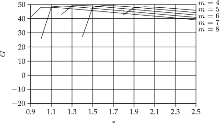
In Figures 9 and 10, we demonstrate the net busi-ness gain G in one unit of time as a function of
0.9 1.1 1.3 1.5 1.7 1.9 2.1 2.3 2.5 s −20 −10 0 10 20 30 40 50 G ... ... ... ... ... ... ... ... ... ... ... ... ... ...... ... ... ...... m= 4 m= 5 m= 6 m= 7 m= 8
Fig. 9. Net business gainGvs. s andm (idle-speed model). 0.9 1.1 1.3 1.5 1.7 1.9 2.1 2.3 2.5 s −20 −10 0 10 20 30 40 50 G ...... ... ... ... ... ... ...... ...... ...... ... ...... ...... ...... ... ... ... ... ... ...... ...... ...... ...... ...... ... ... ... ...... ...... ...... ...... ...... ...... ... m= 4 m= 5 m= 6 m= 7 m= 8
Fig. 10. Net business gain Gvs. sand m (constant-speed model).
s and m for the two power consumption models respectively, using the same parameters in Figures 1– 8, whereλ= 6.9. Form= 4,5,6,7,8, we displayGfor
s large enough such thatρ <1. Using our analytical results, we can findmandssuch that∂G/∂m= 0and
∂G/∂s= 0. For the idle-speed model, the theoretically optimal values are m = 5.56827 and s = 1.46819, which result in the maximum G= 49.25361 by using the closed-form approximation ofC. Practically,mcan be either 5 or 6. Whenm= 5, the optimal value ofsis 1.62236, which results in the maximumG= 49.16510. Whenm= 6, the optimal value ofsis 1.37044, which results in the maximum G = 49.18888. Hence, the practically optimal setting is m= 6and s= 1.37044, and the maximum net business gain in one unit of time is G = 49.29273 by using the exact expression of C. For the constant-speed model, the theoretically optimal values are m = 5.79074 and s = 1.35667, which result in the maximum G= 47.80769 by using the closed-form approximation ofC. Practically,mcan be either 5 or 6. Whenm= 5, the optimal value ofsis 1.55839, which results in the maximumG= 47.63979. Whenm= 6, the optimal value ofsis 1.31213, which results in the maximum G = 47.78640. Hence, the practically optimal setting is m= 6and s= 1.31213, and the maximum net business gain in one unit of time isG= 47.91830by using the exact expression of
C.
8
SIMULATION
RESULTS
Simulations have been conducted for two purposes, namely, (1) to validate our analytical results (Theo-rems 1 and 2); (2) and to find more effective queueing disciplines which increase the net profit of a service provider.
In Table 1, we show our simulation results by using the same parameters in Figures 1–10. For each
λ = 6.05,6.15, ...,6.95, we trace the behavior of an M/M/m queueing system with the FCFS queueing discipline by generating a Poisson stream of service requests with arrival rateλ, recording the waiting and response times of each service request, and calculat-ing the service charge to each service request. The average service charge of 1,000,000 service requests is reported in Table 1 for each λ. Notice that the maximum 99% confidence interval of all the data in the table is ±0.5165372%. The analytical data in the table are obtained by Theorem 2 to calculate the expected charge to a service request. It is easily observed that our simulation results match with the analytical data very well. These results validate our theoretically predicted service charge in Theorem 2, which is based on our analytical result on waiting time distribution in Theorem 1.
Our analysis in this paper is based on the FCFS queueing discipline. A different queueing discipline may change the distribution of the waiting times, and thus, changes the average task response time and the expected service charge. Since the cost of a service provider remains the same, an increased/decreased expected service charge to a service request in-creases/decreases the expected net business gain of a service provider. To show the effect of queueing disciplines on the net profit of a service provider, we only need to show the effect of queueing disciplines on the expected service charge to a service request. We consider two simple queueing disciplines, namely,
• Shortest Task First (STF): Tasks (service requests) are arranged in a waiting queue in the increasing order of their task execution requirements; • Largest Task First (LTF): Tasks (service requests)
are arranged in a waiting queue in the decreasing order of their task execution requirements. While other queueing disciplines can also be consid-ered, these two disciplines are already very encourag-ing.
In Table 1, we also display our simulation results for STF and LTF by using the same parameters for FCFS. For eachλ= 6.05,6.15, ...,6.95, we trace the behavior of an M/M/m queueing system with the STF and the LTF queueing disciplines respectively. The average service charge of 1,000,000 service requests is reported in Table 1 for eachλ. We have the following observa-tions.
Table 1: Simulation Results on the Expected Service Charge. λ Analytical FCFS STF LTF 6.05 9.8245499 9.8185300 9.9792709 9.5841297 6.15 9.7798220 9.7762701 9.9651989 9.5239829 6.25 9.7193304 9.7151778 9.9565597 9.4591742 6.35 9.6351404 9.6384268 9.9514632 9.3984495 6.45 9.5136508 9.5015511 9.9015669 9.3375343 6.55 9.3298719 9.3432460 9.8674891 9.2532065 6.65 9.0334251 9.0317035 9.8038810 9.1751988 6.75 8.5084481 8.4933564 9.7186839 9.0780185 6.85 7.4277447 7.4383065 9.5750764 8.9842690 6.95 4.4400583 4.4744746 9.3974538 8.8743559
• STF performs consistently better than FCFS. Furthermore, while the expected service charge drops significantly for FCFS when λ is close to the saturation point and the average waiting time becomes very long, the expected service charge of STF is still close toar¯when λis large.
• LTF performs worse than FCFS when λ is not very large. However, when λ is close to the saturation point, LTF performs better than FCFS in the sense that the expected service charge of LTF does not drop significantly when λis large. Unfortunately, due to lack of an analytical result on waiting time distribution similar to Theorem 1 for STF and LTF, the analytical work conducted in this paper for FCFS cannot be duplicated for STF and LTF. This can be an interesting subject for further investigation.
9
C
ONCLUDINGR
EMARKSWe have proposed a pricing model for cloud com-puting which takes many factors into considerations, such as the requirement rof a service, the workload
λ of an application environment, the configuration (m and s) of a multiserver system, the service level agreementc, the satisfaction (rands0) of a consumer, the quality (W andT) of a service, the penaltydof a low quality service, the cost (β andm) of renting, the cost (α,γ,P∗, andP) of energy consumption, and a service provider’s margin and profit a. By using an M/M/m queueing model, we formulated and solved the problem of optimal multiserver configuration for profit maximization in a cloud computing environ-ment. Our discussion can be easily extended to other service charge functions. Our methodology can be applied to other pricing models.
Our investigation in this paper is only an initial attempt in this area. We would like to mention several further research directions.
• First, in a cloud computing environment, a mul-tiserver system can be dynamically configured as a virtual cluster from a physical cluster, or a virtual multicore server from a physical multi-core processor, or a virtual multiserver system from any elastic and dynamic resources. Our profit maximization problem can be extended to
such virtual multiserver systems. To this end, a queueing model that accurately describes such a virtual multiserver system is required and needs to be developed. Such a model should be able to characterize a virtual multiserver system from a partially available physical system with deter-ministic or randomized availability.
• Second, our profit maximization problem can be extended to multiple heterogeneous multiserver systems of different sizes and speeds and applica-tion environments with total power consumpapplica-tion constraint. This is a multi-variable optimization problem, which is much more complicated than the optimization performed for a single multi-server system in this paper. Such optimization has significant and practical applications in de-signing energy-efficient data centers.
• Third, when a multicore server processor is spa-tially divided into several multicore servers, our profit maximization problem can be defined for multiple multiserver systems. When the cores have a fixed speed, the optimization problem has a total server size constraint. When the cores have variable speeds, the optimization problem has a total server size constraint as well as a power consumption constraint.
• Fourth, when a physical machine is temporally partitioned into several virtual machines, i.e., when we are facing a dynamic cloud configura-tion with multi-tenant utilizaconfigura-tion, our profit max-imization problem might be defined for multiple multiserver systems with total server speed con-straint. Again, this part of the research relies on an accurate queueing model for virtual machines which is currently not available.
We believe that the effort made in this paper should inspire significant subsequent studies in profit maxi-mization for cloud computing.
APPENDIX. PROOFS OF THE
THEOREMS
Proof of Theorem 1. If there are k < m tasks in the queueing system when a new service request arrives, the waiting time of the service request isWk = 0. The pdf ofWk can be represented as
fWk(t) =u(t),
for all0≤k≤m−1. Furthermore, we have
Wk = lim z→∞
1 2z = 0,
for all0≤k≤m−1.
If there are k ≥ m tasks in the queueing system when a new service request arrives, then the service request must wait until a server is available. Notice that due to the memoryless property of an exponential distribution, the remaining execution time of a task is always the same random variable as before, i.e.,
the original task execution time x with pdf fx(t) =
µe−µt,no matter how long the task has been executed. Let x1, x2, ..., xm be the remaining execution times of themtasks in execution when a new service request arrives. Then, we havefxj(t) =µe
−µt, for all1≤j≤
m.
It is clear that y = min{x1, x2, ..., xm} is the time until the next completion of a task. Since
P[y≥t] = m Y j=1 P[xj ≥t] = m Y j=1 e−µt=e−mµt, we get Fy(t) =P[y≤t] = 1−P[y≥t] = 1−e−mµt,
andfy(t) =mµe−mµt,that is,y is also an exponential random variable with mean1/mµ. The time until the next completion of a task is always the same random variable y, i.e., the minimum value of m i.i.d. expo-nential random variables with pdf fy(t) =mµe−mµt.
Notice that due to multiple servers, a task does not need to wait until all tasks in front of it are completed. Actually, the waiting time Wk of a task (under the condition that there are k≥m tasks in the queueing system when the task arrives) isWk =y1+y2+· · ·+
yk−m+1, wherey1, y2, ..., yk−m+1 are i.i.d. exponential random variables with the same pdffy(t) =mµe−mµt. The reason is that afterk−m+ 1completions of task executions, a task is at the front of the waiting queue and there is an available server, and the task will be scheduled to be executed. It is well known thaty1+
y2+· · ·+yk has an Erlang distribution whose pdf is
mµ(mµt)k−1 (k−1)! e
−mµt. Hence, we get the pdf ofWk
fWk(t) =
mµ(mµt)k−m (k−m)! e
−mµt, for all k≥m. Notice thaty¯= 1/mµand
Wk = (k−m+ 1)¯y= k−m+ 1 mµ = (k−m+ 1) ¯ x m, for all k≥m.
Summarizing the above discussion, we obtain the pdf of the waiting time W of a service request as follows: fW(t) = ∞ X k=0 pkfWk(t) = m−1 X k=0 pk ! u(t) + ∞ X k=m pk mµ(mµt)k−m (k−m)! e −mµt = (1−Pq)u(t) + ∞ X k=m p0 mmρk m! · mµ(mµt)k−m (k−m)! e −mµt = (1−Pq)u(t) +p0 mmρm m! mµe −mµt ∞ X k=m ρk−m(mµt)k−m (k−m)! = (1−Pq)u(t) +p0 (mρ)m m! mµe −mµt ∞ X k=0 (ρmµt)k k! = (1−Pq)u(t) +pmmµe−mµteρmµt = (1−Pq)u(t) +mµpme−(1−ρ)mµt. This proves the theorem.
Proof of Theorem 2. Since W is a random variable,
C(r, W), which is viewed as a function of W for a fixedr, is also a random variable. The expected charge to a service request with execution requirement r is (in the following, dt in parenthesis is the product of the penalty factor and the time variable)
C(r) =C(r, W) = Z ∞ 0 fW(t)C(r, t)dt = Z (a/d+c/s0−1/s)r 0 fW(t)C(r, t)dt = Z (a/d+c/s0−1/s)r 0 ((1−Pq)u(t) +mµpme−(1−ρ)mµt)C(r, t)dt = Z (a/d+c/s0−1/s)r 0 (1−Pq)u(t)C(r, t)dt + Z (a/d+c/s0−1/s)r 0 mµpme−(1−ρ)mµtC(r, t)dt = (1−Pq)ar+ Z (c/s0−1/s)r 0 mµpme−(1−ρ)mµtC(r, t)dt + Z (a/d+c/s0−1/s)r (c/s0−1/s)r mµpme−(1−ρ)mµtC(r, t)dt = (1−Pq)ar+ Z (c/s0−1/s)r 0 mµpme−(1−ρ)mµtardt + Z (a/d+c/s0−1/s)r (c/s0−1/s)r mµpme−(1−ρ)mµt a+cd s0 −d s r−dt dt = (1−Pq)ar+mµpmar Z (c/s0−1/s)r 0 e−(1−ρ)mµtdt +mµpm Z (a/d+c/s0−1/s)r (c/s0−1/s)r e−(1−ρ)mµt a+cd s0 −d s r−dt dt = (1−Pq)ar+mµpmar Z (c/s0−1/s)r 0 e−(1−ρ)mµtdt +mµpm a+cd s0 −d s r Z (a/d+c/s0−1/s)r (c/s0−1/s)r e−(1−ρ)mµtdt −dmµpm Z (a/d+c/s0−1/s)r (c/s0−1/s)r te−(1−ρ)mµtdt.
To continue the calculation, we notice that Z ebtdt= e bt b , and Z tebt= 1 b t−1 b ebt. Hence, we have Z (c/s0−1/s)r 0 e−(1−ρ)mµtdt = −e −(1−ρ)mµt (1−ρ)mµ (c/s0−1/s)r 0 = 1−e −(1−ρ)mµ(c/s0−1/s)r (1−ρ)mµ , and Z (a/d+c/s0−1/s)r (c/s0−1/s)r e−(1−ρ)mµtdt =−e −(1−ρ)mµt (1−ρ)mµ (a/d+c/s0−1/s)r (c/s0−1/s)r =e −(1−ρ)mµ(c/s0−1/s)r−e−(1−ρ)mµ(a/d+c/s0−1/s)r (1−ρ)mµ , and Z (a/d+c/s0−1/s)r (c/s0−1/s)r te−(1−ρ)mµtdt =− 1 (1−ρ)mµ t+ 1 (1−ρ)mµ e−(1−ρ)mµt (a/d+c/s0−1/s)r (c/s0−1/s)r = 1 (1−ρ)mµ c s0 −1 s r+ 1 (1−ρ)mµ e−(1−ρ)mµ(c/s0−1/s)r − a d+ c s0 −1 s r+ 1 (1−ρ)mµ e−(1−ρ)mµ(a/d+c/s0−1/s)r ! .
Based on the above results, we get
C(r) = (1−Pq)ar+mµpmar 1−e−(1−ρ)mµ(c/s0−1/s)r (1−ρ)mµ +mµpm a+cd s0 −d s r e−(1−ρ)mµ(c/s0−1/s)r−e−(1−ρ)mµ(a/d+c/s0−1/s)r (1−ρ)mµ −dmµpm 1 (1−ρ)mµ c s0 −1 s r+ 1 (1−ρ)mµ e−(1−ρ)mµ(c/s0−1/s)r − a d+ c s0 −1 s r+ 1 (1−ρ)mµ e−(1−ρ)mµ(a/d+c/s0−1/s)r ! = (1−Pq)ar+ apm 1−ρ r−re−(1−ρ)mµ(c/s0−1/s)r + pm 1−ρ a+cd s0 −d s re−(1−ρ)mµ(c/s0−1/s)r−re−(1−ρ)mµ(a/d+c/s0−1/s)r −dpm 1−ρ c s0 −1 s re−(1−ρ)mµ(c/s0−1/s)r + 1 (1−ρ)mµe −(1−ρ)mµ(c/s0−1/s)r − a d+ c s0 −1 s re−(1−ρ)mµ(a/d+c/s0−1/s)r − 1 (1−ρ)mµe −(1−ρ)mµ(a/d+c/s0−1/s)r ! = (1−Pq)ar+aPq r−re−(1−ρ)mµ(c/s0−1/s)r +Pq a+cd s0 −d s re−(1−ρ)mµ(c/s0−1/s)r−re−(1−ρ)mµ(a/d+c/s0−1/s)r −dPq c s0 −1 s re−(1−ρ)mµ(c/s0−1/s)r + 1 (1−ρ)mµe −(1−ρ)mµ(c/s0−1/s)r − a d+ c s0 −1 s re−(1−ρ)mµ(a/d+c/s0−1/s)r − 1 (1−ρ)mµe −(1−ρ)mµ(a/d+c/s0−1/s)r ! =ar− dPq (1−ρ)mµ e−(1−ρ)mµ(c/s0−1/s)r−e−(1−ρ)mµ(a/d+c/s0−1/s)r.
Sinceris a random variable,C(r), which is viewed as a function ofr, is also a random variable. Let the pdf of task execution requirementrto be
fr(z) =1 ¯
re
−z/¯r.
The expected charge to a service request is
C =C(r) = Z ∞ 0 fr(z)C(z)dz = Z ∞ 0 1 ¯ re −z/r¯C(z)dz = 1 ¯ r Z ∞ 0 e−z/r¯ az− dPq (1−ρ)mµ e−(1−ρ)mµ(c/s0−1/s)z −e−(1−ρ)mµ(a/d+c/s0−1/s)z ! dz
=1 ¯ r a Z ∞ 0 ze−z/r¯dz − dPq (1−ρ)mµ Z ∞ 0 e−((1−ρ)mµ(c/s0−1/s)+1/¯r)zdz − Z ∞ 0 e−((1−ρ)mµ(a/d+c/s0−1/s)+1/r¯)zdz ! . Since Z ∞ 0 ze−bzdz=−1 b z+1 b e−bz ∞ 0 = 1 b2, and Z ∞ 0 e−bzdz=−e −bz b ∞ 0 = 1 b, we get C =1 ¯ r ar¯ 2 − dPq (1−ρ)mµ 1 (1−ρ)mµ(c/s0−1/s) + 1/r¯ − 1 (1−ρ)mµ(a/d+c/s0−1/s) + 1/r¯ !! =a¯r− dPq (1−ρ)mµ 1 ¯ r(1−ρ)mµ(c/s0−1/s) + 1 − 1 ¯ r(1−ρ)mµ(a/d+c/s0−1/s) + 1 ! =a¯r− dPq (1−ρ)mµ· ¯ r(1−ρ)mµ(a/d) (¯r(1−ρ)mµ(c/s0−1/s) + 1) × 1 (¯r(1−ρ)mµ(a/d+c/s0−1/s) + 1) =a¯r− a¯rPq (¯r(1−ρ)mµ(c/s0−1/s) + 1) × 1 (¯r(1−ρ)mµ(a/d+c/s0−1/s) + 1) =a¯r 1− Pq ((ms−λr¯)(c/s0−1/s) + 1) × 1 ((ms−λ¯r)(a/d+c/s0−1/s) + 1) .
The theorem is proven.
ACKNOWLEDGMENTS
This work is partially supported by Ministry of Sci-ence and Technology of China under National 973 Basic Research Grants No. 2011CB302805 and No. 2011CB302505, and National 863 High-tech Program Grant No. 2011AA040501.
R
EFERENCES[1] http://en.wikipedia.org/wiki/CMOS
[2] http://en.wikipedia.org/wiki/Service level agreement [3] M. Armbrust, et al., “Above the clouds: a Berkeley view of
cloud computing,” Technical Report No. UCB/EECS-2009-28, February 2009.
[4] R. Buyya, D. Abramson, J. Giddy, and H. Stockinger, “Eco-nomic models for resource management and scheduling in grid computing,” Concurrency and Computation: Practice and Experience, vol. 14, pp. 1507-1542, 2007.
[5] R. Buyya, C. S. Yeo, S. Venugopal, J. Broberg, and I. Brandic, “Cloud computing and emerging IT platforms: vision, hype, and reality for delivering computing as the 5th utility,”Future Generation Computer Systems, vol. 25, no. 6, pp. 599-616, 2009. [6] A. P. Chandrakasan, S. Sheng, and R. W. Brodersen, “Low-power CMOS digital design,”IEEE Journal on Solid-State Cir-cuits, vol. 27, no. 4, pp. 473-484, 1992.
[7] B. N. Chun and D. E. Culler, “User-centric performance analy-sis of market-based cluster batch schedulers,”Proceedings of the 2nd IEEE/ACM International Symposium on Cluster Computing and the Grid, 2002.
[8] D. Durkee, “Why cloud computing will never be free,” Com-munications of the ACM, vol. 53, no. 5, pp. 62-69, 2010. [9] K. Hwang, G. C. Fox, and J. J. Dongarra,Distributed and Cloud
Computing, Morgan Kaufmann, 2012.
[10] Intel,Enhanced Intel SpeedStep Technology for the Intel Pentium M Processor – White Paper, March 2004.
[11] D. E. Irwin, L. E. Grit, and J. S. Chase, “Balancing risk and reward in a market-based task service,”Proceedings of the 13th IEEE International Symposium on High Performance Distributed Computing, pp. 160-169, 2004.
[12] L. Kleinrock,Queueing Systems, Volume 1: Theory, John Wiley and Sons, New York, 1975.
[13] Y. C. Lee, C. Wang, A. Y. Zomaya, and B. B. Zhou, “Profit-driven service request scheduling in clouds,” Proceedings of the 10th IEEE/ACM International Conference on Cluster, Cloud and Grid Computing, pp. 15-24, 2010.
[14] K. Li, “Optimal load distribution for multiple heterogeneous blade servers in a cloud computing environment,”Proceedings of the 25th IEEE International Parallel and Distributed Processing Symposium Workshops(8th High-Performance Grid and Cloud Computing Workshop), pp. 943-952, Anchorage, Alaska, May 16-20, 2011.
[15] K. Li, “Optimal configuration of a multicore server processor for managing the power and performance tradeoff,”Journal of Supercomputing, DOI: 10.1007/s11227-011-0686-1, published online 28 September 2011.
[16] P. Mell and T. Grance, “The NIST definition of cloud comput-ing,” National Institute of Standards and Technology, 2009. http://csrc.nist.gov/groups/SNS/cloud-computing/ [17] F. I. Popovici and J. Wilkes, “Profitable services in an
uncer-tain world,”Proceedings of the 2005 ACM/IEEE Conference on Supercomputing, 2005.
[18] J. Sherwani, N. Ali, N. Lotia, Z. Hayat, and R. Buyya, “Libra: a computational economy-based job scheduling system for clusters,” Software – Practice and Experience, vol. 34, pp. 573-590, 2004.
[19] C. S. Yeo and R. Buyya, “A taxonomy of market-based resource management systems for utility-driven cluster computing,” Software – Practice and Experience, vol. 36, pp. 1381-1419, 2006. [20] B. Zhai, D. Blaauw, D. Sylvester, and K. Flautner, “Theoretical and practical limits of dynamic voltage scaling,”Proceedings of the 41st Design Automation Conference, pp. 868-873, 2004.
Junwei Caoreceived his Ph.D. in computer science from the Uni-versity of Warwick, Coventry, UK, in 2001. He received his bachelor and master degrees in control theories and engineering in 1996 and 1998, respectively, both from Tsinghua University, Beijing, China. He is currently a Professor and Vice Director, Research Institute of Information Technology, Tsinghua University, Beijing, China. He is also Director of Common Platform and Technology Division, Ts-inghua National Laboratory for Information Science and Technology. Before joining Tsinghua University in 2006, he was a research scientist at MIT LIGO Laboratory and NEC Laboratories Europe for about 5 years. He has published over 130 papers and cited by international scholars for over 2,200 times. He is the book editor ofCyberinfrastructure Technologies and Applications, published by
Nova Science in 2009. His research is focused on advanced com-puting technologies and applications. Dr. Cao is a senior member of the IEEE Computer Society and a member of the ACM and CCF.
Kai Hwangis a Professor of EE/CS at the University of Southern California. He also chairs the IV-endowed visiting chair professor group at Tsinghua University in China. He received the Ph.D. from University of California, Berkeley in 1972. He has published 8 books and over 218 scientific papers in computer architecture, parallel processing, distributed systems, cloud computing, network security, and Internet applications. His popular books have been adopted worldwide and translated into 4 foreign languages. His published papers have been cited more than 9,000 times. Dr. Hwang’s latest bookDistributed and Cloud Computing: from Parallel Processing to the Internet of Things(with G. Fox and J. Dongarra) was just pub-lished by Kaufmann in 2011. Dr. Hwang was awarded an IEEE Fellow grade in 1986, received the 2004 CFC Outstanding Achievement Award, and the Founders Award for his pioneering work in parallel processing from IEEE IPDPS in 2011. He has served as a founding Editor-in-Chief of theJournal of Parallel and Distributed Computing
for 28 years. He has delivered 34 keynote addresses on advanced computing systems and cutting-edge information technologies in major IEEE/ACM Conferences. Dr. Hwang has performed advisory, consulting and collaborative work for IBM, Intel, MIT Lincoln Lab, JPL at Caltech, ETL in Japan, ITRI in Taiwan, GMD in Germany, INRIA in France, and Chinese Academy of Sciences.
Keqin Liis a SUNY Distinguished Professor in computer science and an Intellectual Ventures endowed visiting chair professor at Tsinghua University, China. His research interests are mainly in design and analysis of algorithms, parallel and distributed comput-ing, and computer networking. He has contributed extensively to processor allocation and resource management; design and analysis of sequential/parallel, deterministic/probabilistic, and approximation algorithms; parallel and distributed computing systems performance analysis, prediction, and evaluation; job scheduling, task dispatching, and load balancing in heterogeneous distributed systems; dynamic tree embedding and randomized load distribution in static networks; parallel computing using optical interconnections; dynamic loca-tion management in wireless communicaloca-tion networks; routing and wavelength assignment in optical networks; energy-efficient power management and performance optimization. Dr. Li has published over 240 research publications and has received several Best Pa-per Awards for his highest quality work. He is currently on the editorial board of IEEE Transactions on Parallel and Distributed Systems,IEEE Transactions on Computers,Journal of Parallel and Distributed Computing,International Journal of Parallel, Emergent and Distributed Systems,International Journal of High Performance Computing and Networking, andOptimization Letters.
Albert Y. Zomayais currently the Chair Professor of High Perfor-mance Computing and Networking and Australian Research Council Professorial Fellow in the School of Information Technologies, The University of Sydney. He is also the Director of the Centre for Distributed and High Performance Computing which was established in late 2009. Professor Zomaya is the author/co-author of seven books, more than 400 papers, and the editor of nine books and 11 conference proceedings. He is the Editor-in-Chief of theIEEE Transactions on Computersand serves as an associate editor for 19 leading journals, such as, theIEEE Transactions on Parallel and Dis-tributed SystemsandJournal of Parallel and Distributed Computing. Professor Zomaya is the recipient of the Meritorious Service Award (in 2000) and the Golden Core Recognition (in 2006), both from the IEEE Computer Society. Also, he received the IEEE Technical Committee on Parallel Processing Outstanding Service Award and the IEEE Technical Committee on Scalable Computing Medal for Excellence in Scalable Computing, both in 2011. Dr. Zomaya is a Chartered Engineer, a Fellow of AAAS, IEEE, and IET (UK).