M
a
na
ge
m
e
nt
R
e
se
a
rc
h
a
nd
P
ra
ct
ic
e
V
ol
um
e
2
,
I
ss
ue
1
/
M
a
rc
h
2
0
1
0
APPLICATION OF FISHBONE DIAGRAM TO
DETERMINE THE RISK OF AN EVENT WITH
MULTIPLE CAUSES
Gheorghe ILIE
1, Carmen Nadia CIOCOIU
21 UTI Grup SRL, Soseaua Oltenitei no.107A, Bucharest, Romania, [email protected] 2 Academy of Economic Studies, Piata Romana, 6, Bucharest, Romania, [email protected]
Abstract
Fishbone diagram (also known as Ishikawa diagram) was created with the goal of identifying and grouping the causes which generate a quality problem. Gradually, the method has been used also to group in categories the causes of other types of problems which an organization confronts with. This made Fishbone diagram become a very useful instrument in risk identification stage. The article proposes to extend the applicability of the method by including in the analysis the probabilities and the impact which allow determining the risk score for each category of causes, but also, of the global risk. The practical application is realized to analyze the risk “loosing specialists”.
Keywords: Fishbone diagram, global risk, probability, impact.
1. Introduction
The Fishbone diagram (also called the Ishikawa diagram) is a tool for identifying the root causes of quality problems. It was named after Kaoru Ishikawa, a Japanese quality control statistician, the man who pioneered the use of this chart in the 1960's (Juran, 1999).
The Fishbone diagram is an analysis tool that provides a systematic way of looking at effects and the causes that create or contribute to those effects. Because of the function of the Fishbone diagram, it may be referred to as a cause-and-effect diagram (Watson, 2004).
Fishbone (Ishikawa) diagram mainly represents a model of suggestive presentation for the correlations between an event (effect) and its multiple happening causes. The structure provided by the diagram helps team members think in a very systematic way. Some of the benefits of constructing a Fishbone diagram are that it helps determine the root causes of a problem or quality characteristic using a structured approach, encourages group participation and utilizes group knowledge of the process, identifies areas where data should be collected for further study (Basic Tools for Process Improvement, 2009).
The design of the diagram looks much like the skeleton of a fish. The representation can be simple, through bevel line segments which lean on an horizontal axis, suggesting the distribution of the multiple causes and sub-causes which produce them, but it can also be completed with qualitative and quantitative appreciations,
M
a
na
ge
m
e
nt
R
e
se
a
rc
h
a
nd
P
ra
ct
ic
e
V
ol
um
e
2
,
I
ss
ue
1
/
M
a
rc
h
2
0
1
0
with names and coding of the risks which characterizes the causes and sub-causes, with elements which show their succession, but also with other different ways for risk treatment. The diagram can also be used to determine the risks of the causes and sub-causes of the effect, but also of its global risk (Ciocoiu, 2008). Usually, the analysis after Fishbone diagram continues with other representation and establishing treatment priorities methods.
2. EMENTING FISHBONE DIAGRAM
To implement Fishbone diagram is used the logic scheme in Figure 1.
A special attention must be given to problem identification and its risk formalization.
- are identified problems, symptoms,
consequences, risks
- interview and consulting techniques are
used
- damages dimensions
- chronological elements, events
- treatment priorities
- main causes are detailed
-
in Boards of Directors, conferences or
consultations
- the diagram’s acceptance is decided by
the top management through an official
document
FIGURE 1 - LOGIC SCHEME OF FISHBONE DIAGRAM IMPLEMENTATION (ILIE, 2009)
LOOSING SPECIALISTS (5) YES NO PROBLEM IDENTIFICATION PROBLEM FORMALIZATION
IDENTIFYING MAIN AND SECONDARY CAUSES
PRIORITY CRITERIAS ARE ESTABLISHED DIAGRAM ANALYSE IS IT ACCEPTED? COMPLETION OF FISHBONE DIAGRAM ACCEPTED DIAGRAM (7) (6) (4) (3) (2) (1)
M
a
na
ge
m
e
nt
R
e
se
a
rc
h
a
nd
P
ra
ct
ic
e
V
ol
um
e
2
,
I
ss
ue
1
/
M
a
rc
h
2
0
1
0
The problem itself must be a desired or non-desired event characterized by risk and which must be treated (decreased) or exploited (capitalized). For the problem solved using Fishbone diagram, it must fulfill the following conditions:
it must be characterized by risk (R = p ∗∗∗∗ I), meaning that the probability of occurrence and its impact can be determined;
it must be a management objective with operational valence;
the causes producing it must be characterized by probability, possibility or frequency of occurrence; in turn, main causes must be also considered as effects (secondary or of second order) and sub-causes, named side-effects and which represent the causes of the secondary effects, must fulfill the same conditions as the main causes;
there must not exist bijective correlations, meaning the effect must not turn into its cause, regardless the positioning on the diagram.
Identifying main and secondary causes and their formalization must fulfill the same conditions as the problem identification and formalization, plus the following:
a priority criteria or a certain sequence in time (chronology) or a certain probability, possibility or frequency of occurrence can be identified;
main causes may or may not have one or more secondary causes;
if the question, the belonging of these causes can be identified: endogenous to the system of which the effect characterized by risk belongs or exogenous to the system (belonging to the environment); the number of main and secondary causes must be reasonable, usually not over 7-9 for main causes and 2-3 for the secondary causes of a main cause;
main and secondary causes must be representative and should allow monitoring or even management (can be sustained or fined through measures);
names given must be representative and suggestive for the relation cause-effect, and at the same time it should be able to be characterized by risks which enroll in the cause’s relevance.
Completion, the analysis as representativeness and relevance and its diagram acceptancerepresent a team-work which needs to take into consideration the objectivity of the analysis, its phenomenological representativeness (of the process), localization inside the achievement and representation criteria, coding possibility and establishing the exogenous or endogenous membership of its elements (Ilie, 2009).
M
a
na
ge
m
e
nt
R
e
se
a
rc
h
a
nd
P
ra
ct
ic
e
V
ol
um
e
2
,
I
ss
ue
1
/
M
a
rc
h
2
0
1
0
A lopsided diagram can indicate an over-focus in one area, a lack of knowledge in other areas, or it can simply indicate that the causes are focused in the denser area. A sparse diagram may indicate a lack of general understanding of the problem or just a problem with few possible causes (Straker).
The repartition of the causes and sub-causes on the diagram must meet some relevance, membership or timeline criteria, but they can be put in any preference order or even random (Ciocoiu, 2008).
After accepting the diagram, which must be stated in a decisional document (decision, minute, agreement etc.), follows the risk analyze of the elements in the diagram and then to the establishment of a plan for treatment or risk operation of the components (causes) and of the risk (global) of the characterized event (the effect).
3. ANALYSIS OF “LOOSING SPECIALISTS” DIAGRAM
For the application presented in this paper was chosen as the problem the fact of “loosing specialists”, an undesirable event with negative connotations. The risk assigned to the studied event will be actually named “the risk of loosing specialists”.
This risk fulfills all conditions of analytical element of the process developed inside an organization, regardless of its profile, and must not be confused with lost specialist value number. The number of lost specialists represents a performance indicator and it can be taken into consideration when analyzing the process itself.
The difference between the risk of loosing specialists and the number of lost specialists (binding in a certain period of time: one year, during the functioning period of an organization, during a contract period etc.) is that the number of specialists represents a static performance element, while the risk represents the dynamic of the phenomenon through the probability distribution of the effect occurrence, but also the impact which this effect has on the organization or on the process it belongs to.
Usually, the number of lost specialists is expressed by an integer and represents the performance of an occurred event, while the risk of loosing specialist is expressed by a fractional number or as a percentage and means the possibility, probability or forecast of an event occurrence. There is the possibility for the risk to be expressed also on a scale from 0 to 5, but even if in this case it is an integer (1, 2, 3, 4 or 5) it represents only a scale convention, meaning a fractional number or a percentage (regarding5). There also exists the possibility for the number of lost specialists to be expressed as a fraction or percentages, meaning that from 100 specialists were lost 7, that is 0,07 or 7%, but also in this case, the difference between the number of lost specialists, as a still image, and the risk, as a probabilistic, dynamic event, remains relevant.
M
a
na
ge
m
e
nt
R
e
se
a
rc
h
a
nd
P
ra
ct
ic
e
V
ol
um
e
2
,
I
ss
ue
1
/
M
a
rc
h
2
0
1
0
FIGURE 2 - FISHBONE DIAGRAM FOR LOOSING SPECIALISTS
The diagram (Figure 2) ischaracterized by:
6 main causes (management, organization, location, market, professional horizon and benefits) and 11 secondary causes, two for five main causes and one for the sixth main cause (professional horizon);
the representation on the diagram axis was made in an order of relevance (or of intake), inferred at the first analyze; from the beginning of the axis until the end of it, the most important causes being situated at the beginning (management and market);
placement of the main causes in the upper zone (considered the left part of the axis) or the lower zone (considered the right part of the axis) of the diagram was made according to a some conditioning, meaning that by the management depends organization and, obviously, the quality of the location where the process develops, and the market has elements of competition or of direct influence over the professional horizon and the benefits (as requirement);
the same principle tried to be respected also for the secondary causes, in the sense that the most far away of the horizontal axis have superior relevance than those closer (conflict situations are less relevant in the process than lack of efficiency);
COMPETITIVENESS LOW SPECIALISTS BIG DEMAND FOR LACK OF EFFICIENCY COMMUNICATION INEFFECTIVE HIERARCHY EXCESSIVE DEPROFESSIO-NALIZATION CONDITIONS POOR PERIPHERAL AREA LACK OF INCENTIVES REDUCED SALARIES CONFLICT SITUATIONS LOOSING SPECIALISTS BENEFITS PROFESSIONAL HORIZON MARKET ORGANIZATION MANAGEMENT LOCATION
M
a
na
ge
m
e
nt
R
e
se
a
rc
h
a
nd
P
ra
ct
ic
e
V
ol
um
e
2
,
I
ss
ue
1
/
M
a
rc
h
2
0
1
0
choosing the names of the main and secondary causes was done watching that they represent the main causes relevant during the process (management, market, organization, location etc.), while for the secondary causes (deprofessionalization, low competitiveness, poor conditions etc.) was watched for them to be as close as possible on the image of the risk.
If it is chosen the repartition criteria of main causes according to the environment or process belonging, in the left side (up) of the axis are represented the five endogenous causes, and on the right side (down) only the market, the only exogenous cause. Also in this case, on the left side of the axis are represented main causes in an order of relevance, from management to location (Figure 5).
4. CAUSES CODIFICATION
Causes codification is important in the risk analysis process using Fishbone diagram because it allows an easier operation and representation of the causes.
Codification is based on several principles:
belonging to parts of the diagram (left or right);
internal or external cause distribution (endogenous or exogenous);
chronology or occurrence frequency (time sequence or density of causes occurrence);
group composition of the code so that it would be more representative (of letters for membership or distribution and of numbers for chronology or succession);
the possibility to change the codification, if during the analyze the initial codification criteria changes (for example: the codification was made according to membership, but during the analyze has become a priority the sequence or the distribution); changing the codification is not indicated to be done more than once and, binding, this change materializes in a table of equivalence in which causes, old and new codes are written for each one. The table of equivalence for codification changes is accompanied by explanatory notes regarding initial and final codification criteria and about its reasons to change.
The layout inside the table of equivalence is done in the established order for the final codification, but so that there won’t appear confusions (when the number of causes is bigger) the current number of the causes from the initial codification table is kept (Table 1).
TABLE 1 - TABLE OF CAUSES (FINAL CODIFICATION) Current
Issue CAUSE SUB-CAUSE
INITIAL CODE FINAL CODE Initial current issue 3 3.1 Professional horizont Deprofessionalization S3 S31 D2 D21 5 5.1
M
a
na
ge
m
e
nt
R
e
se
a
rc
h
a
nd
P
ra
ct
ic
e
V
ol
um
e
2
,
I
ss
ue
1
/
M
a
rc
h
2
0
1
0
In Figure 2 for the causes codification is used the table presented in Table 2.
TABLE 2 – TABLE OF CAUSES CODIFICATIONCurrent issue CAUSE SUB-CAUSE CODE
1 Management S1 1.1 Lack of efficiency S11 1.2 Conflict situations S12 2 Organization S2 2.1 Excessive hierarchy S21 2.2 Ineffective communication S22 3 Locations S3 3.1 Peripheral area S31 3.2 Poor conditions S32 4 Market D1
4.1 Big demand for specialists D11
4.2 Low competitiveness D12 5 Professional horizon D2 5.1 Deprofessionalization D21 6 Benefits D3 6.1 Reduced salary D31 6.2 Lack of incentives D32
5. DETERMINING GLOBAL RISK
Global risk of the effect is conditioned by the risk of producing main causes and represents the weighted sum of them.
In the example presented in this paper, the distribution of the six main causes, on the left and the right (up and down) of the horizontal axis, based on the criteria of determining two categories of causes: conditions for activity(management, organization and locations) and competition, perspective and payment (market, professional horizon and benefits).
In this case, loosing specialists risk formalization, Rg, represent the weighted sum of the risks from the categories distributed on the left side, Rs, and on the right side, Rd, which contribution at the global risk is weighted regarding with their conditioning to them:
M
a
na
ge
m
e
nt
R
e
se
a
rc
h
a
nd
P
ra
ct
ic
e
V
ol
um
e
2
,
I
ss
ue
1
/
M
a
rc
h
2
0
1
0
Rg = ps
∗
∗
∗
∗
Rs
+ pd
∗
∗
∗
∗
Rd
,
where the sum of both categories weights must be equal to
1
(
ps + pd =1).
In turn, each category of risk is a weighted sum of the main causes of the risks distributed to the left
or to the right:
and Rs i are the main causes distributed to the left and
and Rdj are the main causes distributed to the right.
Also, each risk of a main cause represents the weighted sum of the risks of the secondary causes which determine its existence (the effect):
and Rsik represent the risk of the secondary causes which determine the existence of main causes to the left;
and Rdjl represent the risk of the secondary causes which determine the existence of main causes to the
right.
Determining the global risk unfolds according to the following algorithm based on tables or direct formalizations:
evaluate or determine risks of secondary causes (Rsik andpik; Rdjl andpjl), using any method
which can conduct to plausible results and, obviously, the appropriate formalization;
determine risks of main causes as weighted sums of the secondary causes risks and evaluate or are determine their weights inside the category they belong to (Rsi and pi; Rdjand pj);
determine risk categories by causes (Rs and Rd) and evaluate or determine their weights in the global risk (ps and pd);
determine the global risk (Rg) of the effect (event).
1,
p
;
Rs
p
Rs
n 1 i i n 1 i i i∗
∗
∗
∗
=
=
=
=
=
=
=
=
∑
∑
∑
∑
∑
∑
∑
∑
= = = = = = = =1,
p
;
Rd
p
Rd
m 1 j j m j j=
=
=
=
∗
∗
∗
∗
=
=
=
=
∑
∑
∑
∑
∑
∑
∑
∑
= == = = = = =1 j1,
p
;
Rs
p
Rs
k i, ik ik i ik=
=
=
=
∗
∗
∗
∗
=
=
=
=
∑
∑
∑
∑
∑
∑
∑
∑
k , i1,
p
;
Rd
p
Rd
l j, jl jl jl j=
=
=
=
∑
∑
∑
∑
∗
∗
∗
∗
∑
∑
∑
∑
=
=
=
=
l , jM
a
na
ge
m
e
nt
R
e
se
a
rc
h
a
nd
P
ra
ct
ic
e
V
ol
um
e
2
,
I
ss
ue
1
/
M
a
rc
h
2
0
1
0
We note that determining the weights can also be realized in another order than the one presented in the algorithm, taking in regard that weights are evaluated, are deducted or determined from other isomorphic tests or from events occurrence simulation.
For the accuracy of weights assessment, they are presented in a weights table or in a matrix (a map) of them (Table 3 and Table 4). Usually in this tables are not written the weights of cause’s categories.
TABLE 3 – TABLE OF MAIN AND SECONDARY CAUSES WEIGHTS
CODE CURRENT ISSUE MAIN CAUSES SECONDARY CAUSES WEIGHTS OF SECONDARY CAUSES WEIGHTS CONTROL WEIGHTS OF MAIN CAUSES WEIGHTS CONTROL 1 1.1. 1.2. S1 S11 S12 0,70 0,30 1 0,51 2 2.1. 2.2. S2 S21 S22 0,35 0,65 1 0,33 3 3.1. 3.2. S3 S31 S32 0,21 0,79 1 0,16 1 4 4.1. 4.2. D1 D11 D12 0,70 0,30 1 0,42 5 5.1. D2 D21 1 1 0,22 6 6.1. 6.2. D3 D31 D32 0,31 0,69 1 0,36 1
Causes settlement in the weights matrix represents another form of weights presentation, with the advantage of disclosure of direct relations between main and secondary causes.
Determining the global risk (in the case presently analyzed – the risk of loosing specialists) unfolds according to the following algorithm:
determine secondary risks causes (Rsik and Rdjl);
determine main risks causes (Rsi and Rdj);
determine categories risks by secondary causes (Rsand Rd); determine global risk(Rg).
M
a
na
ge
m
e
nt
R
e
se
a
rc
h
a
nd
P
ra
ct
ic
e
V
ol
um
e
2
,
I
ss
ue
1
/
M
a
rc
h
2
0
1
0
TABLE 4 – THE MATRIX OF MAIN, SECONDARY CAUSE WEIGHTS AND THEIR CATEGORIES MAIN CAUSES SECONDARY CAUSES/ CATEGORIES S1 S2 S3 D1 D2 D3 WEIGHTS CONTROL EFFECT WEIGHT S11 S12 0,70 0,30 Weight control 1 S21 S22 0,35 0,65 Weight control 1 S31 S32 0,21 0,79 Weight control 1 D11 D12 0,70 0,30 Weight control 1 D21 1 D31 D32 0,31 0,69 Weight control 1 Left side category S.
0,51 0,33 0,16 1 0,44 Right side category D
0,42 0,22 0,36 1 0,56
Weight control 1
Respecting the algorithm, to apply Fishbone diagram method in the case of loosing specialists, calculations are conducted as follows:
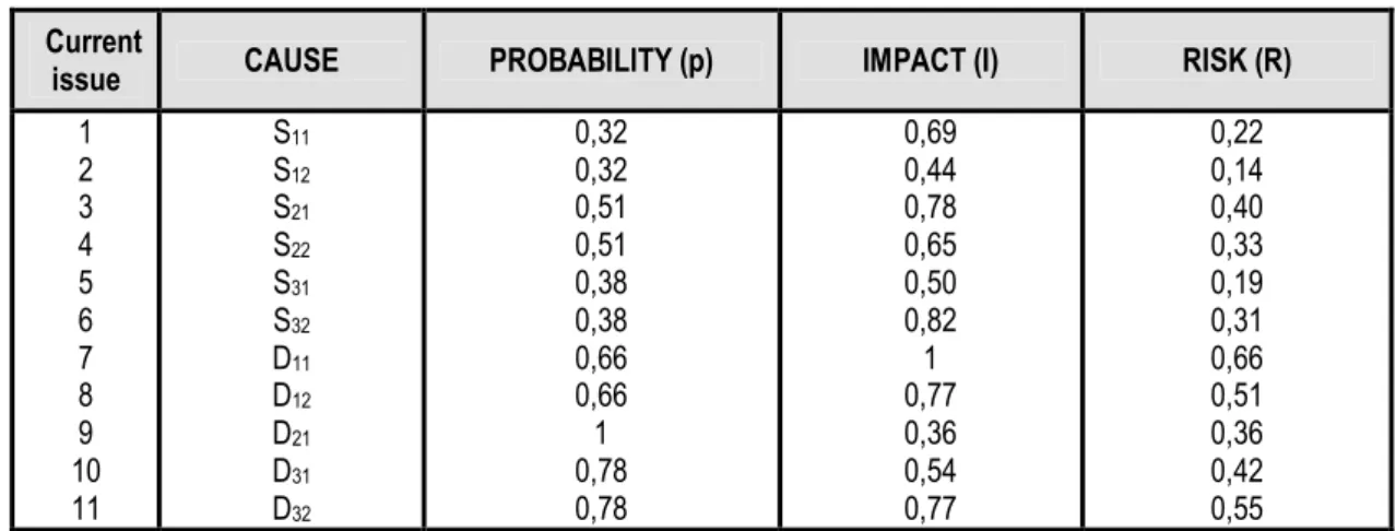
(I). Determining the risks of secondary causes basis on formalization (R = p∗∗∗∗I), according to which the risk (R) is equal to the product of multiplication between the event occurrence probability (p) and the impact (the consequences) of its occurrence (I).
The probabilities and the impact of the occurrence of this events are evaluated with different methods, presented in (Ciocoiu, 2008) and (Ilie, 2009), and are centralized in the table of probabilities and impact (consequences) of the secondary causes occurrence (Table 5).
M
a
na
ge
m
e
nt
R
e
se
a
rc
h
a
nd
P
ra
ct
ic
e
V
ol
um
e
2
,
I
ss
ue
1
/
M
a
rc
h
2
0
1
0
Taking into consideration the frequency of the secondary cause’s occurrence, their probabilities can be the same for the entire group of causes or the same for different groups or categories of causes. In what regards the impact is unlikely for them to be the same.
In the case presently analyzed were evaluated equal probabilities for the secondary causes which determine a main cause, while the impact was differently evaluated for each secondary cause.
TABLE 5 – TABLE OF SECONDARY CAUSES PROBABILITIES AND IMPACT Current
issue CAUSE PROBABILITY (p) IMPACT (I) RISK (R)
1 2 3 4 5 6 7 8 9 10 11 S11 S12 S21 S22 S31 S32 D11 D12 D21 D31 D32 0,32 0,32 0,51 0,51 0,38 0,38 0,66 0,66 1 0,78 0,78 0,69 0,44 0,78 0,65 0,50 0,82 1 0,77 0,36 0,54 0,77 0,22 0,14 0,40 0,33 0,19 0,31 0,66 0,51 0,36 0,42 0,55
(II). Determining the risks of main causes basis on the formalization of the relation between the risk of secondary causes and their weights in determining a main cause (Table 3 and Table 4).
In the case presently analyzed:
Rs1 = ps11∗∗∗∗ Rs11 ++++ ps12 ∗∗∗∗ Rs12 Rs2 = ps21∗∗∗∗ Rs21 ++++ ps22 ∗∗∗∗ Rs22 Rs3 = ps31∗∗∗∗ Rs31 ++++ ps32 ∗∗∗∗ Rs32 Rd1 = pd11∗∗∗∗ Rd11 ++++ pd12 ∗∗∗∗ Rd12 Rd2 = pd21∗∗∗∗ Rd21 Rd3 = pd31∗∗∗∗ Rd31 ++++ pd32 ∗∗∗∗ Rd32. So: Rs1 = 0,70 ∗∗∗∗ 0,22 ++++ 0,30 ∗∗∗∗ 0,14 = 0,16 ++++ 0,04 = 0,20 Rs2 = 0,35 ∗∗∗∗ 0,40 ++++ 0,65 ∗∗∗∗ 0,33 = 0,14 ++++ 0,22 = 0,36 Rs3 = 0,21 ∗∗∗∗ 0,19 ++++ 0,79 ∗∗∗∗ 0,31 = 0,04 ++++ 0,25 = 0,29 Rd1 = 0,70 ∗∗∗∗ 0,66 ++++ 0,30 ∗∗∗∗ 0,51 = 0,46 ++++ 0,15 = 0,61
M
a
na
ge
m
e
nt
R
e
se
a
rc
h
a
nd
P
ra
ct
ic
e
V
ol
um
e
2
,
I
ss
ue
1
/
M
a
rc
h
2
0
1
0
Rd2 = 1 ∗∗∗∗ 0,36 = 0,36 Rd3 = 0,31 ∗∗∗∗ 0,42++++ 0,69 ∗∗∗∗ 0,55 = 0,13 ++++ 0,38 = 0,51(III). Determining categories risks of secondary causes basis on the formalization of the weighted sum of the risks of secondary causes which belong to that category.
In the case presently analyzed:
Rs = p1∗∗∗∗ Rs1++++ p2∗∗∗∗ Rs2 ++++ p3 ∗∗∗∗ Rs3 Rd = p1∗∗∗∗ Rd1++++ p2∗∗∗∗ Rd2 ++++ p3 ∗∗∗∗ Rd3 So:
Rs = 0,51 ∗∗∗∗ 0,20 ++++ 0,33 ∗∗∗∗ 0,36 ++++ 0,16 ∗∗∗∗ 0,29 = 0,10 ++++ 0,12 ++++ 0,05 = 0,27
Rd = 0,42 ∗∗∗∗ 0,61 ++++ 0,22∗∗∗∗ 0,36 ++++ 0,36 ∗∗∗∗ 0,51 = 0,26 ++++ 0,08 ++++ 0,18 = 0,52.
(IV). Determining the global risk basis on the formalization of the weighted sum of the risks of the cause’s categories.
In the case presently analyzed:
Rg = 0,44 ∗∗∗∗ 0,27++++ 0,56∗∗∗∗ 0,52 = 0,12 ++++ 0,29 = 0,41.
6. INTERPRETATION OF RESULTS OBTAINED
On the risk scale with five levels (NEGLIGIBLE, MINOR, MEDIUM, MAJOR and DISASTER), the value 0,41
for the global risk of the effect loosing specialists situates it in the risk area MEDIUM (2,05 – equivalentfor the scale from 0 to 5). At the same time, the risks of main causes and of the categories of main causes frames the event characterized by risk in a vulnerability area described in the table presented in Table 6.
TABLE 6 – VULNERABILITIES TABLE CURRENT
ISSUE CAUSE CODE RISK VALUE RISK AREA
1 Management S1 0,20 (1) NEGLIGIBLE
2 Organization S2 0,36 (1,8) MINOR
3 Location S3 0,29 (1,45) MINOR
4 Market D1 0,61 (3,05) MAJOR
5 Professional horizon D2 0,36 (1,8) MINOR
6 Benefits D3 0,51(2,55) MEDIUM
7 Left Category S 0,27 (1,35) MINOR
M
a
na
ge
m
e
nt
R
e
se
a
rc
h
a
nd
P
ra
ct
ic
e
V
ol
um
e
2
,
I
ss
ue
1
/
M
a
rc
h
2
0
1
0
Counteracting the lost of specialists involves risk treatment measures taking into account the vulnerability of the organization to this threat (determined by the risk value) is MEDIUM, having MINOR vulnerability for the causes from the category of activity conditions (left) and MEDIUM for the causes from the category of environment and remuneration (left). In what regards secondary causes, the vulnerability of the organization to this is:
MAJOR to market action;
MEDIUM to the way of giving benefits;
MINOR to organization, location and professional horizon; NEGLIGIBLE to management quality.
Another way to interpret risk values is conditioned by the comparison of the values obtained with those established as an acceptance level.
Assuming that the acceptance level (Rp) for the risk of loosing specialists is of 0,30 (MINOR – 1,5), compare the value obtained for the global risk (0,41; 2,05 - MEDIUM) and if:
Rg <<<< Rp →→→→ the risk can be neglected and so does not require immediate treatment measures (for
improvement), and if Rg >>>> Rp →→→→ the risk must be treated (improved) through immediate measures. In the case presently analyzed,
Rg = 0,41 (2,05) >>>> Rp = 0,3 (1,5) and therefore treatment measures are required. TABLE 7 – TABLE OF TREATMENT CAUSES NECESSITY CURRENT
ISSUE CAUSE /CATEGORY SITUATION NECESSITY OF MEASURES
1 S1 0,20 < 0,30 NO 2 S2 0,36 > 0,30 YES 3 S3 0,29 < 0,30 NO 4 D1 0,61 > 0,30 YES 5 D2 0,36 > 0,30 YES 6 D3 0,51 > 0,30 YES 7 S 0,27 < 0,30 NO 8 D 0,52 > 0,30 YES
On a more complete analysis both the risk of the effect and the main causes (sometimes even the secondary ones) are compared against a risk of level and conclusions can be held regarding the repartition of treatment (improvement) measures for the risks on causes. Level risks can be equal with those of the global level risk or they can be different. To simplify the analysis consider the risk level of all secondary causes and of all risk
M
a
na
ge
m
e
nt
R
e
se
a
rc
h
a
nd
P
ra
ct
ic
e
V
ol
um
e
2
,
I
ss
ue
1
/
M
a
rc
h
2
0
1
0
categories is equal with that of the effect (0,3; 1,5). The conclusions of the analysis made regarding this level are presented in the table in Table7.
As the difference between the risk values determined and the level imposed is bigger, the intense the treatment (improvement) measures must be and applied as soon as possible.
The advantage of this kind of analysis is that in the absence of sufficient resources they can be concentrated in a different way on specific measures, and time horizons can be better established.
7. HIERARCHY OF CAUSES
For a more suggestive presentation of the cause contribution to the organization vulnerability, is used the model of their hierarchical (Ilie, 2009), by weighting towards the value of the main cause (the biggest value) and their representation on a suggestive graphic. To determine the hierarchy the table in Table 8is used.
TABLE 8 - TABLE OF CAUSES HIERARCHY CURRENT
ISSUE CAUSE SIZE HIERARCHY
1 S1 0,20 5 2 S2 0,36 3 3 S3 0,29 4 4 D1 0,61 1 5 D2 0,36 3 6 D3 0,51 2
For presentation causes weights are established according with the biggest risk value. In the case presently analyzed the biggest value is of 0,61, for which is chosen the measure of 10 units, and for the other causes the weight is determined multiplying their risk value with the weighting value (Mp), which equals to 10 and dividing it to the biggest risk value. For the case presently analyzed: Mp= 10 : 0,61= 16,4.
The table of weighted values of the risks for secondary causes is presented in Table 9. TABLE 9 – TABLE OF WEIGHTED VALUES
CURRENT
ISSUE CODE SIZE WEIGHTED VALUE
1 D1 0,61 10 2 D3 0,51 8,36 3 S2 0,36 5,90 4 D2 0,36 5,90 5 S3 0,29 4,76 6 S1 0,20 3,28
Based on the data from the table of weighted values the graphic of weighted distribution for secondary causes is realized in Figure 3.
M
a
na
ge
m
e
nt
R
e
se
a
rc
h
a
nd
P
ra
ct
ic
e
V
ol
um
e
2
,
I
ss
ue
1
/
M
a
rc
h
2
0
1
0
FIGURE 3 – GRAPHIC OF WEIGHTED DISTRIBUTION OF SECONDARY CAUSES
To become more suggestive and to take into account risk values determined for the causes, categories and effects (global risk), they are positioned on a modified Fishbone diagram, completed with risks sizes which characterize secondary causes and global risk (Figure 4).
FIGURE 4 – MODIFIED FISHBONE DIAGRAM
This type of diagram is suggestive because it places risks on the horizontal axis at their size, emphasizing, at the same time, the global risk and those on categories; that is why the modified diagram it is also called Fishbone risk diagram.
M
a
na
ge
m
e
nt
R
e
se
a
rc
h
a
nd
P
ra
ct
ic
e
V
ol
um
e
2
,
I
ss
ue
1
/
M
a
rc
h
2
0
1
0
The priority in risks treatment is usually established by the value size of risks for components, so that the first risks to be treated are those with bigger amplitude.
There are situations when treatment is realizes also in accordance with other criteria, for example: measure of frequency or of the impact.
Regardless of the chosen criteria for treatment, where resources are insufficient, treatment can be ranked with the help of PARETTO method (80/20), which establishes that treating 80% of the elements is important to solve one problem. The rest of 20% usually doesn’t change substantially the record.
For this thing, the risks of main causes are positioned in a table, starting with the one having the biggest risk value and the cumulative weight is calculated to determine the value of 80%, where treatment can be stopped
(Table 10).
TABLE 10 – TABLE OF PARETTO WEIGHTS CURRENT
ISSUE
CAUSE
CODE RISK VALUE WEIGHT
CUMULATIVE WEIGHT 1 D3 0,61 0,26 0,26 2 D1 0,51 0,22 0,48 3 D2 0,36 0,15 0,63 4 S2 0,36 0,15 0,78 5 S3 0,29 0,13 0,91 6 S1 0,20 0,09 1
The weight is calculated dividing the risk value of each cause to the cumulative value of the risks: 2,33. Following analysis on the table (choosing causes which frame the 80%), it is established that the first 4 causes will be treated with priority: D3, D1, D2 and S2. The other two causes will be treated only if there are
resources or at the time when resources are appropriately supplemented.
8. FISHBONE DIAGRAM STRUCTURED ACCORDING TO CAUSES AFFILIATION
To observe only the representation difference of Fishbone diagram we will analyze the same effect of “loosing specialists”, this time sharing the main causes according to their affiliation at the process and at the environment.
Main endogenous causes are those of management, organization, professional horizon, benefits and location (placed on the left side of the diagram axis), while the only exogenous cause is the market (placed on the right side) (Figure 5).
80% 20%
M
a
na
ge
m
e
nt
R
e
se
a
rc
h
a
nd
P
ra
ct
ic
e
V
ol
um
e
2
,
I
ss
ue
1
/
M
a
rc
h
2
0
1
0
FIGURE 5 – FISHBONE DIAGRAM STRUCTURED ACCORDING TO CAUSE AFFILIATION
The table of cause codification according to the new criteria is presented in Table 11. TABLE 11 – TABLE FOR CAUSE CODIFICATION ACCORDING TO THE NEW CRITERIA
CURRENT ISSUE CAUSE SUB-CAUSE CODE
1 Management S1 1.1 Lack of efficiency S11 1.2 Conflict situations S12 2 Organization S2 2.1 Excessive hierarchy S21 2.2 Ineffective communication S22 3 Professional horizon S3 3.1 Deprofessionalization S31 4. Benefits S4 4.1 Reduced salaries S41 4.2 Lack of incentives S42 5 Locations S5 5.1 Peripheral area S51 5.2 Poor conditions S52 6 Market D
6.1 Big demand of specialists D11
6.2 Low competitiveness D12 INCENTIVES AREA PROFESSIONAL HORIZON LACK OF SALARIES COMPETITIVENESS LOW SPECIALISTS BIG DEMAND FOR LACK OF EFFICIENCY COMMUNICATION INEFFECTIVE HIERARCHY EXCESSIVE DEPROFESSIO-NALIZATION CONDITIONS POOR PERIPHERAL REDUCED LOOSING SPECIALISTS MARKET CONFLICT SITUATIONS LOCATION
M
a
na
ge
m
e
nt
R
e
se
a
rc
h
a
nd
P
ra
ct
ic
e
V
ol
um
e
2
,
I
ss
ue
1
/
M
a
rc
h
2
0
1
0
After realizing the initial diagram structured after the affiliation of main causes and establishing their new codification, we pass on to determining the global risk complying with the same algorithm as in the first case.
Determining risks of secondary causes is realized with the same formalization R = p∗∗∗∗ I, the final results being shown in the probabilities, impact and risks of secondary causes table (Table 12). Because the same secondary causes were kept, regardless of the new positioning of the main causes, the risks determined for the secondary causes remain the same as in the previous case, obviously changing only their positioning inside the table.
TABLE 12 – TABLE OF RESTRUCTURED MAIN CAUSES PROBABILITIES AND IMPACT CURRENT
ISSUE CAUSE PROBABILITY IMPACT RISK
1 2 3 4 5 6 7 8 9 10 11 S11 S12 S21 S22 S31 S41 S42 S51 S52 D11 D12 0,32 0,32 0,51 0,51 1 0,78 0,78 0,38 0,38 0,66 0,66 0,69 0,44 0,78 0,65 0,36 0,54 0,71 0,50 0,82 1 0,77 0,22 0,14 0,40 0,33 0,36 0,42 0,55 0,19 0,31 0,66 0,51
Determining risks of main causes se realized in the same way as in the previous example, keeping the probabilities of the secondary causes and so:
Rs1= 0,70 ∗∗∗∗ 0,22 + 0,30 ∗∗∗∗ 0,14 = 0,22 Rs2= 0,35 ∗∗∗∗ 0,40 + 0,65 ∗∗∗∗ 0,33 = 0,36 Rs3=1 ∗∗∗∗ 0,36 = 0,36 Rs4= 0,31 ∗∗∗∗ 0,42 + 0,69 ∗∗∗∗ 0,55= 0,51 Rs5= 0,21 ∗∗∗∗ 0,19 + 0,79 ∗∗∗∗ 0,31 = 0,29 Rd=0,70∗∗∗∗ 0,66 + 0,30 ∗∗∗∗ 0,51= 0, 61
Determining risk categories of secondary risks is realized with the condition to change the weights of the main causes from the left side category, while the risk in the right side category will be equal to the risk of the main cause D.
M
a
na
ge
m
e
nt
R
e
se
a
rc
h
a
nd
P
ra
ct
ic
e
V
ol
um
e
2
,
I
ss
ue
1
/
M
a
rc
h
2
0
1
0
In such circumstances, according to the evaluation methods from the previous case, the weights of the secondary causes change and become: p1= 0,30; p2= 0, 26; p3= 0,20; p4= 0,13; p5= 0,11. And so the risk of
the category of main causes on the left is:
Rs = p1∗∗∗∗ Rs1 + p2 ∗∗∗∗ Rs2 + p3 ∗∗∗∗ Rs3 + p4 ∗∗∗∗ Rs4 + p5 ∗∗∗∗ Rs5 , where Σp1 + p2 + p3 + p4 + p5 = 1.
Rs = 0,30∗∗∗∗0,20 + 0,26∗∗∗∗0,36+ 0,20∗∗∗∗ 0,36 + 0,13∗∗∗∗0,51 + 0,11∗∗∗∗0,29 = 0,06 + 0,09 + 0,07 + 0,07 + 0,03 = 0,32
and Rd = 0,61.
Determining global risk is realized with the condition of keeping the weights of the cause categories, ps and pd,respectively 0,44 and 0,56.
Rg = 0,44 ∗∗∗∗ 0,32 + 0,56 ∗∗∗∗ 0,61 = 0,14 + 0,34 = 0,48.
With the new calculated values the diagram of risks distribution for main causes, categories of main causes and global risk is realized (Figure 6), according with the affiliation of main causes at the environment and process.
FIGURE 6 – FISHBONE DIAGRAM STRUCTURED AND MODIFIED
Comparing both modified diagrams (Figure 4 and Figure 6) the following conclusions can be drawn:
structuring according to the affiliation of main causes at the environment and process does not fundamentally change risks distribution because weights of the secondary causes and the categories of main causes were not changed;
M
a
na
ge
m
e
nt
R
e
se
a
rc
h
a
nd
P
ra
ct
ic
e
V
ol
um
e
2
,
I
ss
ue
1
/
M
a
rc
h
2
0
1
0
changing repartition density is normal and this will take to changing the structure of risks treatment measures;
there are other ways to restructure Fishbone diagram but solving the problem which means determining the global risk does not suffer substantial changes.
9. CONCLUSIONS
Fishbone diagram is a method used to determine the global risk of an event with multiple relevant causes, relatively easy to apply.
The application realized allows determining the risk of secondary and main causes, of cause’s categories and of the global risk, allows structuring of treatment measures on vulnerability areas, precisely oriented on the causes which determine high risk values.
Analysis of causes sequence can be a simple analyze which refers to the multitude of the causes and their sequence, but can be completed with other representation and hierarchy elements for risks treatment. Also, the method is used to simulate the dynamic of the process analyzed.
There are no instruments for risk analyze based exclusively on the Fishbone diagram. But there are instruments which include elements of primary or complementary analyze of this type.
The condition to successfully apply the method proposed here is a correct evaluation of the probabilities, weights and impact of the causes. As a result of this, the method is recommended especially for initial or comparative analyzes. Applying the method in relatively more simple cases is an excellent opportunity to understand the essence of risk analyze, of its bonds with establishing risk treatment measures and the dynamic evolution of risk values depending on the application of these methods.
REFERENCES
Basic Tools for Process Improvement. (1995, May 3). Retrived December 20, 2009, from Balanced Scorecard Institute: http://www.balancedscorecard.org/Portals/0/PDF/c-ediag.pdf
Ciocoiu, C. N. (2008). Managementul riscului. Teorii, practici, metodologii. Bucharest: ASE. Ilie, G. (2009). De la management la guvernare prin risc. Bucharest: UTI Press & Detectiv. Juran, J. M. (1999). Juran's Quality Handbook (5th Edition). McGraw-Hill.
Straker, D. (n.d.) Cause-Effect Diagram. Retrived January 10, 2010, from QualityTools: http://syque.com/quality_tools/toolbook/cause-effect/cause-effect.htm