On sequential estimation of a normal distribution having equal mean and variance

(1)

ON SEQUENTIAL ESTIMATION OF A NORMAL

DISTRIBUTION HAVING EQUAL MEAN AND VARIANCE

Saralees Nadarajah1

University of Manchester, Manchester M13 9PL, UK

Idika E. Okorie

University of Manchester, Manchester M13 9PL, UK

1. Introduction

The normal distribution with equal mean and variance arises in many applied ar-eas: collective theory of risk (Ammeter (1962)); contracts and supply assurance

in the UK health care market (Fennet al._{(1994)); estimation of individual}

asym-metry (Dongen (1999)); the effect of patenting on the networks and connections

of academic scientists (Fortiet al._{(2007)); gene expression data biclustering}

sta-bility (Badea and Tilivea (2008)); first passage percolation on random graphs

with finite mean degrees (Bhamidi et al. _{(2010)); postmortem body cooling}

(Kaliszan (2011)); detection of ADC clipping, quantization noise, and amplifier

saturation in surface electromyography (Fraseret al._{(2012)); rainfall frequency}

analysis (E. S. Chung (2013)); finding discriminatory genes (Khan and Greiner (2013)); impact of pacemaker failover configuration on mean time to recovery for small cloud clusters (Benz and Bohnert (2014)); interaction networks underlying the minority game (Caridi (2014)); to mention just a few.

This paper relates to one of the latest estimation problems for the normal

distribution with equal mean and variance. Let X1, X2, . . . , Xn be independent

and identically distributed observations from a normal distribution with both

the mean and variance equal to θ. Mukhopadhyay and Cicconetti (2004)

de-rived (among other things) the MLE and the UMVUE ofθ and discussed their

application to purely sequential and two-stage bounded risk estimation ofθ. The

MLE of θwas given by

b θ1n=

r Tn+1

4−

1

2, (1)

where

Tn= 1

n n X

i=1 Xi2.

(2)

The UMVUE of θwas given by

b

θ5n=b(u, n)n−1/2_I₍_{u, n}₎_, ₍₂₎

where

I(u, n) =

Z √

u

−√u

yexp √ny u−y2

(n−3)/2

dy, (3)

b(u, n) = √ 1

πΓ ((n−1)/2)q(u, n)

, (4)

q(u, n) =

∞

X

k=0

un/2+k−1_nk

22kΓ (n/2 +k)k! (5)

and

u=

n X

i=1 Xi2.

Mukhopadhyay and Cicconetti (2004) used the formulas given by the MLE (1) and the UMVUE (2) for purely sequential and two-stage bounded risk estimation

ofθ. Mukhopadhyay and Cicconetti (2004), however, encountered difficulties in

evaluating the UMVUE (2) and this limited the use of (2) as a sequential

esti-mator forθ. Mukhopadhyay and Cicconetti (2004) stated, for instance, that the

UMVUE (2) can be reduced to a “more closed form expression” and evaluated

“quickly and exactly” only whennis odd. Mukhopadhyay and Cicconetti (2004)

also stated that the complexity of the UMVUE (2) “increases asnincreases and

quickly renders computation” of the UMVUE (2) intractable. As far as we can see, much of the discussion in Mukhopadhyay and Cicconetti (2004) concern-ing the evaluation of the UMVUE (2) appears to be not correct, as shown in Sections 2 and 3. We feel that it is important that we point this out especially since Mukhopadhyay and Cicconetti Mukhopadhyay and Cicconetti (2004) has been cited by several other papers, see Mukhopadhyay (2006), Choi (2005), Kim

et al. _{(2007), Mukhopadhyay (2008), Mukhopadhyay and Bhattacharjee (2010),}

Bhattacharjee and Mukhopadhyay (2011) and S. Banerjee (2016).

The aim of this paper is two folded. Firstly, we derive a much simpler expression for the UMVUE (2). This expression turns out to be a ratio of two modified Bessel functions of the first kind, see Section 2. Secondly, using the derived formula, we compare the performance of the MLE (1) versus the

UMVUE (2) for purely sequential estimation ofθ, see Section 3.

Various special functions are used in Sections 2 and 3. Their definitions and detailed properties can be found in

http://functions.wolfram.com/Bessel-TypeFunctions/BesselI/,

http://functions.wolfram.com/Bessel-TypeFunctions/StruveL/,

http://functions.wolfram.com/HypergeometricFunctions/Hypergeometric0F1/,

http://functions.wolfram.com/HypergeometricFunctions/Hypergeometric1F1/.

(3)

2. Simpler expression for the UMVUE (2)

Here, we would like to show that the UMVUE (2) can be reduced in terms of a well known special function for any real numbern >1. Note that

I(u, n) =

( Z √_u

0

yexp √ny u₋y2(n−3)/2dy

− Z √_u

0

yexp −√ny u−y2(n−3)/2dy )

= 2 Z √_u

0

y u₋y2(n−3)/2sinh √nydy

= √πun/42n/2−1_n1/2−n/4_Γn−1

2

In/2

√

un, (6)

where the last step follows by equation (2.4.3.11) in Prudnikovet al.(1986) andIν(·)

denotes the modified Bessel function of the first kind of orderν defined by

Iν(x) =

∞

X

k=0

1 k!Γ (k+ν+ 1)

_x 2

2k+ν

. (7)

The equality in (6) holds for any real numbern >1. Using the definition in (7), one can expressq(u, n) in (5) as

q(u, n) =un/4−1/2_n1/2−n/4₂n/2−1_I n/2−1

√

un. (8)

Combining (2)-(4), (6) and (8), one obtains the simple form

b θ5n=

r u n

In/2

√ un In/2−1

√

un. (9)

The closed form expression in (9) is not only mathematically simpler than (2) which involves an infinite series and an integral. The closed form expression can also lead to more efficient computation of bθ5n in terms of computational time and computational

accuracy. In-built routines are usually based on efficient algorithms. The direct com-putation of infinite sums or integrals is usually not so efficient and can lead to round off errors.

There are many in-built routines for computing the modified Bessel function of the first kind. In the R software, it can be computed using besselI. In Maple, it can be computed usingBesselI. The following code in R was used for computing the UMVUE (9).

f=function (u,n) {

t1=besselI(sqrt(u*n),nu=(n/2),expon.scaled=TRUE) t2=besselI(sqrt(u*n),nu=((n/2)-1),expon.scaled=TRUE) tt=sqrt(u/n)*t1/t2

return(tt) }

(4)

0 20 40 60 80 100

1e−04

1e−02

1e+00

n

θ5n

0 20 40 60 80 100

1e−04

1e−02

1e+00

0 20 40 60 80 100

1e−04

1e−02

1e+00

0 20 40 60 80 100

1e−04

1e−02

1e+00

0 20 40 60 80 100

1e−04

1e−02

1e+00

0 20 40 60 80 100

1e−04

1e−02

1e+00

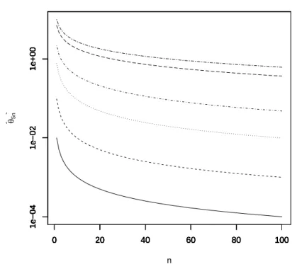
Figure 1 –θb5n versusnforu= 0.01 (solid line),u= 0.1 (dashed line),u= 1 (dotted

line),u= 5 (dotdash line),u= 50 (longdash line) andu= 100 (twodash line). They axis is in log scale.

To check the accuracy of the R code, we also computed the UMVUE (9) using BesselI in Maple. Maple like most other algebraic manipulation packages allows for arbitrary precision, so the accuracy of the values computed using Maple was not an issue. These values were plotted on the same axes of Figure 1. There appears to be no visual distinction between the values computed using Maple and R. Hence, the values computed using the R code can be considered accurate enough.

Mukhopadhyay and Cicconetti (2004) claimed that bθ5n can be computed much

more accurately for oddnand that the accuracy “also appears to be affected adversely whenuis either large or small”. But there is no evidence of this in Figure 1. According to this figure,bθ5n can be computed equally accurately for alln= 1,2, . . . ,100 and for

a range of values ofuincluding smalluand largeu.

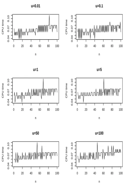
Mukhopadhyay and Cicconetti (2004) also claimed that θb5n “can be evaluated

quickly and exactly based on observed data only whennis odd” and the computational complexity ofθb5n“increases many fold asnincreases and quickly renders computation

of bθ5n” intractable. To verify this, we plotted the central processing unit time taken

for ten thousand computations of θb5nversusn= 1,2, . . . ,100 for a range of values of

(5)

0 20 40 60 80 100

0.04

0.07

0.10

u=0.01

n

CPU time

0 20 40 60 80 100

0.04

0.07

0.10

u=0.1

n

CPU time

0 20 40 60 80 100

0.04

0.07

0.10

u=1

n

CPU time

0 20 40 60 80 100

0.04

0.07

0.10

u=5

n

CPU time

0 20 40 60 80 100

0.04

0.07

0.10

u=50

n

CPU time

0 20 40 60 80 100

0.04

0.07

0.10

u=100

n

CPU time

Figure 2 – Central processing unit time taken to compute θb5n ten thousand times

(6)

It is well known thatIν(·) takes an elementary form ifνis a half integer. Actually,

ifν−1

2 is an integer then

Iν(z) = −

r 2 πzexp _πi 2 ₁

2−ν (

sinh _πi

2 ₁

2−ν

−z

· h2|ν|−1

4 i X

k=0

|ν|+2k−1 2

_!

(2k)! |ν_{| −}2k−1 2

!(2z)2k

+cosh πi 2 1 2−ν

−z

· h2|ν|−3

4 i X

k=0

|ν|+2k+1 2

! (2k+ 1)! |ν| −2k−3

2

_!(2z)₂_k₊₁ )

, (10)

where i =√−1 and [x] denotes the largest integer less than or equal tox. In particular,

I₋1/2(z) =

r 2 π cosh(z) √ z ,

I1/2(z) =

r 2 π sinh(z) √ z ,

I3/2(z) =

r 2 π

zcosh(z)−sinh(z) z3/2 ,

I5/2(z) =

r 2 π

z2+ 3sinh(z)−3zcosh(z)

z5/2 ,

and so on. So, the UMVUE (9) reduces to an elementary form if nis a positive odd integer.

Mukhopadhyay and Cicconetti (2004) also claimed thatbθ5n reduces to a

“closed-form expression solution for odd values ofn≥5”. Actually,θb5nreduces to a closed-form

expression for all odd values ofn_≥1. Forn= 1,3, the UMVUE (9) reduces to

b θ5n=

√

utanh √u

and

b θ5n=

1 √ 3

√

ucoth √u₋1,

respectively.

Equivalent representations for the UMVUE (9) in terms of other special functions are

b θ5n=

r u n

L₋n/2

√ un L1−n/2

√ un,

b θ5n=

u n

0F1

;n

2 + 1; un

4

0F1

;n 2; un 4 and b θ5n=

u n

1F1

n+ 1

2 ;n+ 1; 2 √

un

1F1

n₋1

2 ;n−1; 2 √

(7)

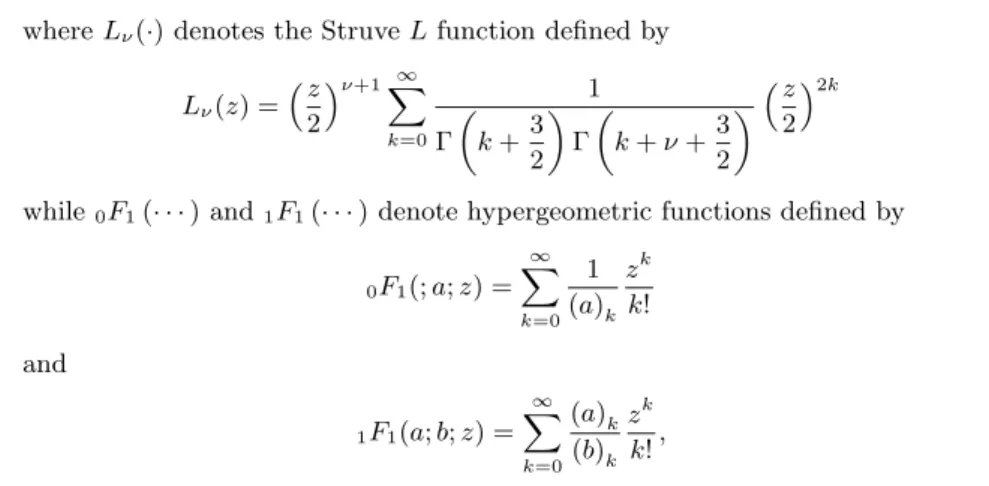
whereLν(·) denotes the StruveLfunction defined by

Lν(z) =

_z 2

ν+1_X∞

k=0

1

Γ

k+3 2

Γ

k+ν+3 2

z₂2k

while 0F1(· · ·) and1F1(· · ·) denote hypergeometric functions defined by

0F1(;a;z) =

∞

X

k=0

1 (a)_k

zk k!

and

1F1(a;b;z) =

∞

X

k=0

(a)_k (b)_k

zk k!,

respectively, where (e)k=e(e+ 1)· · ·(e+k−1) denotes the ascending factorial.

3. Sequential estimation of θ

Here, we compare the performance of the UMVUE (2) versus the MLE (1) for purely sequential estimation of θ. The MLE-based and the UMVUE-based sequential esti-mators of θ are given by (1) and (2), respectively, with the sample size ndefined by

the stopping rule: the smallest integern≥msuch thatn≥a∗_w−1₂b_θ2

1n

2θb1n+ 1

−1

, wherea∗_{is a constant and}_w_and_m_{are determined by the equations}

w= a

∗_2θ2

(2θ+ 1)n∗ (11)

and

m= 1 +

_a∗_2θ2 L

w(2θL+ 1)

, (12)

respectively, for givenn∗_,_θ_and_θ

L.

Mukhopadhyay and Cicconetti (2004) provided extensive tabulations of the sequen-tial estimators given by the MLE (1) and the UMVUE (2) for various combinations of n∗_, _θ _and _θ_L _with _a∗ _{= 1. For} _n∗ _{= 25 and}_n∗ _{= 35, Mukhopadhyay and}

Cic-conetti argued that the MLE (1) was the better estimator of the two. For the other values of n∗ _{considered, Mukhopadhyay and Cicconetti were unable to compute the}

UMVUE (2). Here, we provide a more comprehensive investigation of the relative performance of the MLE (1) versus the UMVUE (2) by using the derived formula (9). We computed 2,000 replications of both the MLE (1) and the UMVUE (9) for each of the following combinations: a∗_{= 1,} _n∗ _{= 25,}_50,_100,_200, _θ _{= 0.1,}_{0.2, . . . ,}_{1.5 and}

θL= 0.01θ,0.02θ, . . . ,0.99θ. For each set of 2,000 replications, we computed the risks

of estimation as

R1=a∗Eb

b θ1n−θ

2

and

R5=a∗Eb

b θ5n−θ

2

.

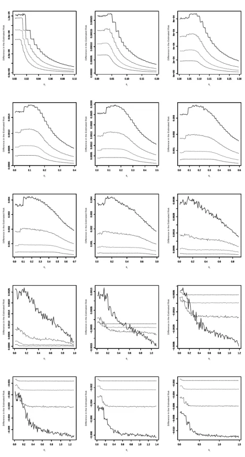
Figure 3 shows how the difference in the estimated risk,R1−R5, varies with respect

to θL for n∗ = 25,50,100,200 andθ = 0.1,0.2, . . . ,1.5. The following function in R

(8)

0.00 0.02 0.04 0.06 0.08 0.10 0.0e+00 4.0e−06 8.0e−06 1.2e−05 θL Diff

erence in the Estimated Risk

0.00 0.02 0.04 0.06 0.08 0.10

0.0e+00

4.0e−06

8.0e−06

1.2e−05

0.00 0.02 0.04 0.06 0.08 0.10

0.0e+00

4.0e−06

8.0e−06

1.2e−05

0.00 0.02 0.04 0.06 0.08 0.10

0.0e+00

4.0e−06

8.0e−06

1.2e−05

0.00 0.05 0.10 0.15 0.20

0.00000 0.00005 0.00010 0.00015 0.00020 θL Diff

0.00 0.05 0.10 0.15 0.20

0.00000

0.00005

0.00010

0.00015

0.00020

0.00 0.05 0.10 0.15 0.20

0.00000

0.00005

0.00010

0.00015

0.00020

0.00 0.05 0.10 0.15 0.20

0.00000

0.00005

0.00010

0.00015

0.00020

0.00 0.05 0.10 0.15 0.20 0.25 0.30

0e+00 2e−04 4e−04 6e−04 8e−04 θL Diff

0.00 0.05 0.10 0.15 0.20 0.25 0.30

0e+00

2e−04

4e−04

6e−04

8e−04

0.00 0.05 0.10 0.15 0.20 0.25 0.30

0e+00

2e−04

4e−04

6e−04

8e−04

0.00 0.05 0.10 0.15 0.20 0.25 0.30

0e+00

2e−04

4e−04

6e−04

8e−04

0.0 0.1 0.2 0.3 0.4

0.0000 0.0005 0.0010 0.0015 θL Diff

0.0 0.1 0.2 0.3 0.4

0.0000

0.0005

0.0010

0.0015

0.0 0.1 0.2 0.3 0.4

0.0000

0.0005

0.0010

0.0015

0.0 0.1 0.2 0.3 0.4

0.0000

0.0005

0.0010

0.0015

0.0 0.1 0.2 0.3 0.4 0.5

0.0005 0.0010 0.0015 0.0020 0.0025 0.0030 θL Diff

0.0 0.1 0.2 0.3 0.4 0.5

0.0005 0.0010 0.0015 0.0020 0.0025 0.0030

0.0 0.1 0.2 0.3 0.4 0.5

0.0005 0.0010 0.0015 0.0020 0.0025 0.0030

0.0 0.1 0.2 0.3 0.4 0.5

0.0005 0.0010 0.0015 0.0020 0.0025 0.0030

0.0 0.1 0.2 0.3 0.4 0.5 0.6

0.001

0.002

0.003

θL

Diff

0.0 0.1 0.2 0.3 0.4 0.5 0.6

0.001

0.002

0.003

0.0 0.1 0.2 0.3 0.4 0.5 0.6

0.001

0.002

0.003

0.0 0.1 0.2 0.3 0.4 0.5 0.6

0.001

0.002

0.003

0.0 0.1 0.2 0.3 0.4 0.5 0.6 0.7

0.001 0.002 0.003 0.004 θL Diff

0.0 0.1 0.2 0.3 0.4 0.5 0.6 0.7

0.001

0.002

0.003

0.004

0.0 0.1 0.2 0.3 0.4 0.5 0.6 0.7

0.001

0.002

0.003

0.004

0.0 0.1 0.2 0.3 0.4 0.5 0.6 0.7

0.001

0.002

0.003

0.004

0.0 0.2 0.4 0.6 0.8

0.001 0.002 0.003 0.004 θL Diff

0.0 0.2 0.4 0.6 0.8

0.001

0.002

0.003

0.004

0.0 0.2 0.4 0.6 0.8

0.001

0.002

0.003

0.004

0.0 0.2 0.4 0.6 0.8

0.001

0.002

0.003

0.004

0.0 0.2 0.4 0.6 0.8

0.0005 0.0015 0.0025 0.0035 θL Diff

0.0 0.2 0.4 0.6 0.8

0.0005

0.0015

0.0025

0.0035

0.0 0.2 0.4 0.6 0.8

0.0005

0.0015

0.0025

0.0035

0.0 0.2 0.4 0.6 0.8

0.0005

0.0015

0.0025

0.0035

0.0 0.2 0.4 0.6 0.8 1.0

0.0000 0.0005 0.0010 0.0015 0.0020 0.0025 θL Diff

0.0 0.2 0.4 0.6 0.8 1.0

0.0000 0.0005 0.0010 0.0015 0.0020 0.0025

0.0 0.2 0.4 0.6 0.8 1.0

0.0000 0.0005 0.0010 0.0015 0.0020 0.0025

0.0 0.2 0.4 0.6 0.8 1.0

0.0000 0.0005 0.0010 0.0015 0.0020 0.0025

0.0 0.2 0.4 0.6 0.8 1.0

−0.0015 −0.0005 0.0005 0.0015 θL Diff

0.0 0.2 0.4 0.6 0.8 1.0

−0.0015

−0.0005

0.0005

0.0015

0.0 0.2 0.4 0.6 0.8 1.0

−0.0015

−0.0005

0.0005

0.0015

0.0 0.2 0.4 0.6 0.8 1.0

−0.0015

−0.0005

0.0005

0.0015

0.0 0.2 0.4 0.6 0.8 1.0 1.2

−0.0035 −0.0025 −0.0015 −0.0005 θL Diff

0.0 0.2 0.4 0.6 0.8 1.0 1.2

−0.0035

−0.0025

−0.0015

−0.0005

0.0 0.2 0.4 0.6 0.8 1.0 1.2

−0.0035

−0.0025

−0.0015

−0.0005

0.0 0.2 0.4 0.6 0.8 1.0 1.2

−0.0035

−0.0025

−0.0015

−0.0005

0.0 0.2 0.4 0.6 0.8 1.0 1.2

−0.005 −0.004 −0.003 −0.002 −0.001 θL Diff

0.0 0.2 0.4 0.6 0.8 1.0 1.2

−0.005

−0.004

−0.003

−0.002

−0.001

0.0 0.2 0.4 0.6 0.8 1.0 1.2

−0.005

−0.004

−0.003

−0.002

−0.001

0.0 0.2 0.4 0.6 0.8 1.0 1.2

−0.005

−0.004

−0.003

−0.002

−0.001

0.0 0.2 0.4 0.6 0.8 1.0 1.2 1.4

−0.008 −0.006 −0.004 −0.002 θL Diff

0.0 0.2 0.4 0.6 0.8 1.0 1.2 1.4

−0.008

−0.006

−0.004

−0.002

0.0 0.2 0.4 0.6 0.8 1.0 1.2 1.4

−0.008

−0.006

−0.004

−0.002

0.0 0.2 0.4 0.6 0.8 1.0 1.2 1.4

−0.008

−0.006

−0.004

−0.002

0.0 0.5 1.0 1.5

−0.010 −0.008 −0.006 −0.004 −0.002 θL Diff

0.0 0.5 1.0 1.5

−0.010

−0.008

−0.006

−0.004

−0.002

0.0 0.5 1.0 1.5

−0.010

−0.008

−0.006

−0.004

−0.002

0.0 0.5 1.0 1.5

−0.010

−0.008

−0.006

−0.004

−0.002

Figure 3 – The difference in the estimated risk, R1 − R5, versus θL for θ =

0.1,0.2, . . . ,1.5,n∗_{= 25 (solid line),}_n∗_{= 50 (dashed line),}_n∗_{= 100 (dotted line) and}

(9)

ff=function (astar,nstar,theta,thetaL) {

tt=astar*2*theta**2*(2*theta+1)**(-1) w=tt/nstar

m=trunc(astar*(1/w)*2*thetaL**2*(2*thetaL+1)**(-1))+1 for (i in 1:2000)

{

x=rnorm(m,mean=theta,sd=theta**2) tn=mean(x**2)

theta1n=sqrt(tn+0.25)-0.5 n=m

repeat {

tt=astar*(1/w)*2*theta1n**2*(2*theta1n+1)**(-1) if (n>=tt) break

n=n+1

x=c(x,rnorm(1,mean=theta,sd=theta**2)) tn=mean(x**2)

theta1n=sqrt(tn+0.25)-0.5 }

theta1[i]=theta1n u=sum(x**2)

theta5[i]=sqrt(u/n)*besselI(sqrt(u*n),nu=n/2,expon.scaled=TRUE) /besselI(sqrt(u*n),nu=n/2-1,expon.scaled=TRUE)

}

ttt=astar*mean((theta1-theta)**2)-astar*mean((theta5-theta)**2) return(tt)

}

We can observe the following from Figure 3: the UMVUE is the better of the two estimators for θ ≤1; the UMVUE performs relatively better asθ increases to 1; the UMVUE performs relatively better asθLdecreases; the UMVUE performs relatively

better asn∗_{decreases; the MLE is the better of the two estimators for}_{θ >}_{1 and}_θ

Lnot

too small; the MLE performs relatively better asθ >1 increases; the MLE performs relatively better asθLincreases; the MLE performs relatively better asn∗decreases.

The estimates given in the tables in Mukhopadhyay and Cicconetti (2004) for n∗_{= 25,}_{35 do coincide with the estimates we obtained up to the decimal places given.}

The codes given in this paper can be used to compute the estimates to any decimal place.

4. Conclusions

Given a normal random variable with both mean and standard deviation equal to θ, we have derived a simple expression for the UMVUE ofθ. This is the simplest known to date, hence it can be applied efficiently to sequential problems involving the normal random variable.

We have compared the performances of the UMVUE and MLE in terms of risk. Some of the main findings are that the UMVUE is the better forθ≤1, the UMVUE performs relatively better asθ increases to 1, the MLE is the better forθ >1 and the MLE performs relatively better asθ >1 increases.

(10)

Acknowledgements

The authors would like to thank the Editor and the referee for careful reading and comments which improved the paper.

References

H. Ammeter(1962). Experience rating a new application of the collective theory of

risk. ASTIN Bulletin, 2, pp. 261–270.

L. Badea,D. Tilivea (2008). Nonnegative decompositions with resampling for

im-proving gene expression data biclustering stability. Proceedings of the 18th European Conference on Artificial Intelligence.

K. Benz,T. M. Bohnert(2014).Impact of pacemaker failover configuration on mean

time to recovery for small cloud clusters. Proceedings of the 7th IEEE International Conference on Cloud Computing, pp. 384–391.

S. Bhamidi,R. van der Hofstad,G. Hooghiemstra(2010). First passage

percola-tion on random graphs with finite mean degrees. Annals of Applied Probability, 20, pp. 1907–1965.

D. Bhattacharjee, N. Mukhopadhyay (2011). On mp test and the mvues in a

n(θ, cθ) distribution withθ unknown: Illustrations and applications. Journal of the Japan Statistical Society, 41, pp. 75–91.

I. Caridi (2014). Properties of interaction networks underlying the minority game.

Physical Review E, 90.

K. Choi (2005). Some properties of sequential point estimation of the mean. Journal

of Korean Data and Information Science Society, 16, pp. 657–663.

V. Dongen (1999). Unbiased estimation of individual asymmetry. Journal of

Evolu-tionary Biology, 13, pp. 107–112.

S. U. K. E. S. Chung(2013). Bayesian rainfall frequency analysis with extreme value

using the informative prior distribution. KSCE Journal of Civil Engineering, 17, pp. 1502–1514.

P. Fenn,N. Rickman,A. McGuire(1994). Contracts and supply assurance in the

uk health care market. Journal of Health Economics, 13, pp. 125–144.

E. Forti,C. Franzoni,M. Sobrero(2007). The effect of patenting on the networks

and connections of academic scientists. Working Paper.

G. D. Fraser,A. D. C. Chan,J. R. Green,D. MacIsaac(2012). Detection of adc

clipping, quantization noise, and amplifier saturation in surface electromyography. Proceedings of the IEEE International Symposium on Medical Measurements and Applications, pp. 1–5.

M. Kaliszan(2011). Does a draft really influence postmortem body cooling? Journal

of Forensic Sciences, 56, pp. 1310–1314.

S. Khan,R. Greiner(2013). Finding discriminatory genes: A methodology for

(11)

S. K. Kim, S. L. Kim, Y. W. Lee (2007). Sequential confidence intervals with β -protection in a normal distribution having equal mean and variance. Journal of Applied Mathematics and Computing, 23, pp. 479–488.

N. Mukhopadhyay(2006). Mvue for the mean with one observation. The American

Statistician, 60, pp. 71–74.

N. Mukhopadhyay,D. Bhattacharjee(2010). A note on minimum variance

un-biased estimation. Communications in Statistics—Theory and Methods, 39, pp. 1466–1476.

N. Mukhopadhyay,G. Cicconetti(2004). Applications of sequentially estimating

the mean in a normal distribution having equal mean and variance. Sequential Anal-ysis, 23, pp. 625–665.

B. M. d. S. N. Mukhopadhyay(2008).Theory and applications of a new methodology

for the random sequential probability ratio test. Statistical Methodology, 5, pp. 424– 453.

A. P. Prudnikov,Y. A. Brychkov, O. I. Marichev(1986). Integrals and Series,

volume 1. Gordon and Breach Science Publishers, Amsterdam.

R Development Core Team(2016).R: A Language and Environment for Statistical

Computing. Vienna, Austria.

N. M. S. Banerjee (2016). A general sequential fixed-accuracy confidence interval

estimation methodology for a positive parameter: Illustrations using health and safety data. Annals of the Institute of Statistical Mathematics, 68, pp. 541–570.

Summary

Mukhopadhyay and Cicconetti (2004) derived the Maximum Likelihood Estimator (MLE) and the Uniformly Minimum Variance Unbiased Estimator (UMVUE) of θ in N(θ, θ) and discussed their application to purely sequential and two-stage bounded risk estimation of θ. In this paper, a much simpler expression is derived for the UMVUE of θ. Using this expression, a comprehensive investigation is provided for comparing the performances of the sequential estimators based on the MLE and the UMVUE.