The Socio-demographic Structure of the First Wave of the TwinLife Panel Study: A Comparison with the Microcensus

(1)

The Socio-demographic Structure of the

First Wave of the TwinLife Panel Study:

A Comparison with the Microcensus

Volker Lang & Anita Kottwitz

Bielefeld University

Abstract

The TwinLife panel is the first longitudinal study of twin families in Germany based on a national probability sample. TwinLife has been developed to facilitate genetic sensitive research on social inequalities. The aim of this paper is to assess the usability of the Twin-Life sample for such research. Therefore, first, we analyze if the social background of twins living in Germany is adequately represented in the TwinLife sample; and second, we also investigate if there are socio-demographic differences between twin and other multiple-child households in Germany which would restrict the generalizability of findings based on the TwinLife study. Specifically, we compare the distributions of key socio-demographic indicators in TwinLife with the German Microcensus using a proxy-twin and a multiple-child household sample. Our analyses show that the TwinLife sample covers the full distri-butions of core social inequality indicators including the lower and upper bounds, enabling researchers to use TwinLife for detailed studies of the gene-environment interplay. Fur-thermore, we demonstrate that (proxy-)twin and other multiple-child households in Germa-ny are similar regarding most socio-demographic indicators. However, our analyses also indicate that participation in the first wave of the TwinLife panel was slightly selective with respect to parental education and German citizenship, especially in the younger cohorts of the study. We suggest a weighting scheme to address this selectivity.

Keywords: Twin Families, Multiple-Child Families, Family Demography, Sampling Design, Extended Twin Family Design, Germany

(2)

Acknowledgments

We like to thank two anonymous reviewers, Martin Diewald, and Kristina Krell for very helpful comments on an earlier version of this paper. The TwinLife project is funded by the German Research Foundation (DFG) (grant number 220286500) award-ed to Martin Diewald, Rainer Riemann, and Frank M. Spinath. The TwinLife study received ethical approval from the German Psychological Association (protocol num-bers: RR 11.2009 and RR 09.2013).

Direct correspondence to

Volker Lang, Bielefeld University, Department of Sociology, Project TwinLife, Postbox 100131, 33501 Bielefeld, Germany

E-mail: [email protected]

Studying twins reared together is a prominent research strategy to assess the influ-ence of genetic endowment on human development (Polderman et al., 2015). By comparing monozygotic twins – who are genetically (almost) identical – with dizy-gotic twins – who share about half of the genes that vary between humans (like ordinary siblings), it is possible to estimate the share of variance in an outcome attributable to (additive) genetic influences (Plomin et al., 2016).1_{Nevertheless,}

such estimates of genetic influences are by no means a fixed quantity but strongly dependent on the development stage (i.e., the age) of the twins (Haworth et al., 2010; Turkheimer, 2000) as well as on the environmental conditions in which a genetic potential is actualized (Shanahan & Hofer, 2005; Bronfenbrenner & Ceci, 1994). A central facet of these environmental conditions is the social background (Guo & Stearns, 2002). In consequence, studying the different forms in which genetic influ-ences depend on environments – so called gene-environment interactions and cor-relations – is a major focus of current behavior genetic research (Zavala et al. 2018; Tucker-Drob & Bates, 2016) as well as a topic of growing interest in the research on social inequalities (Selita & Kovas, 2019; Diewald et al., 2016; Nielsen, 2016).

However, twin samples covering a wide range of environmental conditions and development stages are needed to conduct studies on the influence of genes on social inequalities. The TwinLife panel – which is run in cooperation by research teams at Bielefeld University and Saarland University – was designed to facilitate such research and is the first longitudinal study of twin families in Germany based on a national probability sample (Mönkediek et al., 2019, Hahn et al., 2016). To assess the usability of the TwinLife sample for social stratified research on genetic influences, we address two research questions in this paper: first, is the social back-ground of twins living in Germany captured by the TwinLife sample to facilitate genetic sensitive analyses differentiated by social background? And second, is the

(3)

social background of twin households comparable to all multiple-child households in Germany in order to support the generalizability of social stratified analyses on genetic influences?

In contrast to many other countries (e.g., The Netherlands: Ligthart et al., 2019; Sweden: Zagai et al., 2019), no twin registry is available for Germany to answer these research questions. Alternatively, we compare the TwinLife sample with two selected samples based on the German Microcensus Survey conducted by the Federal Statistical Office (Destatis, 2014a, 2014b; Lengerer et al., 2007): a proxy-twin household sample and a multiple-child household sample. Specifically, we compare parental education, household income, parental citizenship status, the composition of the households, and the population sizes of the communities of resi-dence. In addition, we investigate maternal age at childbirth as a potential reason for differences in the distributions of these social background indicators. Thus, if the TwinLife sample is representative for twin families in Germany, we expect to see no relevant differences in the distributions of these social background indica-tors between the TwinLife and the Microcensus proxy-twin samples (hypothesis 1). Moreover, since the environmental conditions in which children are reared can systematically differ between twin and other types of multiple-child families, it can be questioned if results obtained by studying twins are generalizable to a whole population. In some cases – like the age gap between siblings – such differ-ences are undeniable. Regarding the distributions of social background indicators, differences between twin and other multiple-child families cannot be precluded. If the social backgrounds of twin and other multiple-child families in Germany are similar, we should not find any relevant differences in the distributions of the ana-lyzed indicators between the Microcensus proxy-twin and multiple-child samples (hypothesis 2).

(4)

Data and Methods

The TwinLife Panel Study

Study Design

The TwinLife study collects longitudinal data on families with monozygotic or dizygotic twin children. To exclude effects of within-twin-pair gender differences, the study includes only same-sex dizygotic twins. The base population of TwinLife consists of four birth cohorts of twins: the youngest twins, in cohort 1, were born in 2009 or 2010, the twins in cohort 2 in 2003 or 2004, the twins in cohort 3 in 1997 or 1998, and the oldest twins, in cohort 4, between 1990 and 1993. At the time of the first survey, these twins were aged around 5, 11, 17, and 23 to 24. Over the planned panel period, TwinLife covers important life course transitions ranging from school entry to the labor market entry phase, and also important life stages for meeting a partner and starting a family. The TwinLife surveys are conducted annually and survey modes alternate between face-to-face interviews at home and telephone interviews.

In addition, the TwinLife study combines this cohort-sequential design with an extended twin family design (ETFD). As part of the ETFD, the biological and, if applicable, the social parents (i.e., partners of mothers and fathers), and the sib-ling that is closest in age to the twins are surveyed as well as the twins them-selves. Moreover, the partners of adult twins are also included. All of these family members are included in the design irrespective of whether they live in the same household as the twins or not. A family in TwinLife can therefore consist of sev-eral households, i.e., the households are nested within the families. The minimum requirement for inclusion as a valid family case in the TwinLife panel was the par-ticipation of both twins and one of the biological or social parents in the first wave.2

A further design requirement was that the twins were raised together, i.e., lived in the same household until age 16. The family perspective of the ETFD facilitates the study of different degrees of genetic similarity which is important for detailed analysis of the manifold influences of the family environment on the development of the twins.

Sampling Strategy

The target net sample size for wave 1 of the TwinLife panel was 1,000 twin fami-lies in each of the four birth cohorts with approximately half of the famifami-lies hav-ing monozygotic and the other half havhav-ing same-sex dizygotic twins. To obtain a sample with these design characteristics, a national probability-based sampling procedure was implemented in two steps (Brix et al., 2017): first, a sample of 500

(5)

out of approximately 11,900 communities was drawn to generate addresses where twin families matching the design requirements resided. Potential twin families in cohorts 1 to 3 were identified by locating persons of the same sex with the same or similar birthdates registered at the same address according to the current registry of residents for the respective communities. Families in cohort 4 were also selected based on previous registries of residents containing address data prior to reported house moves. Using these previous addresses, an inquiry for the current address of the persons identified as probable twins was carried out. Second, a gross sample of 13,359 addresses out of around 19,000 addresses provided by the local registry of residents was drawn; 2,736 for cohort 1, 2,697 for cohort 2, 2,823 for cohort 3, and 5,103 for cohort 4.

Given these gross sample sizes, it was a priori obvious that the sampling design could not be proportional. Thus, each of the cohorts 1 to 3 is composed of two years of birth and cohort 4 of four years of birth. Population statistics for twin families in Germany are not available, but it is known that there are approximately 7,000 same-sex twin births each year (about 0.01 percent of all annual births, Des-tatis, 2013). Consequently, a design using the gross sample sizes described above and based on a cohort composed of only one year of birth would have to cover around 40 percent of the population for cohorts 1 to 3 and 75 percent for cohort 4. Using multiple-year birth cohorts reduces these shares to approximately 20 percent.

A proportional implementation of this design would necessitate conducting face-to-face interviews in around 2,500 communities which is impracticable. Three subsamples of communities were therefore selected instead: first, a proportional sample of 180 communities with 10,000 or more inhabitants was drawn accord-ing to the political community size classification for Germany (GKPOL) (“base sample”). Second, a disproportionate sample (with higher sampling probabilities for larger communities) of 60 communities with 50,000 or more inhabitants was selected to obtain the necessary coverage of the target population (“urban sam-ple”). Third, an additional proportional sample of 260 communities with between 5,000 and 19,999 inhabitants was drawn (“rural sample”).3_{The base sample}

con-sists of 5,575 addresses (41.7 percent of the gross sample), the urban sample of 6,558 addresses (49.1 percent of the gross sample), and the rural sample of 1,226 addresses (9.2 percent of the gross sample). This sampling, which is disproportional overall, leads to an overrepresentation of addresses located in urban communities in the TwinLife panel in comparison to all addresses registered in communities with 5,000 or more inhabitants (Brix et al., 2017).

(6)

TwinLife Sample

The gross sample of addresses described above was used for the face-to-face inter-views of the TwinLife panel, wave 1. The data collection for twins born in 2009, 2003, 1997, and 1990 or 1991 was carried out between September 2014 and May 2015. For twins born in 2010, 2004, 1998, and 1992 or 1993, data collection started in September 2015 and was completed in April 2016.

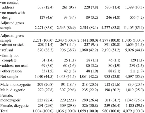
Table 1 shows distributions of the gross and net samples differentiated by cohort. 10.5 percent of the addresses in the gross sample were invalid contact addresses and 4.2 percent did not comply with the requirements of the design, leav-ing an adjusted gross sample of 11,405 cases. In cohorts 1 to 3, around 10 percent of the cases in the adjusted gross sample were permanently absent or sick during

Table 1 Gross and net samples of TwinLife

Cohort 1 (%) Cohort 2 (%) Cohort 3 (%) Cohort 4 (%) Total (%) Gross sample 2,736 (100.0) 2,697 (100.0) 2,823 (100.0) 5,103 (100.0) 13,359 (100.0)

঻no contact

address 338 (12.4) 261 (9.7) 220 (7.8) 580 (11.4) 1,399 (10.5) ঻no match with

design 127 (4.6) 93 (3.4) 89 (3.2) 246 (4.8) 555 (4.2) Adjusted gross

sample 2,271 (83.0) 2,343 (86.9) 2,514 (89.1) 4,277 (83.8) 11,405 (85.4) Adjusted gross

sample 2,271 (100.0) 2,343 (100.0) 2,514 (100.0) 4,277 (100.0) 11,405 (100.0) ঻absent or sick 258 (11.4) 267 (11.4) 237 (9.4) 891 (20.8) 1,653 (14.5) ঻refusal 870 (38.3) 906 (38.7) 1,060 (42.2) 2,190 (51.2) 5,026 (44.1) ঻family not

complete 31 (1.4) 25 (1.1) 28 (1.1) 45 (1.1) 129 (1.1) ঻address not used 69 (3.0) 60 (2.6) 80 (3.2) 80 (1.9) 289 (2.5) ঻other reason 33 (1.5) 42 (1.8) 48 (1.9) 88 (2.1) 211 (1.9) Net sample 1,010 (44.5) 1,043 (44.5) 1,061 (42.2) 983 (23.0) 4,097 (35.9) Male, monozygotic 209 (20.8) 191 (18.4) 218 (20.6) 212 (21.6) 830 (20.4) Male, dizygotic 279 (27.8) 307 (29.6) 235 (22.2) 198 (20.2) 1,019 (25.0) Female,

monozygotic 225 (22.4) 229 (22.1) 280 (26.4) 311 (31.7) 1,045 (25.6) Female, dizygotic 291 (29.0) 309 (29.8) 326 (30.8) 259 (26.4) 1,185 (29.1) Total 1,004 (100.0) 1,036 (100.0) 1,059 (100.0) 980 (100.0) 4,079 (100.0)

Note: The number of families used in this study declines to 4,079 compared to the net sample since in 11 families the multiples are triplets and for seven twin pairs no information about their zygosity is available.

(7)

the field phase and 40 percent refused to participate. In cohort 4, the sickness rate was twice as high and half of the sample refused participation. In 1.1 percent of the cases, it was not possible to interview all the necessary family members according to the design requirements, 2.5 percent of the addresses were not used because the target sample size had already been obtained, and 1.9 percent of the cases did not participate for other reasons.

This results in a net sample for wave 1 of 1,010 families in cohort 1, 1,043 families in cohort 2, 1,060 families in cohort 3, and 984 families in cohort 4, which closely matches the target sample size. The participation rate based on the adjusted gross sample is therefore over 40 percent in cohorts 1 to 3 and 23.0 percent in cohort 4. A total of 39 percent of the families in the net sample are part of the base sample, 51 percent are part of the urban sample, and 10.1 percent are part of the rural sample. For more information on the field process see Brix et al. (2017).

The lower part of Table 1 displays distributions by sex and zygosity of the twin pairs over the four cohorts for the net sample of the TwinLife panel.4_There

are more dizygotic than monozygotic twin pairs in cohorts 1 to 3, and in cohort 4 the share of monozygotic twin pairs is 53.3 percent. These results indicate that the probability-based sampling design used for TwinLife successfully counteracted the overrepresentation of monozygotic twins typically characterizing twin samples based on self-recruitment (i.e, two-thirds monozygotic twin pairs, with overrep-resentation particularly pronounced in adult samples, Lykken et al., 1987). The findings are also in line with research showing an increase in dizygotic twining rates for OECD countries, including Germany, since the 1980s (Hoekstra et al., 2008). This is primarily because dizygotic twinning is more strongly influenced by environmental factors such as the increase in maternal age at childbirth over recent decades (Lambalk et al., 1998). Overall, the distributions demonstrate that the TwinLife sample enables genetic sensitive analyses differentiated by gender and age.

As described above, both twins, one sibling, their parents, and the partners of the adult twins are the target respondents for the interviews, irrespective of whether they live in the same household or not. Table 2 shows the composition of the fami-lies (upper part of Table 2) and the households (lower part of Table 2) interviewed in TwinLife, wave 1. Overall, the TwinLife net sample consists of 4,097 twin families living in 4,828 households. A total of 91.4 percent of these families are families with two parents.5_{However, the share of two-parent families decreases over the}

4 In 50 of these families, second twin pairs exist; in 38 cases these are full siblings of the other twins, in eight cases, they are half-siblings, and in three cases, step-siblings. Moreover, one of the families has full sibling triplets in addition to the twins.

(8)

cohorts from 95.6 percent to 87.1 percent. In 62.2 percent of the families the twins have at least one sibling. Since parents of the earlier born twin cohorts had more time to have additional children, this share increases from 54.9 percent in cohort 1 to around 65 percent in cohorts 2 to 4. The mean number of siblings per family in families with at least one sibling is 1.6, and the maximum number of siblings is ten. Overall, the distributions indicate that TwinLife facilitates studies based on the ETFD.

The lower part of Table 2 illustrates the distribution of households in TwinLife across cohorts. As required by the study design, all of the twins in cohorts 1 and 2, and almost all of the twins in cohort 3 live together in one household. In more than 90 percent of the twin households in cohort 1, the twins live with two parents. This share drops to about 75 percent in cohort 3. For cohort 4, the share of twin

Table 2 Family and household compositions in the net sample of TwinLife

Cohort 1

(%) Cohort 2(%) Cohort 3(%) Cohort 4(%) Total(%)

Family composition

Mother and father, twins 431 (42.7) 337 (32.3) 350 (33.0) 290 (29.5) 1,408 (34.4) Mother and father, twins,

sibling 534 (52.9) 644 (61.7) 591 (55.7) 566 (57.6) 2,335 (57.0) Mother or father, twins 25 (2.5) 23 (2.2) 46 (4.3) 45 (4.6) 139 (3.4) Mother or father, twins, sibling 20 (2.0) 39 (3.7) 74 (7.0) 78 (7.9) 211 (5.2) No parents, (sibling)a _{0 (0)} _{0 (0)} _{0 (0)} _{4 (0.4)} _{4 (0.1)}

Total 1,010 (100) 1,043 (100) 1,061 (100) 983 (100) 4,097 (100)

Household composition

Parents, both twins, (sibling)b _{917 (90.3) 883 (83.4) 815 (74.1) 428 (25.9) 3,043 (63.0)}

Parent, both twins, (sibling)b _{93 (9.2) 160 (15.1) 231 (21.0) 113 (6.8) 597 (12.4)}

Parent(s), one twin, (sibling)b _{0 (0)} _{0 (0)} _{22 (2.0) 184 (11.1)} _{206 (4.3)}

Both twins, (sibling)b _{0 (0)} _{0 (0)} _{0 (0)} _{84 (5.1)} _{84 (1.7)}

One twin, (sibling)b _{0 (0)} _{0 (0)} _{8 (0.7) 532 (32.2) 540 (11.2)}

No twins 6 (0.6) 16 (1.5) 24 (2.2) 312 (18.9) 358 (7.4) Total 1,016 (100) 1,059 (100) 1,100 (100) 1,653 (100) 4,828 (100)

a_{Orphan families; three with at least one sibling and one with no sibling.} b_{Living in a household either with or without at least one sibling.}

(9)

households with at least one parent is 54.1 percent. This corresponds to 43.9 percent of all households in cohort 4. A total of 76 percent of the twins from cohort 4 who had already moved out of the parental household are living without their co-twin. This represents 32.2 percent of all households in cohort 4. Further, the share of non-twin households increases from approximately 1 percent in cohorts 1 to 3 to 18.9 percent in cohort 4. These results illustrate that TwinLife captures the major shift in household structures resulting from the young adult twins starting to create their own families.6

The TwinLife sample for our comparisons comprises all twin households in which at least one twin resides together with at least one parent of the twins. This household definition is close to the household definition of the Microcensus (see section The Microcensus Comparison Samples) and retains most of the TwinLife families in the sample. This parent-twin sample consists of 3,640 (out of 4,828) households in TwinLife. For cohorts 1 to 3 almost all twin families and households are included in this sample. Within cohort 4, the sample covers 73.8 percent of all families and 54.1 percent of all households with twins.

The Microcensus Comparison Samples

The comparison samples we use for this study are based on the German Micro-census 2013. The MicroMicro-census is a household survey based on a nationally repre-sentative sample of one percent (Destatis, 2014a, 2014b; Lengerer et al., 2007).7 While the sampling of TwinLife is focused on families defined by the ETFD, the sampling design of the Microcensus is based on households, specifically persons living together at the same address sampled from the population register (Lengerer et al. 2005).

As the Microcensus survey does not collect information on whether the chil-dren living in the household are twins or not, we need to construct a suitable com-parison sample to match the cohort and person composition of the TwinLife parent-twin sample described above without this information. Therefore, we define two different household samples – the multiple-child and the proxy-twin sample – based on the Microcensus. First, the multiple-childsample consists of one-family house-holds with one or two parents and at least two children under the age of 25 of which at least one child – the “anchor child” – belongs to the same birth cohorts as in TwinLife. Second, the proxy-twinsample contains one-family households in which

6 43.4 percent of the twins in cohort 4 have a partner and 30.7 percent of these twins live in a household with their partners.

(10)

two children of the same sex are born in the same year and live with at least one of their parents.

In view of the approximately 7,000 same-sex twin births each year (Destatis, 2013), we can expect to find around 70 proxy-twins in the 2013 Microcensus for each year of birth from circa 2000 and declining numbers for the years prior to 2000 based on the following assumptions: 1) a household sample of one percent from the population approximates a population sample of one percent; 2) there are only rare cases, other than twin births, of same-sex children in a household being born in the same year; 3) most twin children live together and with at least one parent.8_{To gain a proxy-twin sample of sufficient size for socio-demographic}

dif-ferentiated analyses, we use six-year birth cohorts: 2007-2012 (cohort 1), 2001-2006 (cohort 2), 1995-2000 (cohort 3), and 1989–1994 (cohort 4).

Moreover, to match the TwinLife sampling design, households in communities with fewer than 5,000 inhabitants are excluded. These represent about 16 percent of the households in the multiple-child and the proxy-twin Microcensus samples. This leaves us with 24,271 multiple-child and 1,039 proxy-twin households for our analysis.

Indicators

With respect to the social structural indicators used for the analysis, we compare household structures, the size of the communities where the household is located, German citizenship status on the household level, highest education of parents in the household, and also monthly net equivalent household income in euros. To assess the potential use of the TwinLife study for multidimensional analysis of social structural (dis-)advantage, we also compare the bivariate distributions of highest education in the household by monthly net equivalent household income. Moreover, we contrast maternal age at birth of the twins or the anchor child as a potential reason for social structural differences between the samples since giving birth later in life could be correlated with higher educational degrees or higher earnings.

The size of the community where the household is located is categorized based on the German community size classification (GKPOL). German citizenship is used as a proxy for migration background since the alternative indicators for migration background available in TwinLife and the Microcensus are not compa-rable. We assign German citizenship status on the household level if both parents

(11)

have German citizenship. The highest education within the household is based on the International Standard Classification of Education (ISCED) 1997 (Schneider, 2008). The individual-level information on parents’ education is used to calculate the highest obtained degree on the household level. The ISCED is coded as an ordered categorical variable with “no educational degree” (1) as the lowest and “Ph.D. degree” (6) as the highest category. Information on monthly net income is surveyed on the household level. To make the household incomes comparable across different household structures, an equivalence weight according to the new OECD scheme (OECD 2011) and an adjustment for inflation dividing the nominal income by the Consumer Price Index for Germany using 2015 as base year are applied.

Methods

To assess whether distributions of the social background indicators differ between the samples, we construct categorical variables based on these indicators and calculate the proportion of each category for the distributions of these categori-cal variables. In addition, we perform z-tests on equality of proportions between samples using the 95% confidence level and report their statistical significance for the substantial differences discussed in this paper. Cell-specific case numbers in the Microcensus proxy-twin sample are too small to show detailed distributions for highest ISCED in households and net equivalent monthly household income. Thus, we present ISCED levels 5a and 6 versus all lower levels and household’s median income. For maternal age at childbirth, we compare the means.

To account for missing values in education, citizenship and monthly net household income in the TwinLife sample, we set up a multiple imputation model on the household level.9_{We impute 20 values for each missing observation using}

multiple imputation with chained equations (van Buuren et al., 2006), a method which iterates over a sequence of univariate imputation models for each variable. For the univariate imputation models, we use predictive mean matching with ten nearest neighbors in case of continuous variables and logistic or ordered logistic regressions in case of categorical variables.10 The procedure assumes that the data is missing at random conditional on the predictors used. To preferably ensure that

9 Information is missing on ISCED for 4.5 percent of the mothers and 22.9 percent of the fathers, on German citizenship status for 4 percent of the mothers and 22.6 percent of the fathers, and on monthly net household income for 12.2 percent of the households. 10 The values presented in the descriptions are calculated as the mean of imputations in

(12)

this assumption is met, we use a comprehensive set of predictors.11_{We assess the}

influence of the imputation procedure on the distributions of the social structural indicators compared. Here, we find slight increases in the lower categories of the indicators (typically about 2 percent) and converse declines in the upper catego-ries. However, there are only minor differences between imputed and non-imputed estimates. Thus, in the following results section, we refrain from presenting non-imputed in addition to non-imputed results for reasons of clarity and brevity.

Results

Comparisons of the Social Background Indicators

In this section, we present the results of the comparisons of the distributions of the social background indicators in the TwinLife parent-child, the Microcensus proxy-twin, and the Microcensus multiple-child sample.

Household Structure

Table 3 shows the household structures in the TwinLife parent-twin sample in con-trast to the two Microcensus comparison samples. The number of children living in a household with both parents differs in the Microcensus multiple-child sample compared to the TwinLife parent-twin and the Microcensus proxy-twin samples.

While there are 58.9 percent of households with two children and both parents in the former sample, this share is approximately 40 percent in the latter two. This difference is plausible since potential parents often plan to have two children but if the second birth is a twin birth, they have three children (Ruckdeschel, 2007). The share of single-parent households is about 16 percent in all three samples. Overall, these results indicate that the main difference in the composition of twin and non-twin multiple-child households is the higher prevalence of households with two children in the latter group. In addition, the findings confirm that the probability-based sampling procedure used for TwinLife was appropriate in this regard since the household structures in the TwinLife parent-twin and the Microcensus proxy-twin samples are similar.

(13)

Table 3 Household structures in the TwinLife and Microcensus comparison samples

Cohort 1

(%) Cohort 2(%) Cohort 3(%) Cohort 4(%) Total(%)

TwinLife parent-twin sample

Couples, twin(s) 428 (42.4) 355 (34.0) 401 (38.3) 259 (47.9) 1443 (39.6) Couples, twin(s), sibling 489 (48.4) 528 (50.6) 414 (39.6) 169 (31.2) 1600 (44.0) Single parent, twin(s) 50 (5.0) 80 (7.7) 149 (14.2) 76 (14) 355 (9.8) Single parent, twin(s),

sibling 43 (4.3) 80 (7.7) 82 (7.8) 37 (6.8) 242 (6.6) Total 1,010 (100.0)1,043 (100.0)1,046 (100.0) 541 (100.0)3,640 (100.0)

Microcensus multiple-child sample

Couples, 2 children 3,680 (61.1) 3,523 (55.6) 3,531 (55.7) 3,558 (63.9)14,292 (58.9) Couples, 3 or more

children 1,713 (28.5) 1,774 (28.0) 1,544 (24.3) 948 (17.0) 5,979 (24.6) Single parent, 2

children 426 (7.1) 732 (11.5) 958 (15.1) 924 (16.6) 3,040 (12.5) Single parent, 3+

children 199 (3.3) 310 (4.9) 309 (4.9) 142 (2.5) 960 (4.0) Total 6,018 (100.0)6,339 (100.0)6,342 (100.0)5,572 (100.0) 24,271 (100)

Microcensus proxy-twin sample

Couples, 2 children 139 (46.8) 82 (28.3) 99 (33.2) 70 (45.5) 390 (37.5) Couples, 3 or more

children 122 (41.1) 149 (51.4) 139 (46.6) 48 (31.2) 458 (44.1) Single parent, 2

children 20 (6.7) 34 (11.7) 30 (10.1) 27 (17.5) 111 (10.7) Single parent, 3+

children 16 (5.4) 25 (8.6) 30 (10.1) 9 (5.8) 80 (7.7) Total 297 (100.0) 290 (100.0) 298 (100.0) 154 (100.0)1,039 (100.0)

Sources: TwinLife (doi: 10.4232/1.12665) and Microcensus 2013, own calculations

Community Size

Table 4 reports shares of households by community size across the three samples. Around two-thirds of the TwinLife households are located in communities with 50,000 or more inhabitants while this share is around 40 percent in the Microcen-sus samples.

(14)

Strategy). However, if we exclude the oversampled urban population, the distri-butions of the TwinLife and Microcensus samples are roughly comparable. The group of TwinLife households in communities with 500,000 or more inhabitants is around four percentage points larger than the Microcensus samples, and the share of households in communities with 100,000 to 499,999 inhabitants is approxi-mately six percentage points smaller in the TwinLife sample than in the Microcen-sus samples. The latter of these two differences is statistically significant. Regard-ing the Microcensus proxy-twin and multi-child samples, there are no considerable differences in shares of households by community size between the samples.

Table 4 Households by community size in percent

Cohort 1 Cohort 2 Cohort 3 Cohort 4 Total

5,000–19,999 (in %) 18.4 18.9 19.2 21.8 19.3

20,000–49,999 (in %) 10.5 13.3 10.9 14.1 12.0

50,000–99,999 (in %) 18.0 16.1 15.2 16.1 16.4

100,000–499,999 (in %) 21.9 21.1 22.6 20.5 21.7

> 500,000 (in %) 31.2 30.6 32.1 27.5 30.7

TwinLife, without urban sample

5,000–19,999 (in %) 38.4 37.4 39.0 37.0 38.1

20,000–49,999 (in %) 20.1 25.0 21.1 23.1 22.3

50,000–99,999 (in %) 10.1 9.3 8.8 10.5 9.5

100,000–499,999 (in %) 11.7 11.0 11.0 7.5 10.6

> 500,000 (in %) 19.7 17.3 20.1 22.0 19.5

5,000–19,999 (in %) 31.3 33.9 35.5 35.6 34.1

20,000–49,999 (in %) 22.1 23.8 23.5 24.1 23.4

50,000–99,999 (in %) 10.6 10.1 11.0 11.4 10.8

100,000–499,999 (in %) 17.4 16.2 15.9 15.6 16.3

> 500,000 (in %) 18.7 15.9 14.1 13.3 15.5

5,000–19,999 (in %) 26.6 33.8 35.6 31.8 32.0

20,000–49,999 (in %) 22.9 22.1 20.1 23.4 21.9

50,000–99,999 (in %) 11.5 11.0 12.1 13.6 11.8

100,000–499,999 (in %) 18.2 17.9 15.1 18.8 17.3

> 500,000 (in %) 20.9 15.2 17.1 12.3 16.9

(15)

Parental Citizenship Status

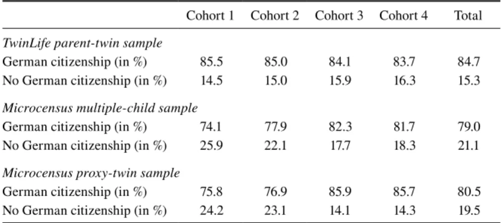
Table 5 contrasts the shares of households with German citizenship across the samples. Overall, this share is 84.7 percent in the TwinLife sample while the cor-responding shares are around 80 percent in the Microcensus samples. The share is constant across cohorts in the TwinLife sample while it declines in the Microcen-sus samples from about 85 percent in the older cohorts to about 75 percent in the younger cohorts. Consequently, there are around five to ten percentage points more households with German citizenship in the TwinLife sample for cohorts 1 and 2 and these differences are statistically significant. The shares of households with German citizenship in the Microcensus proxy-twin and multiple-child samples are similar.

Table 5 Households by German citizenship

German citizenship (in %) 85.5 85.0 84.1 83.7 84.7

No German citizenship (in %) 14.5 15.0 15.9 16.3 15.3

No German citizenship (in %) 25.9 22.1 17.7 18.3 21.1

No German citizenship (in %) 24.2 23.1 14.1 14.3 19.5 Sources: TwinLife (doi: 10.4232/1.12665) and Microcensus 2013, own calculations

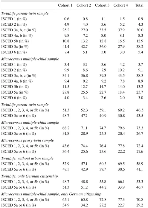
Parental Education

Table 6 describes the distributions of highest educational level in the households for the TwinLife parent-twin and the Microcensus multiple-child samples based on the ISCED.We observe that the TwinLife sample covers the full distribution of educational levels. The lower tail (ISCED 1 and 2) encompasses around 5 percent of the cases. The results indicate that there are more households with a university education (ISCED 5a and 6) and fewer with medium or low education (ISCED 1 to 3) in TwinLife than the Microcensus multiple-child sample, particularly in the younger cohorts.

(16)

house-Table 6 Highest educational level (based on ISCED) in household

ISCED 1 (in %) 0.6 0.8 1.1 1.5 0.9

ISCED 2 (in %) 4.9 4.0 3.6 5.2 4.3

ISCED 3a, b, c (in %) 25.2 27.0 33.5 37.9 30.0

ISCED 4a, b (in %) 9.8 7.2 8.0 8.1 8.3

ISCED 5b (in %) 10.8 13.2 12.8 16.5 12.9

ISCED 5a (in %) 41.4 42.7 36.0 27.9 38.2

ISCED 6 (in %) 7.4 5.1 5.0 3.0 5.4

ISCED 1 (in %) 3.4 3.7 3.6 4.2 3.7

ISCED 2 (in %) 9.9 8.6 7.9 10.2 9.1

ISCED 3a, b, c (in %) 34.1 36.8 39.3 43.5 38.3

ISCED 4a, b (in %) 9.4 9.2 9.2 7.8 8.9

ISCED 5b (in %) 11.5 12.7 14.7 14.0 13.2

ISCED 5a (in %) 27.8 25.5 22.7 18.4 23.7

ISCED 6 (in %) 4.0 3.4 2.6 2.0 3.0

ISCED 1, 2, 3, 4, or 5b (in %) 51.3 52.3 59.1 69.2 46.5

ISCED 5a or 6 (in %) 48.7 47.7 40.9 30.8 43.5

ISCED 1, 2, 3, 4, or 5b (in %) 68.2 71.1 74.7 79.6 73.3

ISCED 5a or 6 (in %) 31.8 28.9 25.3 20.4 26.7

ISCED 1, 2, 3, 4, or 5b (in %) 43.6 74.4 76.4 77.8 72.4

ISCED 5a or 6 (in %) 36.4 25.6 23.6 22.2 27.6

TwinLife, without urban sample

ISCED 1, 2, 3, 4, or 5b (in %) 52.9 57.1 60.3 69.5 58.9

ISCED 5a or 6 (in %) 47.1 42.9 39.7 30.5 41.1

TwinLife, only German citizenship

ISCED 1, 2, 3, 4, or 5b (in %) 48.7 48.8 55.8 66.1 53.3

ISCED 5a or 6 (in %) 51.3 51.2 44.2 33.9 46.7

Microcensus multiple-child sample, only German citizenship

ISCED 1, 2, 3, 4, or 5b (in %) 65.1 65.8 72.8 77.3 70.8

ISCED 5a or 6 (in %) 34.9 34.2 27.2 22.7 29.2

Note: Cell-specific case numbers in the Microcensus proxy-twin sample are too small to present detailed distributions for highest ISCED in households.

(17)

holds. Overall, the share of university educated households is 43.5 percent in the TwinLife sample while it is around 27 percent in the Microcensus samples. In cohort 4 the difference is around ten percentage points between the samples while it is between 15 and 20 percentage points in cohorts 1 to 3. All of these differences are statistically significant. The differences in younger cohorts decline slightly if we restrict the samples to households with German citizenship to account for the higher shares of these households in TwinLife.12_{The shares of households with a}

university education in the Microcensus proxy-twin and multiple-child samples are approximately the same.

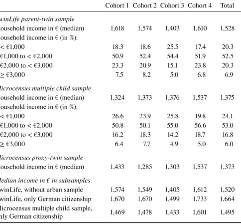
Household Income

Table 7 reports the distributions of monthly net equivalent household incomes for the TwinLife and Microcensus samples. It can be shown that the TwinLife sample covers the full income distribution. Across all cohorts, around 20 percent of the households have an adjusted income of less than €1,000 per month, around 53 per-cent have between €1,000 and €2,000 per month, around 20 perper-cent have between €2,000 and €3,000 per month, and approximately 7 percent have more than €3,000 per month.

These shares are roughly comparable to the Microcensus samples where the share of households with less than €1,000 per month is slightly higher and the share with between €2,000 and €3,000 per month is slightly lower. For these two income categories the differences between the TwinLife sample and the Microcensus sam-ples are statistically significant. Overall, the median monthly net equivalent house-hold income in the TwinLife sample is €1,528 while it is around €150 less in the Microcensus samples. Differentiated by cohort, these differences between monthly median incomes are approximately €100 in cohorts 3 and 4 and around €200 in cohorts 1 and 2. Restricting the TwinLife and Microcensus samples to households with German citizenship or excluding the TwinLife urban sample does not account for the differences observed. Conditional on parental education the household income medians are similar in the TwinLife and the Microcensus samples. This finding indicates that the differences in household income between the samples are mostly a consequence of the selective participation in TwinLife with respect to parental education (see sub-section Parental Education).

(18)

Table 7 Monthly net equivalent household income

Household income in € (median) 1,618 1,574 1,403 1,610 1,528 Household income in € (in %):

< €1,000 18.3 18.6 25.5 17.4 20.3

€1,000 to < €2,000 50.9 52.4 54.4 51.9 52.5

€2,000 to < €3,000 23.3 20.9 15.1 23.8 20.3

≥ €3,000 7.5 8.2 5.0 6.8 6.9

Microcensus multiple child sample

Household income in € (median) 1,324 1,373 1,376 1,537 1,375 Household income in € (in %):

< €1,000 26.6 23.9 25.8 19.8 24.1

€1,000 to < €2,000 50.8 50.1 55.0 56.6 53.0

€2,000 to < €3,000 16.2 18.3 14.2 18.7 16.8

≥ €3,000 6.4 7.7 4.9 5.0 6.0

Household income in € (median) 1,433 1,285 1,303 1,537 1,373

Median income in € in subsamples

TwinLife, without urban sample 1,574 1,549 1,405 1,612 1,520 TwinLife, only German citizenship 1,670 1,670 1,499 1,733 1,664 Microcensus multiple child sample,

only German citizenship 1,469 1,478 1,433 1,601 1,495

Note: Cell-specific case numbers in the Microcensus proxy-twin sample are too small to present detailed distributions for net equivalent monthly household income.

Sources: TwinLife (doi: 10.4232/1.12665) and Microcensus 2013, own calculations

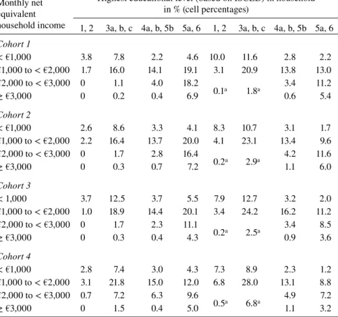
Parental Education and Household Income Combined

(19)

of between €1,000 and €2,000 and also those with low education (ISCED 1 or 2) and an income of less than €1,000 are lower.

Table 8 Highest educational level (ISCED) by net equivalent income in households

Monthly net equivalent household income

TwinLife parent-twin sample Microcensus multiple child sample Highest educational level (based on ISCED) in household

in % (cell percentages)

1, 2 3a, b, c 4a, b, 5b 5a, 6 1, 2 3a, b, c 4a, b, 5b 5a, 6

Cohort 1

< €1,000 3.8 7.8 2.2 4.6 10.0 11.6 2.8 2.2

€1,000 to < €2,000 1.7 16.0 14.1 19.1 3.1 20.9 13.8 13.0 €2,000 to < €3,000 0 1.1 4.0 18.2

0.1a _1.8a 3.4 11.2

≥ €3,000 0 0.2 0.4 6.9 0.6 5.4

Cohort 2

< €1,000 2.6 8.6 3.3 4.1 8.3 10.7 3.1 1.7

€1,000 to < €2,000 2.2 16.4 13.7 20.0 4.1 23.1 13.4 9.6 €2,000 to < €3,000 0 1.7 2.8 16.4

0.2a _2.9a 4.2 11.6

≥ €3,000 0 0.3 0.7 7.2 1.1 6.0

Cohort 3

< 1,000 3.7 12.5 3.7 5.5 7.9 12.7 3.2 2.0

€1,000 to < €2,000 1.0 18.9 14.4 20.1 3.4 24.2 16.2 11.2 €2,000 to < €3,000 0 1.7 2.3 11.1

0.2a _2.5a 3.4 8.5

≥ €3,000 0 0.3 0.4 4.3 0.9 3.6

Cohort 4

< €1,000 2.8 7.4 3.0 4.3 7.3 8.9 2.3 1.2

€1,000 to < €2,000 3.1 21.8 15.0 12.0 6.8 28.0 13.1 8.8 €2,000 to < €3,000 0.7 7.2 6.3 9.6

0.5a _6.8a 4.9 7.2

≥ €3,000 0 1.5 0.4 5.0 1.1 3.2

a_{Due to small sample sizes, the shares of the categories €2,000 to < €3,000 and ≥ €3,000}

are aggregated for ISCED 1, 2 and ISCED 3a, b, c.

(20)

Maternal Age at Birth

Finally, we compare the mean values of maternal age at the birth of the twins or the anchor child for the TwinLife and Microcensus samples. This value is approxi-mately 31 years in all samples and the differences between samples are statistically not significant. It increases from around 30 years in cohort 4 to about 32 years in cohort 1 which is accompanied by an increase in the share of mothers aged 35 or older at childbirth (from around 15 to 30 percent). The changes are less pronounced in the Microcensus multiple-child sample. Overall, there are no indications of dif-ferences in maternal age at childbirth which could be responsible for the social structural differences observed.

Limitations

With respect to the comparisons conducted in this study, the main limitation is the lack of a twin registry for Germany. Thus, we had to use a proxy-twin sample which is based on a one percent general population sample. As a result, the size of the proxy-twin sample is small. Moreover, we cannot conduct comparative analyses differentiating between monozygotic and dizygotic twins since there is no informa-tion on zygosity available for the proxy-twins. Nevertheless, our comparison sam-ples are based on the Microcensus, a survey of high quality standards, particularly regarding representativity (Lengerer et al., 2007). Therefore, the Microcensus is the best dataset available for conducting a study on the generalizability of socio-structural differentiated analyses of twins in Germany.

The central limitation our study found with respect to using TwinLife for such analyses is the slight selectivity of the TwinLife sample with respect to parental education and German citizenship. Partly, the underrepresentation of families without German citizenship is due to conducting the study only in German and restricting the sampling to families with sufficient proficiency of the German lan-guage (Brix et al., 2017). The underrepresentation of respondents with migration background – often corresponding with having no German citizenship – can com-monly be addressed using specialized sampling strategies (Brücker et al., 2014; Schupp & Wagner, 1995). However, TwinLife did not have funding for instruments in additional languages or an additional migration sample. A potential reason for the selectivity regarding parental education is the demanding questionnaire pro-gram for the first wave of TwinLife, particularly for the children aged around 5 at the time of the survey in cohort 1. To ensure panel stability, plans had already been made to shorten the survey for future TwinLife waves prior to the first wave and the program has been further reduced given the results of this study.13

(21)

Selectivity Correction

To address the selective participation in TwinLife with regard to parental education and German citizenship (see sub-sections Parental Citizenship Status and Paren-tal Education), we suggest conducting additional analyses using a cohort-specific weighting scheme based on the distribution of highest education in the households by German citizenship in the Microcensus multiple-child sample (see Appendix A). Since household income levels conditional on parental education are similar in both samples (see sub-section Household Income), we consider the differential incomes a consequence of the differences in education. In consequence, we did not include household income as additional indicator in our proposed weighting scheme. In principle, using such a weighting scheme for TwinLife is justified by the social structural similarity between (proxy-)twin and multiple-child households in Germany found in this study.

Conclusion

In this paper, we addressed two research questions regarding the generalizability of research on the gene-environment interplay utilizing the TwinLife data: first, we assessed the usability of the TwinLife sample for social stratified analyses of genetic influences; and second, we analyzed whether the social background of twin households in Germany is comparable to the whole population of multiple-child households. Furthermore, we introduced the design and sampling strategy of Twin-Life to assist researcher in using the TwinTwin-Life panel for their research.

Social Stratified Genetic Sensitive Analyses using TwinLife

Addressing our first research question, our comparison shows larger shares of urban households in TwinLife due to the oversampling of populous communities that was necessary to achieve the target sample size. Furthermore, the share of households with migration background – indicated by no German citizenship – is approximately five to ten percentage points smaller in the younger cohorts of the TwinLife compared to the Microcensus samples. Moreover, we show that the probability-based sampling of the TwinLife study was successful in counteracting the overrepresentation of monozygotic twins typical of twin samples based on self-recruitment (Lykken et al., 1987).

(22)

Twin-Life sample, particularly in the younger cohorts. The smaller share of households with no German citizenship in TwinLife can explain some of the differences in the shares of university educated households between the samples. For the monthly net equivalent household income, we found that median values were around €200 higher for the younger TwinLife cohorts and that the corresponding values were around €100 higher in the older cohorts. Additional analyses showed that the overs-ampling of urban communities in TwinLife cannot account for these differences.

In sum, our findings indicate that participation in TwinLife was, to some degree, selective with respect to parental education and German citizenship, spe-cifically in the younger cohorts. We proposed a weighting scheme to address this selectivity. However, since the TwinLife sample covers the whole distributions of the social background indicators, this selectivity does not restrict the usability of the TwinLife sample for social stratified analyses of genetic influences. In prin-ciple, TwinLife can be used for multidimensional analyses of genetic influences on social inequalities based on an ETFD.

Social Background Differences between Twin and

Multiple-child Households

Regarding our second research question, our analyses show that (proxy-)twin and multiple-child households in Germany have comparable distributions for many socio-demographic indicators such as community size, parental citizenship status, parental education, household income, and maternal age at birth of the twins or anchor children. The only difference we found between twin and multiple-child households is the higher prevalence of households with two children in the latter group. This difference can be explained by parents often planning to have two chil-dren (Ruckdeschel, 2007).

(23)

References

Brix, J., Pupeter, M., Rysina, A., Steinacker, G., Schneekloth, U., Baier, T., . . . Spinath, F. M. (2017). A longitudinal twin family study of the life course and individual develop-ment (TWINLIFE): Data collection and instrudevelop-ments of wave 1 face-to-face interviews. TwinLife Technical Report Series: Vol. 5. Bielefeld / Saarbrücken. Retrieved from https://pub.uni-bielefeld.de/record/2914569

Bronfenbrenner, U., & Ceci, S. J. (1994). Nature-nuture reconceptualized in developmental perspective: A bioecological model. Psychological Review, 101(4), p. 568–586. https://doi.org/10.1037/0033-295X.101.4.568

Brücker, H., Kroh, M., Bartsch, S., Goebel, J., Kühne, S., Liebau, E.,. . . Schupp, J. (2014).

The new IAB-SOEP migration sample: An introduction into the methodology and the contents. SOEP survey papers Series C, Data documentations: Vol. 216. Berlin: DIW. Retrieved from http://panel.gsoep.de/soep-docs/surveypapers/diw_ssp0216.pdf Destatis. (2013). Natürliche Bevölkerungsbewegung. Wiesbaden.

Destatis. (2014a). Bevölkerung und Erwerbstätigkeit – Haushalte und Familien: Ergebnisse des Mikrozensus 2013. Wiesbaden. https://doi.org/10.1007/978-3-658-11490-9_16 Destatis. (2014b). Mikrozensus 2013: Qualitätsbericht. Wiesbaden.

Diewald, M., Baier, T., Schulz, W., Schunck, R. (2016). Status attainment and social mobili-ty. How can genetics contribute to an understanding of their causes? In K. Hank & M. Kreyenfeld (eds), Social Demography Forschung an der Schnittstelle von Soziologie und Demografie. Kölner Zeitschrift für Soziologie und Sozialpsychologie (Sonderheft 55/2015, p. 371–395), Wiesbaden. https://doi.org/10.1007/978-3-658-11490-9_16 Falconer, D. S. (1960). Introduction to quantitative genetics. (1st_ed.)_{New York: Ronald}

Press Co.

Guo, G., & Stearns, E. (2000). The social influences on the realization of genetic potential for intellectual development, Social Forces, 80(3), p. 881–910.

https://doi.org/10.1353/sof.2002.0007

Hahn, E., Gottschling, J., Bleidorn, W., Kandler, C., Spengler, M., Kornadt, A. E., . . . Spinath, F. M. (2016). What drives the development of social inequality over the life course?: The German TwinLife Study. Twin Research and Human Genetics, 19(6), p. 659–672. https://doi.org/10.1017/thg.2016.76

Haworth, C. M. A., Wright, M. J., Luciano, M., Martin, N. G., de Geus, E. J. C., van Beijs-terveldt, C. E. M., . . . Plomin, R. (2010). The heritability of general cognitive ability increases linearly from childhood to young adulthood. Molecular Psychiatry, 15, p. 1112–1120. https://doi.org/10.1038/mp.2009.55

Hoekstra, C., Zhao, Z. Z., Lambalk, C. B., Willemsen, G., Martin, N. G., Boomsma, D. I., & Montgomery, G. W. (2008). Dizygotic twinning. Human Reproduction Update, 14(1), p. 37–47. https://doi.org/10.1093/humupd/dmm036

Lambalk, C. B., De Koning, C. H., & Braat, D. D. M. (1998). The endocrinology of di-zygotic twinning in the human, Molecular and Cellular Endocrinology, 145(1-2), p. 97–102. https://doi.org/10.1016/S0303-7207(98)00175-0

Lengerer, A., Bohr, J., & Janßen, A. (2005). Households, families and ways of life in the microcensus: concepts and stylizations (ZUMA-Arbeitsbericht). Mannheim.

Lengerer, A., Janßen, A., & Bohr, J. (2007). Possibilities for family research with the Ger-man Microcensus. Journal of Family Research, 19(2), p. 186–209.

(24)

Ligthart, L., Van Beijsterveldt, C., Kevenaar, S., De Zeeuw, E., Van Bergen, E., Bruins, S., . . . Boomsma, D. (2019). The Netherlands Twin Register: Longitudinal research based on twin and twin-family designs. Twin Research and Human Genetics, online first, p. 1–14. https://doi.org/10.1017/thg.2019.93

Lykken, D. T., McGue, M., & Tellegen, A. (1987). Recruitment bias in twin research: The rule of two-thirds reconsidered. Behavior Genetics, 17(4), p. 343–362.

http://dx.doi.org/10.1007/BF01068136

Mönkediek, B., Lang, V., Weigel, L., Baum, M., Eifler, E., Hahn, E., . . . Spinath, F. (2019). The German Twin Family Panel (TwinLife). Twin Research and Human Genetics, on-line first, p. 1–8. https://doi.org/10.1017/thg.2019.63

Nielsen, F. (2016). The status-achievement process: Insights from genetics. Frontiers in So-ciology,1(9), p. 1–15. https://doi.org/10.3389/fsoc.2016.00009

OECD. (2011). What Are Equivalence Scales?: OECD Project on Income Distribution and Poverty. Retrieved from

http://www.oecd.org/eco/growth/OECD-Note-EquivalenceScales.pdf, 25 April 2017 Plomin, R., DeFries, J. C., Knopik, V. S., & Neiderhiser, J. (2016). Behavioral genetics. (7th

ed.) New York: Worth Publishers.

Polderman, T. J. C., Benyamin, B., de Leeuw, C. A., Sullivan, P. F., van Bochoven, A., Vis-scher, P. M., & Posthuma, D. (2015). Meta-analysis of the heritability of human traits based on fifty years of twin studies. Nature Genetics 47(7), p. 702–709.

https://doi.org/10.1038/ng.3285

Ruckdeschel, K. (2007). Fertility intentions of childless persons. Journal of Family Re-search, 19(2), p. 210–230. https://nbn-resolving.org/urn:nbn:de:0168-ssoar-58113 Schneider, S. L. (2008). Applying the ISCED‐97 to the German educational qualifications.

In S. L. Schneider (Ed.), The International Standard Classification of Education (IS-CED-97). An evaluation of content and criterion validity for 15 European countries

(p. 76–102). Mannheim.

Schupp, J., & Wagner, G. G. (1995). Die Zuwanderer-Stichprobe des Sozio-ökonomischen Panels (SOEP). Vierteljahrshefte zur Wirtschaftsforschung, 64(1), p. 16–25.

https://www.econstor.eu/bitstream/10419/141079/1/vjh_v64_i01_pp016-025.pdf Selita, F., & Kovas, Y. (2019). Genes and Gini: What inequality means for heritability.

Jour-nal of Biosocial Science, 51(1), p. 18–47. https://doi.org/10.1017/S0021932017000645 Shanahan, M. J., & Hofer, S. M. (2005). Social context in gene-environment interactions:

Retrospect and prospect, The Journals of Gerontology: Series B, 60(1), p. 65–76. https://doi.org/10.1093/geronb/60.Special_Issue_1.65

Strenberg, A. (2013). Interpreting estimates of heritability – A note on the twin decomposi-tion, Economics and Human Biology, 11(2), p. 201–205.

https://doi.org/10.1016/j.ehb.2012.05.002

Tucker-Drob, E. M., & Bates, T.C. (2016) Large cross-national differences in gene × so-cioeconomic status interaction on intelligence. Psychological Science 27(2), p. 138– 149. https://doi.org/10.1177/0956797615612727

Turkheimer, E. (2000). Three laws of behavior genetics and what they mean. Current Direc-tions in Psychological Science, 9(5), p. 160–164.

https://doi.org/10.1111/1467-8721.00084

van Buuren, S., Brand, J. P. L., Groothuis-Oudshoorn, C. G. M., & Rubin, D. B. (2006). Fully conditional specification in multivariate imputation. Journal of Statistical Com-putation and Simulation, 76(12), p. 1049–1064.

(25)

Zagai, U., Lichtenstein, P., Pedersen, N., & Magnusson, P. (2019). The Swedish Twin Regis-try: Content and management as a research infrastructure. Twin Research and Human Genetics, online first, p. 1–9. https://doi.org/10.1017/thg.2019.99

(26)

Appendix A

Selectivity correction weighting scheme based on the Microcensus

This appendix contains instructions for constructing a weighting scheme matching the cohort specific highest ISCED by German citizenship distribution of parents on the household level for TwinLife analysis samples with the Microcensus multiple-child sample. The aim of the proposed weighting scheme is to address the selectiv-ity of the TwinLife sample regarding parental education and German citizenship status, particularly in the younger cohorts. We advise using it as a robustness check, i.e., to assess discrepancies in the results between analyses conducted with and without the weighting scheme. Comparable results in both analyses indicate that the conclusions drawn are not influenced by the selectivity.

We construct weights specific to each of the four TwinLife cohorts. First, for a cohort-specific weighting scheme like this, we need to calculate the shares of observations in the TwinLife analysis sample used by highest ISCED and German citizenship of the parents on the household level for each cohort using the categori-zation presented in Table A1. This share is given by the number of observations in a specific highest ISCED by German citizenship cell (J) for a specific cohort divided by the total number of observations in the analysis sample (N) for a specific cohort. Second, we need to divide the cell-specific correction factors (C) presented in Table A1 by the cohort-specific shares calculated for the analysis sample. The correc-tion factors in Table A1 are based on the cohort-specific shares of observacorrec-tions in the Microcensus multiple-child sample by highest ISCED and German citizenship. Hence, the cohort-specific weights (W) assigned to each observation in the analysis sample depending on highest parental ISCED and parental German citizenship on the household level are given conducting the following calculation:

W = C/(J/N) = C x N/J

(27)

Table A1 Factors for a selectivity correction weighting scheme based on Microcensus

Highest educational level (using ISCED) in household 1, 2 3a, 3b, 3c 4a, 4b, 5b 5a, 6

Cohort 1

German citizenship 0.05735661 0.24804655 0.17722361 0.25835412 No German citizenship 0.07547797 0.09293433 0.03142145 0.05918537

Cohort 2

Cohort 3

Cohort 4

Note: The correction factors in the table are not the weights. Please read Appendix A for instructions on how to construct weights using these correction factors.

(28)