A Taxonomy and Evaluation of Dense Two-Frame
Stereo Correspondence Algorithms
Daniel Scharstein
Richard Szeliski
Dept. of Math and Computer Science
Microsoft Research
Middlebury College
Microsoft Corporation
Middlebury, VT 05753
Redmond, WA 98052
[email protected]
[email protected]
Abstract
Stereo matching is one of the most active research areas in computer vision. While a large number of algorithms for stereo correspondence have been developed, relatively lit-tle work has been done on characterizing their performance. In this paper, we present a taxonomy of dense, two-frame stereo methods. Our taxonomy is designed to assess the dif-ferent components and design decisions made in individual stereo algorithms. Using this taxonomy, we compare exist-ing stereo methods and present experiments evaluatexist-ing the performance of many different variants. In order to estab-lish a common software platform and a collection of data sets for easy evaluation, we have designed a stand-alone, flexible C++ implementation that enables the evaluation of individual components and that can easily be extended to in-clude new algorithms. We have also produced several new multi-frame stereo data sets with ground truth and are mak-ing both the code and data sets available on the Web. Finally, we include a comparative evaluation of a large set of today’s best-performing stereo algorithms.
1. Introduction
Stereo correspondence has traditionally been, and continues to be, one of the most heavily investigated topics in computer vision. However, it is sometimes hard to gauge progress in the field, as most researchers only report qualitative results on the performance of their algorithms. Furthermore, a sur-vey of stereo methods is long overdue, with the last exhaus-tive surveys dating back about a decade [7, 37, 25]. This paper provides an update on the state of the art in the field, with particular emphasis on stereo methods that (1) operate on two frames under known camera geometry, and (2) pro-duce a dense disparity map, i.e., a disparity estimate at each pixel.
Our goals are two-fold:
1. To provide a taxonomy of existing stereo algorithms
that allows the dissection and comparison of individual algorithm components design decisions;
2. To provide a test bed for the quantitative evaluation of stereo algorithms. Towards this end, we are plac-ing sample implementations of correspondence algo-rithms along with test data and results on the Web at
www.middlebury.edu/stereo.
We emphasize calibrated two-frame methods in order to fo-cus our analysis on the essential components of stereo cor-respondence. However, it would be relatively straightfor-ward to generalize our approach to include many multi-frame methods, in particular multiple-baseline stereo [85] and its plane-sweep generalizations [30, 113].
The requirement of dense output is motivated by modern applications of stereo such as view synthesis and image-based rendering, which require disparity estimates in all im-age regions, even those that are occluded or without texture. Thus, sparse and feature-based stereo methods are outside the scope of this paper, unless they are followed by a surface-fitting step, e.g., using triangulation, splines, or seed-and-grow methods.
We begin this paper with a review of the goals and scope of this study, which include the need for a coherent taxonomy and a well thought-out evaluation methodology. We also review disparity space representations, which play a central role in this paper. In Section 3, we present our taxonomy of dense two-frame correspondence algorithms. Section 4 discusses our current test bed implementation in terms of the major algorithm components, their interactions, and the parameters controlling their behavior. Section 5 describes our evaluation methodology, including the methods we used for acquiring calibrated data sets with known ground truth. In Section 6 we present experiments evaluating the different algorithm components, while Section 7 provides an overall comparison of 20 current stereo algorithms. We conclude in Section 8 with a discussion of planned future work.
2. Motivation and scope
Compiling a complete survey of existing stereo methods, even restricted to dense two-frame methods, would be a formidable task, as a large number of new methods are pub-lished every year. It is also arguable whether such a survey would be of much value to other stereo researchers, besides being an obvious catch-all reference. Simply enumerating different approaches is unlikely to yield new insights.
Clearly, a comparative evaluation is necessary to assess the performance of both established and new algorithms and to gauge the progress of the field. The publication of a simi-lar study by Barron et al. [8] has had a dramatic effect on the development of optical flow algorithms. Not only is the per-formance of commonly used algorithms better understood by researchers, but novel publications have to improve in some way on the performance of previously published tech-niques [86]. A more recent study by Mitiche and Bouthemy [78] reviews a large number of methods for image flow com-putation and isolates central problems, but does not provide any experimental results.
In stereo correspondence, two previous comparative pa-pers have focused on the performance of sparse feature matchers [54, 19]. Two recent papers [111, 80] have devel-oped new criteria for evaluating the performance of dense stereo matchers for image-based rendering and tele-presence applications. Our work is a continuation of the investiga-tions begun by Szeliski and Zabih [116], which compared the performance of several popular algorithms, but did not provide a detailed taxonomy or as complete a coverage of algorithms. A preliminary version of this paper appeared in the CVPR 2001 Workshop on Stereo and Multi-Baseline Vision [99].
An evaluation of competing algorithms has limited value if each method is treated as a “black box” and only final results are compared. More insights can be gained by exam-ining the individual components of various algorithms. For example, suppose a method based on global energy mini-mization outperforms other methods. Is the reason a better energy function, or a better minimization technique? Could the technique be improved by substituting different matching costs?
In this paper we attempt to answer such questions by providing a taxonomy of stereo algorithms. The taxonomy is designed to identify the individual components and de-sign decisions that go into a published algorithm. We hope that the taxonomy will also serve to structure the field and to guide researchers in the development of new and better algorithms.
2.1. Computational theory
Any vision algorithm, explicitly or implicitly, makes as-sumptions about the physical world and the image formation process. In other words, it has an underlying computational
theory [74, 72]. For example, how does the algorithm mea-sure the evidence that points in the two images match, i.e., that they are projections of the same scene point? One com-mon assumption is that of Lambertian surfaces, i.e., surfaces whose appearance does not vary with viewpoint. Some al-gorithms also model specific kinds of camera noise, or dif-ferences in gain or bias.
Equally important are assumptions about the world or scene geometry and the visual appearance of objects. Starting from the fact that the physical world consists of piecewise-smooth surfaces, algorithms have built-in smoothness assumptions (often implicit) without which the correspondence problem would be underconstrained and ill-posed. Our taxonomy of stereo algorithms, presented in Sec-tion 3, examines both matching assumpSec-tions and smoothness assumptions in order to categorize existing stereo methods. Finally, most algorithms make assumptions about camera calibration and epipolar geometry. This is arguably the best-understood part of stereo vision; we therefore assume in this paper that we are given a pair of rectified images as input. Recent references on stereo camera calibration and rectification include [130, 70, 131, 52, 39].
2.2. Representation
A critical issue in understanding an algorithm is the represen-tation used internally and output externally by the algorithm. Most stereo correspondence methods compute a univalued disparity functiond(x, y)with respect to a reference image, which could be one of the input images, or a “cyclopian” view in between some of the images.
Other approaches, in particular multi-view stereo meth-ods, use multi-valued [113], voxel-based [101, 67, 34, 33, 24], or layer-based [125, 5] representations. Still other ap-proaches use full 3D models such as deformable models [120, 121], triangulated meshes [43], or level-set methods [38].
Since our goal is to compare a large number of methods within one common framework, we have chosen to focus on techniques that produce a univalued disparity mapd(x, y) as their output. Central to such methods is the concept of a disparity space(x, y, d). The term disparity was first intro-duced in the human vision literature to describe the differ-ence in location of corresponding features seen by the left and right eyes [72]. (Horizontal disparity is the most com-monly studied phenomenon, but vertical disparity is possible if the eyes are verged.)
In computer vision, disparity is often treated as synony-mous with inverse depth [20, 85]. More recently, several re-searchers have defined disparity as a three-dimensional pro-jective transformation (collineation or homography) of 3-D space(X, Y, Z). The enumeration of all possible matches in such a generalized disparity space can be easily achieved with a plane sweep algorithm [30, 113], which for every disparitydprojects all images onto a common plane using
a perspective projection (homography). (Note that this is different from the meaning of plane sweep in computational geometry.)
In general, we favor the more generalized interpretation of disparity, since it allows the adaptation of the search space to the geometry of the input cameras [113, 94]; we plan to use it in future extensions of this work to multiple images. (Note that plane sweeps can also be generalized to other sweep surfaces such as cylinders [106].)
In this study, however, since all our images are taken on a linear path with the optical axis perpendicular to the camera displacement, the classical inverse-depth interpretation will suffice [85]. The(x, y)coordinates of the disparity space are taken to be coincident with the pixel coordinates of a reference image chosen from our input data set. The corre-spondence between a pixel(x, y)in reference imagerand a pixel(x, y)in matching imagemis then given by
x=x+s d(x, y), y =y, (1)
wheres=±1is a sign chosen so that disparities are always positive. Note that since our images are numbered from leftmost to rightmost, the pixels move from right to left.
Once the disparity space has been specified, we can intro-duce the concept of a disparity space image or DSI [127, 18]. In general, a DSI is any image or function defined over a con-tinuous or discretized version of disparity space(x, y, d). In practice, the DSI usually represents the confidence or log likelihood (i.e., cost) of a particular match implied by
d(x, y).
The goal of a stereo correspondence algorithm is then to produce a univalued function in disparity spaced(x, y)that best describes the shape of the surfaces in the scene. This can be viewed as finding a surface embedded in the dispar-ity space image that has some optimaldispar-ity property, such as lowest cost and best (piecewise) smoothness [127]. Figure 1 shows examples of slices through a typical DSI. More figures of this kind can be found in [18].
3. A taxonomy of stereo algorithms
In order to support an informed comparison of stereo match-ing algorithms, we develop in this section a taxonomy and categorization scheme for such algorithms. We present a set of algorithmic “building blocks” from which a large set of existing algorithms can easily be constructed. Our taxonomy is based on the observation that stereo algorithms generally perform (subsets of) the following four steps [97, 96]:1. matching cost computation; 2. cost (support) aggregation;
3. disparity computation / optimization; and 4. disparity refinement.
The actual sequence of steps taken depends on the specific algorithm.
For example, local (window-based) algorithms, where the disparity computation at a given point depends only on intensity values within a finite window, usually make implicit smoothness assumptions by aggregating support. Some of these algorithms can cleanly be broken down into steps 1, 2, 3. For example, the traditional sum-of-squared-differences (SSD) algorithm can be described as:
1. the matching cost is the squared difference of intensity values at a given disparity;
2. aggregation is done by summing matching cost over square windows with constant disparity;
3. disparities are computed by selecting the minimal (win-ning) aggregated value at each pixel.
Some local algorithms, however, combine steps 1 and 2 and use a matching cost that is based on a support region, e.g. normalized cross-correlation [51, 19] and the rank transform [129]. (This can also be viewed as a preprocessing step; see Section 3.1.)
On the other hand, global algorithms make explicit smoothness assumptions and then solve an optimization problem. Such algorithms typically do not perform an ag-gregation step, but rather seek a disparity assignment (step 3) that minimizes a global cost function that combines data (step 1) and smoothness terms. The main distinction be-tween these algorithms is the minimization procedure used, e.g., simulated annealing [75, 6], probabilistic (mean-field) diffusion [97], or graph cuts [23].
In between these two broad classes are certain iterative algorithms that do not explicitly state a global function that is to be minimized, but whose behavior mimics closely that of iterative optimization algorithms [73, 97, 132]. Hierar-chical (coarse-to-fine) algorithms resemble such iterative al-gorithms, but typically operate on an image pyramid, where results from coarser levels are used to constrain a more local search at finer levels [126, 90, 11].
3.1. Matching cost computation
The most common pixel-based matching costs include squared intensity differences (SD) [51, 1, 77, 107] and abso-lute intensity differences (AD) [58]. In the video processing community, these matching criteria are referred to as the mean-squared error (MSE) and mean absolute difference (MAD) measures; the term displaced frame difference is also often used [118].
More recently, robust measures, including truncated quadratics and contaminated Gaussians have been proposed [15, 16, 97]. These measures are useful because they limit the influence of mismatches during aggregation.
(a) (b) (c) (d) (e)
(f)
Figure 1: Slices through a typical disparity space image (DSI): (a) original color image; (b) ground-truth disparities; (c–e) three(x, y)
slices ford= 10,16,21; (e) an(x, d)slice fory= 151(the dashed line in Figure (b)). Different dark (matching) regions are visible in Figures (c–e), e.g., the bookshelves, table and cans, and head statue, while three different disparity levels can be seen as horizontal lines in the(x, d)slice (Figure (f)). Note the dark bands in the various DSIs, which indicate regions that match at this disparity. (Smaller dark regions are often the result of textureless regions.)
Other traditional matching costs include normalized cross-correlation [51, 93, 19], which behaves similar to sum-of-squared-differences (SSD), and binary matching costs (i.e., match / no match) [73], based on binary features such as edges [4, 50, 27] or the sign of the Laplacian [82]. Bi-nary matching costs are not commonly used in dense stereo methods, however.
Some costs are insensitive to differences in camera gain or bias, for example gradient-based measures [100, 95] and non-parametric measures such as rank and census transforms [129]. Of course, it is also possible to correct for differ-ent camera characteristics by performing a preprocessing step for bias-gain or histogram equalization [48, 32]. Other matching criteria include phase and filter-bank responses [74, 63, 56, 57]. Finally, Birchfield and Tomasi have pro-posed a matching cost that is insensitive to image sampling [12]. Rather than just comparing pixel values shifted by inte-gral amounts (which may miss a valid match), they compare each pixel in the reference image against a linearly interpo-lated function of the other image.
The matching cost values over all pixels and all disparities form the initial disparity space imageC0(x, y, d). While our study is currently restricted to two-frame methods, the ini-tial DSI can easily incorporate information from more than two images by simply summing up the cost values for each matching imagem, since the DSI is associated with a fixed reference imager(Equation (1)). This is the idea behind multiple-baseline SSSD and SSAD methods [85, 62, 81]. As mentioned in Section 2.2, this idea can be generalized to arbitrary camera configurations using a plane sweep algo-rithm [30, 113].
3.2. Aggregation of cost
Local and window-based methods aggregate the matching cost by summing or averaging over a support region in
the DSI C(x, y, d). A support region can be either two-dimensional at a fixed disparity (favoring fronto-parallel surfaces), or three-dimensional inx-y-dspace (supporting slanted surfaces). Two-dimensional evidence aggregation has been implemented using square windows or Gaussian convolution (traditional), multiple windows anchored at dif-ferent points, i.e., shiftable windows [2, 18], windows with adaptive sizes [84, 60, 124, 61], and windows based on connected components of constant disparity [22]. Three-dimensional support functions that have been proposed in-clude limited disparity difference [50], limited disparity gra-dient [88], and Prazdny’s coherence principle [89].
Aggregation with a fixed support region can be performed using 2D or 3D convolution,
C(x, y, d) =w(x, y, d)∗C0(x, y, d), (2)
or, in the case of rectangular windows, using efficient (mov-ing average) box-filters. Shiftable windows can also be implemented efficiently using a separable sliding min-filter (Section 4.2). A different method of aggregation is itera-tive diffusion, i.e., an aggregation (or averaging) operation that is implemented by repeatedly adding to each pixel’s cost the weighted values of its neighboring pixels’ costs [114, 103, 97].
3.3. Disparity computation and optimization
Local methods. In local methods, the emphasis is on the
matching cost computation and on the cost aggregation steps. Computing the final disparities is trivial: simply choose at each pixel the disparity associated with the minimum cost value. Thus, these methods perform a local “winner-take-all” (WTA) optimization at each pixel. A limitation of this approach (and many other correspondence algorithms) is that uniqueness of matches is only enforced for one image (the reference image), while points in the other image might
get matched to multiple points.
Global optimization. In contrast, global methods perform
almost all of their work during the disparity computation phase and often skip the aggregation step. Many global methods are formulated in an energy-minimization frame-work [119]. The objective is to find a disparity functiond that minimizes a global energy,
E(d) =Edata(d) +λEsmooth(d). (3) The data term,Edata(d), measures how well the disparity functiondagrees with the input image pair. Using the dis-parity space formulation,
Edata(d) =
(x,y)
C(x, y, d(x, y)), (4)
whereCis the (initial or aggregated) matching cost DSI. The smoothness termEsmooth(d)encodes the smooth-ness assumptions made by the algorithm. To make the opti-mization computationally tractable, the smoothness term is often restricted to only measuring the differences between neighboring pixels’ disparities,
Esmooth(d) =
(x,y)
ρ(d(x, y)−d(x+1, y)) +
ρ(d(x, y)−d(x, y+1)), (5)
whereρis some monotonically increasing function of dis-parity difference. (An alternative to smoothness functionals is to use a lower-dimensional representation such as splines [112].)
In regularization-based vision [87],ρis a quadratic func-tion, which makesdsmooth everywhere and may lead to poor results at object boundaries. Energy functions that do not have this problem are called discontinuity-preserving and are based on robustρfunctions [119, 16, 97]. Geman and Geman’s seminal paper [47] gave a Bayesian interpreta-tion of these kinds of energy funcinterpreta-tions [110] and proposed a discontinuity-preserving energy function based on Markov Random Fields (MRFs) and additional line processes. Black and Rangarajan [16] show how line processes can be often be subsumed by a robust regularization framework.
The terms inEsmooth can also be made to depend on the intensity differences, e.g.,
ρd(d(x, y)−d(x+1, y))·ρI(I(x, y)−I(x+1, y)), (6)
whereρI is some monotonically decreasing function of tensity differences that lowers smoothness costs at high in-tensity gradients. This idea [44, 42, 18, 23] encourages dis-parity discontinuities to coincide with intensity/color edges and appears to account for some of the good performance of global optimization approaches.
Once the global energy has been defined, a variety of al-gorithms can be used to find a (local) minimum. Traditional approaches associated with regularization and Markov Ran-dom Fields include continuation [17], simulated annealing [47, 75, 6], highest confidence first [28], and mefield an-nealing [45].
More recently, max-flow and graph-cut methods have been proposed to solve a special class of global optimiza-tion problems [92, 55, 23, 123, 65]. Such methods are more efficient than simulated annealing and have produced good results.
Dynamic programming. A different class of global
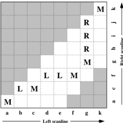
opti-mization algorithms are those based on dynamic program-ming. While the 2D-optimization of Equation (3) can be shown to be NP-hard for common classes of smoothness functions [123], dynamic programming can find the global minimum for independent scanlines in polynomial time. Dy-namic programming was first used for stereo vision in sparse, edge-based methods [3, 83]. More recent approaches have focused on the dense (intensity-based) scanline optimization problem [10, 9, 46, 31, 18, 13]. These approaches work by computing the minimum-cost path through the matrix of all pairwise matching costs between two corresponding scan-lines. Partial occlusion is handled explicitly by assigning a group of pixels in one image to a single pixel in the other image. Figure 2 shows one such example.
Problems with dynamic programming stereo include the selection of the right cost for occluded pixels and the difficulty of enforcing inter-scanline consistency, al-though several methods propose ways of addressing the lat-ter [83, 9, 31, 18, 13]. Another problem is that the dynamic programming approach requires enforcing the monotonicity or ordering constraint [128]. This constraint requires that the relative ordering of pixels on a scanline remain the same between the two views, which may not be the case in scenes containing narrow foreground objects.
Cooperative algorithms. Finally, cooperative
algo-rithms, inspired by computational models of human stereo vision, were among the earliest methods proposed for dis-parity computation [36, 73, 76, 114]. Such algorithms it-eratively perform local computations, but use nonlinear op-erations that result in an overall behavior similar to global optimization algorithms. In fact, for some of these algo-rithms, it is possible to explicitly state a global function that is being minimized [97]. Recently, a promising variant of Marr and Poggio’s original cooperative algorithm has been developed [132].
3.4. Refinement of disparities
Most stereo correspondence algorithms compute a set of disparity estimates in some discretized space, e.g., for
inte-c d e f g k a
Left scanline
i
Right scanline
ac
f
g
jk
h
b
M L
R R R
M
L L M
M M
Figure 2: Stereo matching using dynamic programming. For each
pair of corresponding scanlines, a minimizing path through the matrix of all pairwise matching costs is selected. Lowercase letters (a–k) symbolize the intensities along each scanline. Uppercase letters represent the selected path through the matrix. Matches are indicated by M, while partially occluded points (which have a fixed cost) are indicated by L and R, corresponding to points only visible in the left and right image, respectively. Usually, only a limited disparity range is considered, which is 0–4 in the figure (indicated by the non-shaded squares). Note that this diagram shows an “unskewed”x-dslice through the DSI.
ger disparities (exceptions include continuous optimization techniques such as optic flow [11] or splines [112]). For ap-plications such as robot navigation or people tracking, these may be perfectly adequate. However for image-based ren-dering, such quantized maps lead to very unappealing view synthesis results (the scene appears to be made up of many thin shearing layers). To remedy this situation, many al-gorithms apply a sub-pixel refinement stage after the initial discrete correspondence stage. (An alternative is to simply start with more discrete disparity levels.)
Sub-pixel disparity estimates can be computed in a va-riety of ways, including iterative gradient descent and fit-ting a curve to the matching costs at discrete disparity lev-els [93, 71, 122, 77, 60]. This provides an easy way to increase the resolution of a stereo algorithm with little addi-tional computation. However, to work well, the intensities being matched must vary smoothly, and the regions over which these estimates are computed must be on the same (correct) surface.
Recently, some questions have been raised about the ad-visability of fitting correlation curves to integer-sampled matching costs [105]. This situation may even be worse when sampling-insensitive dissimilarity measures are used [12]. We investigate this issue in Section 6.4 below.
Besides sub-pixel computations, there are of course other ways of post-processing the computed disparities. Occluded areas can be detected using cross-checking (comparing left-to-right and right-to-left disparity maps) [29, 42]. A median
filter can be applied to “clean up” spurious mismatches, and holes due to occlusion can be filled by surface fitting or by distributing neighboring disparity estimates [13, 96]. In our implementation we are not performing such clean-up steps since we want to measure the performance of the raw algorithm components.
3.5. Other methods
Not all dense two-frame stereo correspondence algorithms can be described in terms of our basic taxonomy and rep-resentations. Here we briefly mention some additional al-gorithms and representations that are not covered by our framework.
The algorithms described in this paper first enumerate all possible matches at all possible disparities, then select the best set of matches in some way. This is a useful approach when a large amount of ambiguity may exist in the com-puted disparities. An alternative approach is to use meth-ods inspired by classic (infinitesimal) optic flow computa-tion. Here, images are successively warped and motion esti-mates incrementally updated until a satisfactory registration is achieved. These techniques are most often implemented within a coarse-to-fine hierarchical refinement framework [90, 11, 8, 112].
A univalued representation of the disparity map is also not essential. Multi-valued representations, which can rep-resent several depth values along each line of sight, have been extensively studied recently, especially for large multi-view data set. Many of these techniques use a voxel-based representation to encode the reconstructed colors and spatial occupancies or opacities [113, 101, 67, 34, 33, 24]. Another way to represent a scene with more complexity is to use mul-tiple layers, each of which can be represented by a plane plus residual parallax [5, 14, 117]. Finally, deformable surfaces of various kinds have also been used to perform 3D shape reconstruction from multiple images [120, 121, 43, 38].
3.6. Summary of methods
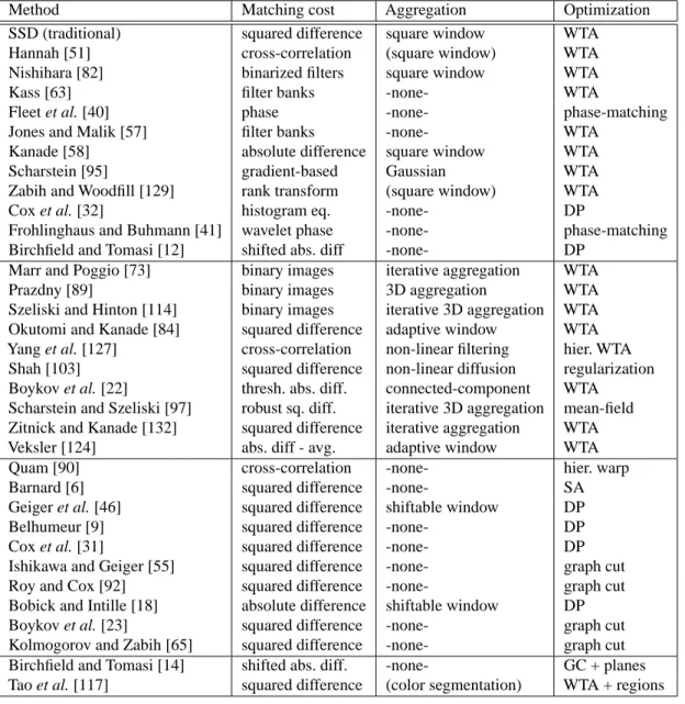
Table 1 gives a summary of some representative stereo matching algorithms and their corresponding taxonomy, i.e., the matching cost, aggregation, and optimization techniques used by each. The methods are grouped to contrast different matching costs (top), aggregation methods (middle), and op-timization techniques (third section), while the last section lists some papers outside the framework. As can be seen from this table, quite a large subset of the possible algorithm design space has been explored over the years, albeit not very systematically.
4. Implementation
We have developed a stand-alone, portable C++ implemen-tation of several stereo algorithms. The implemenimplemen-tation is closely tied to the taxonomy presented in Section 3 and cur-rently includes window-based algorithms, diffusion
algo-Method Matching cost Aggregation Optimization
SSD (traditional) squared difference square window WTA
Hannah [51] cross-correlation (square window) WTA
Nishihara [82] binarized filters square window WTA
Kass [63] filter banks -none- WTA
Fleet et al. [40] phase -none- phase-matching
Jones and Malik [57] filter banks -none- WTA
Kanade [58] absolute difference square window WTA
Scharstein [95] gradient-based Gaussian WTA
Zabih and Woodfill [129] rank transform (square window) WTA
Cox et al. [32] histogram eq. -none- DP
Frohlinghaus and Buhmann [41] wavelet phase -none- phase-matching Birchfield and Tomasi [12] shifted abs. diff -none- DP
Marr and Poggio [73] binary images iterative aggregation WTA
Prazdny [89] binary images 3D aggregation WTA
Szeliski and Hinton [114] binary images iterative 3D aggregation WTA Okutomi and Kanade [84] squared difference adaptive window WTA Yang et al. [127] cross-correlation non-linear filtering hier. WTA Shah [103] squared difference non-linear diffusion regularization Boykov et al. [22] thresh. abs. diff. connected-component WTA Scharstein and Szeliski [97] robust sq. diff. iterative 3D aggregation mean-field Zitnick and Kanade [132] squared difference iterative aggregation WTA
Veksler [124] abs. diff - avg. adaptive window WTA
Quam [90] cross-correlation -none- hier. warp
Barnard [6] squared difference -none- SA
Geiger et al. [46] squared difference shiftable window DP
Belhumeur [9] squared difference -none- DP
Cox et al. [31] squared difference -none- DP
Ishikawa and Geiger [55] squared difference -none- graph cut
Roy and Cox [92] squared difference -none- graph cut
Bobick and Intille [18] absolute difference shiftable window DP
Boykov et al. [23] squared difference -none- graph cut
Kolmogorov and Zabih [65] squared difference -none- graph cut Birchfield and Tomasi [14] shifted abs. diff. -none- GC + planes Tao et al. [117] squared difference (color segmentation) WTA + regions
Table 1: Summary taxonomy of several dense two-frame stereo correspondence methods. The methods are grouped to contrast different
matching costs (top), aggregation methods (middle), and optimization techniques (third section). The last section lists some papers outside our framework. Key to abbreviations: hier. – hierarchical (coarse-to-fine), WTA – winner-take-all, DP – dynamic programming, SA – simulated annealing, GC – graph cut.
rithms, as well as global optimization methods using dy-namic programming, simulated annealing, and graph cuts. While many published methods include special features and post-processing steps to improve the results, we have chosen to implement the basic versions of such algorithms, in order to assess their respective merits most directly.
The implementation is modular and can easily be ex-tended to include other algorithms or their components. We plan to add several other algorithms in the near future, and we hope that other authors will contribute their methods to our framework as well. Once a new algorithm has been inte-grated, it can easily be compared with other algorithms using our evaluation module, which can measure disparity error and reprojection error (Section 5.1). The implementation contains a sophisticated mechanism for specifying parame-ter values that supports recursive script files for exhaustive performance comparisons on multiple data sets.
We provide a high-level description of our code using the same division into four parts as in our taxonomy. Within our code, these four sections are (optionally) executed in sequence, and the performance/quality evaluator is then in-voked. A list of the most important algorithm parameters is given in Table 2.
4.1. Matching cost computation
The simplest possible matching cost is the squared or ab-solute difference in color / intensity between corresponding pixels (match fn). To approximate the effect of a robust matching score [16, 97], we truncate the matching score to a maximal value match max. When color images are being compared, we sum the squared or absolute intensity differ-ence in each channel before applying the clipping. If frac-tional disparity evaluation is being performed (disp step<
1), each scanline is first interpolated up using either a linear or cubic interpolation filter (match interp) [77]. We also optionally apply Birchfield and Tomasi’s sampling insensi-tive interval-based matching criterion (match interval) [12], i.e., we take the minimum of the pixel matching score and the score at±12-step displacements, or 0 if there is a sign change in either interval. We apply this criterion separately to each color channel, which is not physically plausible (the sub-pixel shift must be consistent across channels), but is easier to implement.
4.2. Aggregation
The aggregation section of our test bed implements some commonly used aggregation methods (aggr fn):
• Box filter: use a separable moving average filter (add one right/bottom value, subtract one left/top). This im-plementation trick makes such window-based aggrega-tion insensitive to window size in terms of computaaggrega-tion time and accounts for the fast performance seen in real-time matchers [59, 64].
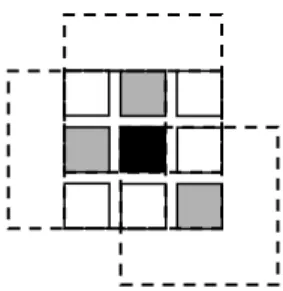
Figure 3: Shiftable window. The effect of trying all3×3shifted windows around the black pixel is the same as taking the minimum matching score across all centered (non-shifted) windows in the same neighborhood. (Only 3 of the neighboring shifted windows are shown here for clarity.)
• Binomial filter: use a separable FIR (finite impulse re-sponse) filter. We use the coefficients1/16{1,4,6,4,1},
the same ones used in Burt and Adelson’s [26] Lapla-cian pyramid.
Other convolution kernels could also be added later, as could recursive (bi-directional) IIR filtering, which is a very efficient way to obtain large window sizes [35]. The width of the box or convolution kernel is controlled by aggr window size.
To simulate the effect of shiftable windows [2, 18, 117], we can follow this aggregation step with a separable square min-filter. The width of this filter is controlled by the param-eter aggr minfilter. The cascaded effect of a box-filter and an equal-sized min-filter is the same as evaluating a complete set of shifted windows, since the value of a shifted window is the same as that of a centered window at some neighboring pixel (Figure 3). This step adds very little additional com-putation, since a moving 1-D min-filter can be computed efficiently by only recomputing the min when a minimum value leaves the window. The value of aggr minfilter can be less than that of aggr window size, which simulates the effect of a partially shifted window. (The converse doesn’t make much sense, since the window then no longer includes the reference pixel.)
We have also implemented all of the diffusion methods developed in [97] except for local stopping, i.e., regular fusion, the membrane model, and Bayesian (mean-field) dif-fusion. While this last algorithm can also be considered an optimization method, we include it in the aggregation mod-ule since it resembles other iterative aggregation algorithms closely. The maximum number of aggregation iterations is controlled by aggr iter. Other parameters controlling the diffusion algorithms are listed in Table 2.
4.3. Optimization
Once we have computed the (optionally aggregated) costs, we need to determine which discrete set of disparities best represents the scene surface. The algorithm used to
deter-Name Typical values Description
disp min 0 smallest disparity
disp max 15 largest disparity
disp step 0.5 disparity step size
match fn SD, AD matching function
match interp Linear, Cubic interpolation function
match max 20 maximum difference for truncated SAD/SSD
match interval false 1/2 disparity match [12] aggr fn Box, Binomial aggregation function
aggr window size 9 size of window
aggr minfilter 9 spatial min-filter (shiftable window)
aggr iter 1 number of aggregation iterations
diff lambda 0.15 parameterλfor regular and membrane diffusion
diff beta 0.5 parameterβfor membrane diffusion
diff scale cost 0.01 scale of cost values (needed for Bayesian diffusion)
diff mu 0.5 parameterµfor Bayesian diffusion
diff sigmaP 0.4 parameterσP for robust prior of Bayesian diffusion diff epsP 0.01 parameterP for robust prior of Bayesian diffusion opt fn WTA, DP, SA, GC optimization function
opt smoothness 1.0 weight of smoothness term (λ)
opt grad thresh 8.0 threshold for magnitude of intensity gradient opt grad penalty 2.0 smoothness penalty factor if gradient is too small opt occlusion cost 20 cost for occluded pixels in DP algorithm
opt sa var Gibbs, Metropolis simulated annealing update rule opt sa start T 10.0 starting temperature
opt sa end T 0.01 ending temperature
opt sa schedule Linear annealing schedule
refine subpix true fit sub-pixel value to local correlation eval bad thresh 1.0 acceptable disparity error
eval textureless width 3 box filter width applied to∇xI2 eval textureless thresh 4.0 threshold applied to filtered∇xI2
eval disp gap 2.0 disparity jump threshold
eval discont width 9 width of discontinuity region eval ignore border 10 number of border pixels to ignore eval partial shuffle 0.2 analysis interval for prediction error
mine this is controlled by opt fn, and can be one of: • winner-take-all (WTA);
• dynamic programming (DP); • scanline optimization (SO); • simulated annealing (SA); • graph cut (GC).
The winner-take-all method simply picks the lowest (aggre-gated) matching cost as the selected disparity at each pixel. The other methods require (in addition to the matching cost) the definition of a smoothness cost. Prior to invoking one of the optimization algorithms, we set up tables containing the values ofρd in Equation (6) and precompute the spa-tially varying weightsρI(x, y). These tables are controlled by the parameters opt smoothness, which controls the over-all scale of the smoothness term (i.e., λin Equation (3)), and the parameters opt grad thresh and opt grad penalty, which control the gradient-dependent smoothness costs. We currently use the smoothness terms defined by Veksler [123]:
ρI(∆I) =
p if ∆I <opt grad thresh
1 if ∆I≥opt grad thresh, (7) wherep =opt grad penalty. Thus, the smoothness cost is multiplied by p for low intensity gradient to encourage disparity jumps to coincide with intensity edges. All of the optimization algorithms minimize the same objective func-tion, enabling a more meaningful comparison of their per-formance.
Our first global optimization technique, DP, is a dynamic programming method similar to the one proposed by Bobick and Intille [18]. The algorithm works by computing the minimum-cost path through eachx-dslice in the DSI (see Figure 2). Every point in this slice can be in one of three states: M (match), L (left-visible only), or R (right-visible only). Assuming the ordering constraint is being enforced, a valid path can take at most three directions at a point, each associated with a deterministic state change. Using dynamic programming, the minimum cost of all paths to a point can be accumulated efficiently. Points in state M are simply charged the matching cost at this point in the DSI. Points in states L and R are charged a fixed occlusion cost (opt occlusion cost). Before evaluating the final disparity map, we fill all occluded pixels with the nearest background disparity value on the same scanline.
The DP stereo algorithm is fairly sensitive to this param-eter (see Section 6). Bobick and Intille address this problem by precomputing ground control points (GCPs) that are then used to constrain the paths through the DSI slice. GCPs are high-confidence matches that are computed using SAD and shiftable windows. At this point we are not using GCPs in our implementation since we are interested in comparing the
basic version of different algorithms. However, GCPs are potentially useful in other algorithms as well, and we plan to add them to our implementation in the future.
Our second global optimization technique, scanline opti-mization (SO), is a simple (and, to our knowledge, novel) ap-proach designed to assess different smoothness terms. Like the previous method, it operates on individualx-dDSI slices and optimizes one scanline at a time. However, the method is asymmetric and does not utilize visibility or ordering con-straints. Instead, advalue is assigned at each pointxsuch that the overall cost along the scanline is minimized. (Note that without a smoothness term, this would be equivalent to a winner-take-all optimization.) The global minimum can again be computed using dynamic programming; however, unlike in traditional (symmetric) DP algorithms, the order-ing constraint does not need to be enforced, and no occlusion cost parameter is necessary. Thus, the SO algorithm solves the same optimization problem as the graph-cut algorithm described below, except that vertical smoothness terms are ignored.
Both DP and SO algorithms suffer from the well-known difficulty of enforcing inter-scanline consistency, resulting in horizontal “streaks” in the computed disparity map. Bo-bick and Intille’s approach to this problem is to detect edges in the DSI slice and to lower the occlusion cost for paths along those edges. This has the effect of aligning depth dis-continuities with intensity edges. In our implementation, we achieve the same goal by using an intensity-dependent smoothness cost (Equation (6)), which, in our DP algorithm, is charged at all L-M and R-M state transitions.
Our implementation of simulated annealing supports both the Metropolis variant (where downhill steps are always taken, and uphill steps are sometimes taken), and the Gibbs Sampler, which chooses among several possible states ac-cording to the full marginal distribution [47]. In the latter case, we can either select one new state (disparity) to flip to at random, or evaluate all possible disparities at a given pixel. Our current annealing schedule is linear, although we plan to add a logarithmic annealing schedule in the future.
Our final global optimization method, GC, implements theα-β swap move algorithm described in [23, 123]. (We plan to implement theα-expansion in the future.) We ran-domize theα-β pairings at each (inner) iteration and stop the algorithm when no further (local) energy improvements are possible.
4.4. Refinement
The sub-pixel refinement of disparities is controlled by the boolean variable refine subpix. When this is enabled, the three aggregated matching cost values around the winning disparity are examined to compute the sub-pixel disparity estimate. (Note that if the initial DSI was formed with frac-tional disparity steps, these are really sub-sub-pixel values. A more appropriate name might be floating point disparity
values.) A parabola is fit to these three values (the three end-ing values are used if the winnend-ing disparity is either disp min or disp max). If the curvature is positive and the minimum of the parabola is within a half-step of the winning disparity (and within the search limits), this value is used as the final disparity estimate.
In future work, we would like to investigate whether initial or aggregated matching scores should be used, or whether some other approach, such as Lucas-Kanade, might yield higher-quality estimates [122].
5. Evaluation methodology
In this section, we describe the quality metrics we use for evaluating the performance of stereo correspondence algo-rithms and the techniques we used for acquiring our image data sets and ground truth estimates.
5.1. Quality metrics
To evaluate the performance of a stereo algorithm or the effects of varying some of its parameters, we need a quan-titative way to estimate the quality of the computed corre-spondences. Two general approaches to this are to compute error statistics with respect to some ground truth data [8] and to evaluate the synthetic images obtained by warping the reference or unseen images by the computed disparity map [111].
In the current version of our software, we compute the following two quality measures based on known ground truth data:
1. RMS (root-mean-squared) error (measured in disparity units) between the computed disparity mapdC(x, y) and the ground truth mapdT(x, y), i.e.,
R=
1
N
(x,y)
|dC(x, y)−dT(x, y)|2 1 2
, (8)
whereNis the total number of pixels. 2. Percentage of bad matching pixels,
B= N1
(x,y)
(|dC(x, y)−dT(x, y)|> δd), (9)
whereδd (eval bad thresh) is a disparity error toler-ance. For the experiments in this paper we useδd = 1.0, since this coincides with some previously published studies [116, 132, 65].
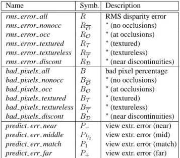
In addition to computing these statistics over the whole image, we also focus on three different kinds of regions. These regions are computed by pre-processing the reference image and ground truth disparity map to yield the following three binary segmentations (Figure 4):
Name Symb. Description
rms error all R RMS disparity error rms error nonocc RO " (no occlusions) rms error occ RO " (at occlusions) rms error textured RT " (textured) rms error textureless RT " (textureless)
rms error discont RD " (near discontinuities) bad pixels all B bad pixel percentage bad pixels nonocc BO " (no occlusions) bad pixels occ BO " (at occlusions) bad pixels textured BT " (textured) bad pixels textureless BT " (textureless)
bad pixels discont BD " (near discontinuities) predict err near P− view extr. error (near) predict err middle P1/
2 view extr. error (mid) predict err match P1 view extr. error (match) predict err far P+ view extr. error (far)
Table 3: Error (quality) statistics computed by our evaluator. See
the notes in the text regarding the treatment of occluded regions.
• textureless regionsT: regions where the squared hor-izontal intensity gradient averaged over a square win-dow of a given size (eval textureless width) is below a given threshold (eval textureless thresh);
• occluded regionsO: regions that are occluded in the matching image, i.e., where the forward-mapped dis-parity lands at a location with a larger (nearer) disdis-parity; and
• depth discontinuity regionsD: pixels whose neighbor-ing disparities differ by more than eval disp gap, di-lated by a window of width eval discont width. These regions were selected to support the analysis of match-ing results in typical problem areas. For the experiments in this paper we use the values listed in Table 2.
The statistics described above are computed for each of the three regions and their complements, e.g.,
BT = N1
T
(x,y)∈T
(|dc(x, y)−dt(x, y)|< δd),
and so on forRT,BT, . . . ,RD.
Table 3 gives a complete list of the statistics we collect. Note that for the textureless, textured, and depth discontinu-ity statistics, we exclude pixels that are in occluded regions, on the assumption that algorithms generally do not pro-duce meaningful results in such occluded regions. Also, we exclude a border of eval ignore border pixels when com-puting all statistics, since many algorithms do not compute meaningful disparities near the image boundaries.
(a) (b)
(c) (d)
Figure 4: Segmented region maps: (a) original image, (b) true disparities, (c) textureless regions (white) and occluded regions (black), (d)
depth discontinuity regions (white) and occluded regions (black).
Figure 5: Series of forward-warped reference images. The reference image is the middle one, the matching image is the second from the
right. Pixels that are invisible (gaps) are shown in light magenta.
Figure 6: Series of inverse-warped original images. The reference image is the middle one, the matching image is the second from the
right. Pixels that are invisible are shown in light magenta. Viewing this sequence (available on our web site) as an animation loop is a good way to check for correct rectification, other misalignments, and quantization effects.
The second major approach to gauging the quality of re-construction algorithms is to use the color images and dis-parity maps to predict the appearance of other views [111]. Here again there are two major flavors possible:
1. Forward warp the reference image by the computed disparity map to a different (potentially unseen) view (Figure 5), and compare it against this new image to obtain a forward prediction error.
2. Inverse warp a new view by the computed disparity map to generate a stabilized image (Figure 6), and compare it against the reference image to obtain an inverse pre-diction error.
There are pros and cons to either approach.
The forward warping algorithm has to deal with tearing problems: if a single-pixel splat is used, gaps can arise even between adjacent pixels with similar disparities. One pos-sible solution would be to use a two-pass renderer [102]. Instead, we render each pair of neighboring pixel as an in-terpolated color line in the destination image (i.e., we use Gouraud shading). If neighboring pixels differ by more that a disparity of eval disp gap, the segment is replaced by sin-gle pixel spats at both ends, which results in a visible tear (light magenta regions in Figure 5).
For inverse warping, the problem of gaps does not oc-cur. Instead, we get “ghosted” regions when pixels in the reference image are not actually visible in the source. We eliminate such pixels by checking for visibility (occlusions) first, and then drawing these pixels in a special color (light magenta in Figure 6). We have found that looking at the inverse warped sequence, based on the ground-truth dispari-ties, is a very good way to determine if the original sequence is properly calibrated and rectified.
In computing the prediction error, we need to decide how to treat gaps. Currently, we ignore pixels flagged as gaps in computing the statistics and report the percentage of such missing pixels. We can also optionally compensate for small misregistrations [111]. To do this, we convert each pixel in the original and predicted image to an interval, by blend-ing the pixel’s value with some fraction eval partial shuffle of its neighboring pixels min and max values. This idea is a generalization of the sampling-insensitive dissimilarity measure [12] and the shuffle transformation of [66]. The reported difference is then the (signed) distance between the two computed intervals. We plan to investigate these and other sampling-insensitive matching costs in the future [115].
5.2. Test data
To quantitatively evaluate our correspondence algorithms, we require data sets that either have a ground truth dispar-ity map, or a set of additional views that can be used for prediction error test (or preferably both).
We have begun to collect such a database of images, build-ing upon the methodology introduced in [116]. Each image sequence consists of 9 images, taken at regular intervals with a camera mounted on a horizontal translation stage, with the camera pointing perpendicularly to the direction of motion. We use a digital high-resolution camera (Canon G1) set in manual exposure and focus mode and rectify the images us-ing tracked feature points. We then downsample the original
2048×1536images to512×384using a high-quality 8-tap filter and finally crop the images to normalize the motion of background objects to a few pixels per frame.
All of the sequences we have captured are made up of piecewise planar objects (typically posters or paintings, some with cut-out edges). Before downsampling the images, we hand-label each image into its piecewise planar compo-nents (Figure 7). We then use a direct alignment technique on each planar region [5] to estimate the affine motion of each patch. The horizontal component of these motions is then used to compute the ground truth disparity. In future work we plan to extend our acquisition methodology to han-dle scenes with quadric surfaces (e.g., cylinders, cones, and spheres).
Of the six image sequences we acquired, all of which are available on our web page, we have selected two (“Sawtooth” and “Venus”) for the experimental study in this paper. We also use the University of Tsukuba “head and lamp” data set [81], a5×5array of images together with hand-labeled integer ground-truth disparities for the center image. Finally, we use the monochromatic “Map” data set first introduced by Szeliski and Zabih [116], which was taken with a Point Grey Research trinocular stereo camera, and whose ground-truth disparity map was computed using the piecewise planar technique described above. Figure 7 shows the reference image and the ground-truth disparities for each of these four sequences. We exclude a border of 18 pixels in the Tsukuba images, since no ground-truth disparity values are provided there. For all other images, we use eval ignore border= 10 for the experiments reported in this paper.
In the future, we hope to add further data sets to our collection of “standard” test images, in particular other se-quences from the University of Tsukuba, and the GRASP Laboratory’s “Buffalo Bill” data set with registered laser range finder ground truth [80]. There may also be suitable images among the CMU Computer Vision Home Page data sets. Unfortunately, we cannot use data sets for which only a sparse set of feature matches has been computed [19, 54]. It should be noted that high-quality ground-truth data is critical for a meaningful performance evaluation. Accurate sub-pixel disparities are hard to come by, however. The ground-truth data for the Tsukuba images, for example, is strongly quantized since it only provides integer disparity estimates for a very small disparity range (d = 5. . .14). This is clearly visible when the images are stabilized using
Sawtooth ref. image planar regions ground-truth disparities
Venus ref. image planar regions ground-truth disparities
Tsukuba ref. image ground-truth disparities
Map ref. image ground-truth disparities
Figure 7: Stereo images with ground truth used in this study. The Sawtooth and Venus images are two of our new 9-frame stereo sequences
of planar objects. The figure shows the reference image, the planar region labeling, and the ground-truth disparities. We also use the familiar Tsukuba “head and lamp” data set, and the monochromatic Map image pair.
the ground-truth data and viewed in a video loop. In contrast, the ground-truth disparities for our piecewise planar scenes have high (subpixel) precision, but at the cost of limited scene complexity. To provide an adequate challenge for the best-performing stereo methods, new stereo test images with complex scenes and sub-pixel ground truth will soon be needed.
Synthetic images have been used extensively for quali-tative evaluations of stereo methods, but they are often re-stricted to simple geometries and textures (e.g., random-dot stereograms). Furthermore, issues arising with real cam-eras are seldom modeled, e.g., aliasing, slight misalignment, noise, lens aberrations, and fluctuations in gain and bias. Consequently, results on synthetic images usually do not extrapolate to images taken with real cameras. We have experimented with the University of Bonn’s synthetic “Cor-ridor” data set [41], but have found that the clean, noise-free images are unrealistically easy to solve, while the noise-contaminated versions are too difficult due to the complete lack of texture in much of the scene. There is a clear need for synthetic, photo-realistic test imagery that properly models real-world imperfections, while providing accurate ground truth.
6. Experiments and results
In this section, we describe the experiments used to evalu-ate the individual building blocks of stereo algorithms. Us-ing our implementation framework, we examine the four main algorithm components identified in Section 3 (match-ing cost, aggregation, optimization, and sub-pixel fitt(match-ing) In Section 7, we perform an overall comparison of a large set of stereo algorithms, including other authors’ implemen-tations. We use the Tsukuba, Sawtooth, Venus, and Map data sets in all experiments and report results on subsets of these images. The complete set of results (all experi-ments run on all data sets) is available on our web site at
www.middlebury.edu/stereo.
Using the evaluation measures presented in Section 5.1, we focus on common problem areas for stereo algorithms. Of the 12 ground-truth statistics we collect (Table 3), we have chosen three as the most important subset. First, as a measure of overall performance, we useBO, the percent-age of bad pixels in non-occluded areas. We exclude the occluded regions for now since few of the algorithms in this study explicitly model occlusions, and most perform quite poorly in these regions. As algorithms get better at matching occluded regions [65], however, we will likely focus more on the total matching errorB.
The other two important measures areBT andBD, the percentage of bad pixels in textureless areas and in areas near depth discontinuities. These measures provide important in-formation about the performance of algorithms in two criti-cal problem areas. The parameter names for these three
mea-sures are bad pixels nonocc, bad pixels textureless, and bad pixels discont, and they appear in most of the plots below. We prefer the percentage of bad pixels over RMS disparity errors since this gives a better indication of the overall performance of an algorithm. For example, an al-gorithm is performing reasonably well ifBO <10%. The RMS error figure, on the other hand, is contaminated by the (potentially large) disparity errors in those poorly matched
10%of the image. RMS errors become important once the percentage of bad pixels drops to a few percent and the qual-ity of a sub-pixel fit needs to be evaluated (see Section 6.4). Note that the algorithms always take exactly two images as input, even when more are available. For example, with our 9-frame sequences, we use the third and seventh frame as input pair. (The other frames are used to measure the prediction error.)
6.1. Matching cost
We start by comparing different matching costs, including absolute differences (AD), squared differences (SD), trun-cated versions of both, and Birchfield and Tomasi’s [12] sampling-insensitive dissimilarity measure (BT).
An interesting issue when trying to assess a single algo-rithm component is how to fix the parameters that control the other components. We usually choose good values based on experiments that assess the other algorithm components. (The inherent boot-strapping problem disappears after a few rounds of experiments.) Since the best settings for many pa-rameters vary depending on the input image pair, we often have to compromise and select a value that works reasonably well for several images.
Experiment 1: In this experiment we compare the
match-ing costs AD, SD, AD+BT, and SD+BT usmatch-ing a local al-gorithm. We aggregate with a9×9 window, followed by winner-take-all optimization (i.e., we use the standard SAD and SSD algorithms). We do not compute sub-pixel esti-mates. Truncation values used are 1, 2, 5, 10, 20, 50, and ∞(no truncation); these values are squared when truncating SD.
Results: Figure 8 shows plots of the three evaluation
mea-suresBO,BT, andBD for each of the four matching costs as a function of truncation values, for the Tsukuba, Saw-tooth, and Venus images. Overall, there is little difference between AD and SD. Truncation matters mostly for points near discontinuities. The reason is that for windows con-taining mixed populations (both foreground and background points), truncating the matching cost limits the influence of wrong matches. Good truncation values range from 5 to 50, typically around 20. Once the truncation values drop below the noise level (e.g., 2 and 1), the errors become very large. Using Birchfield-Tomasi (BT) helps for these small trunca-tion values, but yields little improvement for good truncatrunca-tion
Tsukuba 9x9
0% 10% 20% 30% 40% 50% 60%
in
f
50 20 10 5 2 1 inf 50 20 10 5 2 1 fin 50 20 10 5 2 1 inf 50 20 10 5 2 1
SAD SSD SAD+BT SSD+BT
match_max
bad_pixels_nonocc bad_pixels_textureless bad_pixels_discont
Sawtooth 9x9
0% 10% 20% 30% 40% 50% 60%
in
f
50 20 10 5 2 1 inf 50 20 10 5 2 1 fin 50 20 10 5 2 1 inf 50 20 10 5 2 1
SAD SSD SAD+BT SSD+BT
match_max
bad_pixels_nonocc bad_pixels_textureless bad_pixels_discont
Venus 9x9
0% 10% 20% 30% 40% 50% 60%
in
f
50 20 10 5 2 1 inf 50 20 10 5 2 1 fin 50 20 10 5 2 1 inf 50 20 10 5 2 1
SAD SSD SAD+BT SSD+BT
match_max
bad_pixels_nonocc bad_pixels_textureless bad_pixels_discont
Figure 8: Experiment 1. Performance of different matching costs aggregated with a9×9window as a function of truncation values
match max for three different image pairs. Intermediate truncation values (5–20) yield the best results. Birchfield-Tomasi (BT) helps when
values. The results are consistent across all data sets; how-ever, the best truncation value varies. We have also tried a window size of 21, with similar results.
Conclusion: Truncation can help for AD and SD, but the
best truncation value depends on the images’signal-to-noise-ratio (SNR), since truncation should happen right above the noise level present (see also the discussion in [97]).
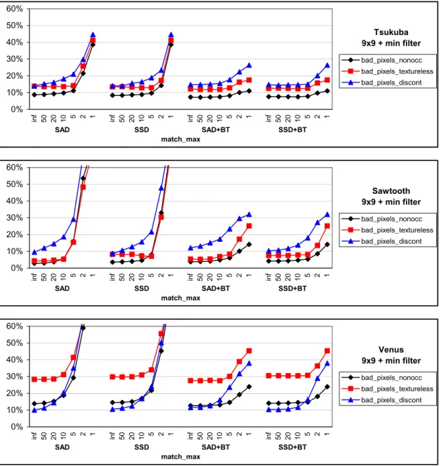
Experiment 2: This experiment is identical to the
previ-ous one, except that we also use a9×9min-filter (in effect, we aggregate with shiftable windows).
Results: Figure 9 shows the plots for this experiment, again
for Tsukuba, Sawtooth, and Venus images. As before, there are negligible differences between AD and SD. Now, how-ever, the non-truncated versions perform consistently the best. In particular, for points near discontinuities we get the lowest errors overall, but also the total errors are com-parable to the best settings of truncation in Experiment 1. BT helps bring down larger errors, but as before, does not significantly decrease the best (non-truncated) errors. We again also tried a window size of 21 with similar results.
Conclusion: The problem of selecting the best truncation
value can be avoided by instead using a shiftable window (min-filter). This is an interesting result, as both robust matching costs (trunctated functions) and shiftable windows have been proposed to deal with outliers in windows that straddle object boundaries. The above experiments suggest that avoiding outliers by shifting the window is preferable to limiting their influence using truncated cost functions.
Experiment 3: We now assess how matching costs affect
global algorithms, using dynamic programming (DP), scan-line optimization (SO), and graph cuts (GC) as optimization techniques. A problem with global techniques that minimize a weighted sum of data and smoothness terms (Equation (3)) is that the range of matching cost values affects the optimal value forλ, i.e., the relative weight of the smoothness term. For example, squared differences require much higher values forλthan absolute differences. Similarly, truncated differ-ence functions result in lower matching costs and require lower values forλ. Thus, in trying to isolate the effect of the matching costs, we are faced with the problem of how to chooseλ. The cleanest solution to this dilemma would per-haps be to find a (different) optimalλindependently for each matching cost under consideration, and then to report which matching cost gives the overall best results. The optimalλ, however, would not only differ across matching costs, but also across different images. Since in a practical matcher we need to choose a constantλ, we have done the same in this experiment. We useλ= 20(guided by the results dis-cussed in Section 6.3 below) and restrict the matching costs to absolute differences (AD), truncated by varying amounts. For the DP algorithm we use a fixed occlusion cost of 20.
Results: Figure 10 shows plots of the bad pixel
percent-agesBO,BT, andBD as a function of truncation values for Tsukuba, Sawtooth, and Venus images. Each plot has six curves, corresponding to DP, DP+BT, SO, SO+BT, GC, GC+BT. It can be seen that the truncation value affects the performance. As with the local algorithms, if the truncation value is too small (in the noise range), the errors get very large. Intermediate truncation values of 50–5, depending on algorithm and image pair, however, can sometimes improve the performance. The effect of Birchfield-Tomasi is mixed; as with the local algorithms in Experiments 1 and 2, it limits the errors if the truncation values are too small. It can be seen that BT is most beneficial for the SO algorithm, how-ever, this is due to the fact that SO really requires a higher value ofλto work well (see Experiment 5), in which case the positive effect of BT is less pronounced.
Conclusion: Using robust (truncated) matching costs can
slightly improve the performance of global algorithms. The best truncation value, however, varies with each image pair. Setting this parameter automatically based on an estimate of the image SNR may be possible and is a topic for fur-ther research. Birchfield and Tomasi’s matching measure can improve results slightly. Intuitively, truncation should not be necessary for global algorithms that operate on un-aggregated matching costs, since the problem of outliers in a window does not exist. An important problem for global algorithms, however, is to find the correct balance between data and smoothness terms (see Experiment 5 below). Trun-cation can be useful in this context since it limits the range of possible cost values.
6.2. Aggregation
We now turn to comparing different aggregation methods used by local methods. While global methods typically op-erate on raw (unaggregated) costs, aggregation can be useful for those methods as well, for example to provide starting values for iterative algorithms, or a set of high-confidence matches or ground control points (GCPs) [18] used to restrict the search of dynamic-programming methods.
In this section we examine aggregation with square win-dows, shiftable windows (min-filter), binomial filters, reg-ular diffusion, and membrane diffusion [97]. Results for Bayesian diffusion, which combines aggregation and opti-mization, can be found in Section 7.
Experiment 4: In this experiment we use (non-truncated)
absolute differences as matching cost and perform a winner-take-all optimization after the aggregation step (no sub-pixel estimation). We compare the following aggregation meth-ods:
1. square windows with window sizes 3, 5, 7, . . . , 29; 2. shiftable square windows (min-filter) with window
Tsukuba 9x9 + min filter
0% 10% 20% 30% 40% 50% 60%
in
f
50 20 10 5 2 1 inf 50 20 10 5 2 1 fin 50 20 10 5 2 1 inf 50 20 10 5 2 1
SAD SSD SAD+BT SSD+BT
match_max
bad_pixels_nonocc bad_pixels_textureless bad_pixels_discont
Sawtooth 9x9 + min filter
0% 10% 20% 30% 40% 50% 60%
in
f
50 20 10 5 2 1 inf 50 20 10 5 2 1 fin 50 20 10 5 2 1 inf 50 20 10 5 2 1
SAD SSD SAD+BT SSD+BT
match_max
bad_pixels_nonocc bad_pixels_textureless bad_pixels_discont
Venus 9x9 + min filter
0% 10% 20% 30% 40% 50% 60%
in
f
50 20 10 5 2 1 inf 50 20 10 5 2 1 fin 50 20 10 5 2 1 inf 50 20 10 5 2 1
SAD SSD SAD+BT SSD+BT
match_max
bad_pixels_nonocc bad_pixels_textureless bad_pixels_discont
Figure 9: Experiment 2. Performance of different matching costs aggregated with a9×9shiftable window (min-filter) as a function of truncation values match max for three different image pairs. Large truncation values (no truncation) work best when using shiftable windows.
Tsukuba
0% 10% 20% 30% 40% 50% 60%
in
f
50 20 10 5 2 inf 50 20 10 5 2 inf 50 20 10 5 2 inf 50 20 10 5 2 inf 50 20 10 5 inf 50 20 10 5
DP DP+BT SO SO+BT GC GC+BT
match_max
bad_pixels_nonocc bad_pixels_textureless bad_pixels_discont
Sawtooth
0% 10% 20% 30% 40% 50% 60%
in
f
50 20 10 5 2 inf 50 20 10 5 2 inf 50 20 10 5 2 inf 50 20 10 5 2 inf 50 20 10 5 inf 50 20 10 5
DP DP+BT SO SO+BT GC GC+BT
match_max
bad_pixels_nonocc bad_pixels_textureless bad_pixels_discont
Venus
0% 10% 20% 30% 40% 50% 60%
in
f
50 20 10 5 2 inf 50 20 10 5 2 inf 50 20 10 5 2 inf 50 20 10 5 2 inf 50 20 10 5 inf 50 20 10 5
DP DP+BT SO SO+BT GC GC+BT
match_max
bad_pixels_nonocc bad_pixels_textureless bad_pixels_discont
Figure 10: Experiment 3. Performance of different matching costs for global algorithms as a function of truncation values match max for