JCGM 102:2011. October 2011

(1)

JCGM 102

:

2011

Evaluation of measurement

data – Supplement 2 to the

“Guide to the expression of

uncertainty in measurement” –

Extension to any number of

output quantities

Évaluation des données de mesure

−

Supplément 2 du “Guide pour

l’expression de l’incertitude de mesure”

– Extension à un nombre quelconque de

grandeurs de sortie

October 2011

(2)

Document produced by Working Group 1 of the Joint Committee for Guides in Metrology (JCGM/WG 1).

Copyright of this document is shared jointly by the JCGM member organizations (BIPM, IEC, IFCC, ILAC, ISO, IUPAC, IUPAP and OIML).

Document produit par le Groupe de travail 1 du Comité commun pour les guides en métrologie (JCGM/WG 1).

Les droits d’auteur relatifs à ce document sont la propriété conjointe des organisations membres du JCGM (BIPM, CEI, IFCC, ILAC, ISO, IUPAC, IUPAP et OIML).

Copyrights

Even if the electronic version of this document is available free of charge on the BIPM’s website (www.bipm.org), copyright of this document is shared jointly by the JCGM member organizations, and all respective logos and emblems are vested in them and are internationally protected. Third parties cannot rewrite or re-brand, issue or sell copies to the public, broadcast or use it on-line. For all commercial use, reproduction or translation of this document and/or of the logos, emblems, publications or other creations contained therein, the prior written permission of the Director of the BIPM must be obtained.

Droits d’auteur

Même si une version électronique de ce document peut être téléchargée gratuitement sur le site internet du BIPM (www.bipm.org), les droits d’auteur relatifs à ce document sont la propriété conjointe des organisations membres du JCGM et l’ensemble de leurs logos et emblèmes respectifs leur appartiennent et font l’objet d’une protection internationale. Les tiers ne peuvent le réécrire ou le modifier, le distribuer ou vendre des copies au public, le diffuser ou le mettre en ligne. Tout usage commercial, reproduction ou traduction de ce document et/ou des logos, emblèmes et/ou publications qu’il comporte, doit recevoir l’autorisation écrite préalable du directeur du BIPM.

(3)

2011

Evaluation of measurement data — Supplement 2

to the “Guide to the expression of uncertainty in

measurement” — Extension to any number of

output quantities

´

Evaluation des donn´

ees de mesure — Suppl´

ement 2 du “Guide pour l’expression

de l’incertitude de mesure” — Extension `

a un nombre quelconque de grandeurs

de sortie

(4)

c

JCGM 2011

Copyright of this JCGM guidance document is shared jointly by the JCGM member organizations (BIPM, IEC, IFCC, ILAC, ISO, IUPAC, IUPAP and OIML).

Copyright

Even if electronic versions are available free of charge on the website of one or more of the JCGM member organizations, economic and moral copyrights related to all JCGM publications are internationally protected. The JCGM does not, without its written authorisation, permit third parties to rewrite or re-brand issues, to sell copies to the public, or to broadcast or use on-line its publications. Equally, the JCGM also objects to distortion, augmentation or mutilation of its publications, including its titles, slogans and logos, and those of its member organizations.

Official versions and translations

The only official versions of documents are those published by the JCGM, in their original languages.

The JCGM’s publications may be translated into languages other than those in which the documents were originally published by the JCGM. Permission must be obtained from the JCGM before a translation can be made. All translations should respect the original and official format of the formulæ and units (without any conversion to other formulæ or units), and contain the following statement (to be translated into the chosen language):

All JCGM’s products are internationally protected by copyright. This translation of the original JCGM document has been produced with the permission of the JCGM. The JCGM retains full internationally protected copyright on the design and content of this document and on the JCGM’s titles, slogan and logos. The member organizations of the JCGM also retain full internationally protected right on their titles, slogans and logos included in the JCGM’s publications. The only official version is the document published by the JCGM, in the original languages.

The JCGM does not accept any liability for the relevance, accuracy, completeness or quality of the information and materials offered in any translation. A copy of the translation shall be provided to the JCGM at the time of publication.

Reproduction

The JCGM’s publications may be reproduced, provided written permission has been granted by the JCGM. A sample of any reproduced document shall be provided to the JCGM at the time of reproduction and contain the following statement:

This document is reproduced with the permission of the JCGM, which retains full internationally protected copyright on the design and content of this document and on the JCGM’s titles, slogans and logos. The member organizations of the JCGM also retain full internationally protected right on their titles, slogans and logos included in the JCGM’s publications. The only official versions are the original versions of the documents published by the JCGM.

Disclaimer

The JCGM and its member organizations have published this document to enhance access to information about metrology. They endeavor to update it on a regular basis, but cannot guarantee the accuracy at all times and shall not be responsible for any direct or indirect damage that may result from its use. Any reference to commercial products of any kind (including but not restricted to any software, data or hardware) or links to websites, over which the JCGM and its member organizations have no control and for which they assume no responsibility, does not imply any approval, endorsement or recommendation by the JCGM and its member organizations.

(5)

Annexes

A (informative) Derivatives of complex multivariate measurement functions . . . 59

B (informative) Evaluation of sensitivity coefficients and covariance matrix for multivariate measurement models. . . 61

C (informative) Co-ordinate system transformation . . . 62

C.1 General . . . 62

C.2 Analytical solution for a special case . . . 62

C.3 Application of the GUM uncertainty framework . . . 64

D (informative) Glossary of principal symbols . . . 65

Bibliography. . . 69

(7)

Foreword

In 1997 a Joint Committee for Guides in Metrology (JCGM), chaired by the Director of the Bureau International des Poids et Mesures (BIPM), was created by the seven international organizations that had originally in 1993 prepared the “Guide to the expression of uncertainty in measurement” (GUM) and the “International vocabulary of basic and general terms in metrology” (VIM). The JCGM assumed responsibility for these two documents from the ISO Technical Advisory Group 4 (TAG4).

The Joint Committee is formed by the BIPM with the International Electrotechnical Commission (IEC), the International Federation of Clinical Chemistry and Laboratory Medicine (IFCC), the International Laboratory Accreditation Cooperation (ILAC), the International Organization for Standardization (ISO), the International Union of Pure and Applied Chemistry (IUPAC), the International Union of Pure and Applied Physics (IUPAP), and the International Organization of Legal Metrology (OIML).

JCGM has two Working Groups. Working Group 1, “Expression of uncertainty in measurement”, has the task to promote the use of the GUM and to prepare Supplements and other documents for its broad application. Working Group 2, “Working Group on International vocabulary of basic and general terms in metrology (VIM)”, has the task to revise and promote the use of the VIM.

Supplements such as this one are intended to give added value to the GUM by providing guidance on aspects of uncertainty evaluation that are not explicitly treated in the GUM. The guidance will, however, be as consistent as possible with the general probabilistic basis of the GUM.

The present Supplement 2 to the GUM has been prepared by Working Group 1 of the JCGM, and has benefited from detailed reviews undertaken by member organizations of the JCGM and National Metrology Institutes.

(8)

Introduction

The “Guide to the expression of uncertainty in measurement” (GUM) [JCGM 100:2008] is mainly concerned with univariate measurement models, namely models having a single scalar output quantity. However, mod-els with more than one output quantity arise across metrology. The GUM includes examples, from electrical metrology, with three output quantities [JCGM 100:2008 H.2], and thermal metrology, with two output quan-tities [JCGM 100:2008 H.3]. This Supplement to the GUM treats multivariate measurement models, namely models with any number of output quantities. Such quantities are generally mutually correlated because they depend on common input quantities. A generalization of the GUM uncertainty framework [JCGM 100:2008 5] is used to provide estimates of the output quantities, the standard uncertainties associated with the estimates, and covariances associated with pairs of estimates. The input or output quantities in the measurement model may be real or complex.

Supplement 1 to the GUM [JCGM 101:2008] is concerned with the propagation of probability distributions [JCGM 101:2008 5] through a measurement model as a basis for the evaluation of measurement uncertainty, and its implementation by a Monte Carlo method [JCGM 101:2008 7]. Like the GUM, it is only concerned with models having a single scalar output quantity [JCGM 101:2008 1]. This Supplement describes a generalization of that Monte Carlo method to obtain a discrete representation of the joint probability distribution for the output quantities of a multivariate model. The discrete representation is then used to provide estimates of the output quantities, and standard uncertainties and covariances associated with those estimates. Appropriate use of the Monte Carlo method would be expected to provide valid results when the applicability of the GUM uncertainty framework is questionable, namely when (a) linearization of the model provides an inadequate representation, or (b) the probability distribution for the output quantity (or quantities) departs appreciably from a (multivariate) Gaussian distribution.

Guidance is also given on the determination of a coverage region for the output quantities of a multivariate model, the counterpart of a coverage interval for a single scalar output quantity, corresponding to a stipulated coverage probability. The guidance includes the provision of coverage regions that take the form of hyper-ellipsoids and hyper-rectangles. A calculation procedure that uses results provided by the Monte Carlo method is also described for obtaining an approximation to the smallest coverage region.

(9)

Evaluation of measurement data — Supplement 2

to the “Guide to the expression of uncertainty in

measurement” — Extension to any number of output

quantities

1 Scope

This Supplement to the “Guide to the expression of uncertainty in measurement” (GUM) is concerned with measurement models having any number of input quantities (as in the GUM and GUM Supplement 1) and any number of output quantities. The quantities involved might be real or complex. Two approaches are considered for treating such models. The first approach is a generalization of the GUM uncertainty framework. The second is a Monte Carlo method as an implementation of the propagation of distributions. Appropriate use of the Monte Carlo method would be expected to provide valid results when the applicability of the GUM uncertainty framework is questionable.

The approach based on the GUM uncertainty framework is applicable when the input quantities are summarized (as in the GUM) in terms of estimates (for instance, measured values) and standard uncertainties associated with these estimates and, when appropriate, covariances associated with pairs of these estimates. Formulæ and procedures are provided for obtaining estimates of the output quantities and for evaluating the associated standard uncertainties and covariances. Variants of the formulæ and procedures relate to models for which the output quantities (a) can be expressed directly in terms of the input quantities as measurement functions, and (b) are obtained through solving a measurement model, which links implicitly the input and output quantities. The counterparts of the formulæ in the GUM for the standard uncertainty associated with an estimate of the output quantity would be algebraically cumbersome. Such formulæ are provided in a more compact form in terms of matrices and vectors, the elements of which contain variances (squared standard uncertainties), covariances and sensitivity coefficients. An advantage of this form of presentation is that these formulæ can readily be implemented in the many computer languages and systems that support matrix algebra.

The Monte Carlo method is based on (i) the assignment of probability distributions to the input quantities in the measurement model [JCGM 101:2008 6], (ii) the determination of a discrete representation of the (joint) probability distribution for the output quantities, and (iii) the determination from this discrete representation of estimates of the output quantities and the evaluation of the associated standard uncertainties and covariances. This approach constitutes a generalization of the Monte Carlo method in Supplement 1 to the GUM, which applies to a single scalar output quantity.

For a prescribed coverage probability, this Supplement can be used to provide a coverage region for the output quantities of a multivariate model, the counterpart of a coverage interval for a single scalar output quantity. The provision of coverage regions includes those taking the form of a hyper-ellipsoid or a hyper-rectangle. These coverage regions are produced from the results of the two approaches described here. A procedure for providing an approximation to the smallest coverage region, obtained from results provided by the Monte Carlo method, is also given.

This Supplement contains detailed examples to illustrate the guidance provided.

This document is a Supplement to the GUM and is to be used in conjunction with it and GUM Supplement 1. The audience of this Supplement is that of the GUM and its Supplements. Also see JCGM 104.

(10)

2 Normative references

The following referenced documents are indispensable for the application of this document. For dated references, only the edition cited applies. For undated references, the latest edition of the referenced document (including any amendments) applies.

JCGM 100:2008. Guide to the expression of uncertainty in measurement (GUM).

JCGM 101:2008. Evaluation of measurement data — Supplement 1 to the “Guide to the expression of uncer-tainty in measurement” — Propagation of distributions using a Monte Carlo method.

JCGM 104:2009. Evaluation of measurement data — An introduction to the “Guide to the expression of uncertainty in measurement” and related documents.

JCGM 200:2008. International Vocabulary of Metrology—Basic and General Concepts and Associated Terms (VIM).

3 Terms and definitions

For the purposes of this Supplement, the definitions of the GUM and the VIM apply unless otherwise indicated. Some of the most relevant definitions, adapted or generalized where necessary from these documents, are given below. Further definitions are given, including definitions taken or adapted from other sources, that are especially important for this Supplement.

A glossary of principal symbols used is given in annex D.

3.1

real quantity

quantity whose numerical value is a real number

3.2

complex quantity

quantity whose numerical value is a complex number

NOTE A complex quantityZcan be represented by two real quantities in Cartesian form

Z≡(ZR, ZI)

>

=ZR+ iZI,

where >denotes “transpose”, i2 =−1 andZR andZI are, respectively, the real and imaginary parts ofZ, or in polar form

Z≡(Zr, Zθ)

>

=Zr(cosZθ+ i sinZθ) =ZreiZθ,

whereZr andZθ are, respectively, the magnitude (amplitude) and phase ofZ. 3.3

vector quantity

set of quantities arranged as a matrix having a single column

3.4

real vector quantity

vector quantity with real components

EXAMPLE A real vector quantityXcontainingNreal quantitiesX1, . . . , XNexpressed as a matrix of dimensionN×1:

X =

  

X1 . . . XN

 

= (X1, . . . , XN) >

(11)

3.5

complex vector quantity

vector quantity with complex components

EXAMPLE A complex vector quantity Z containing N complex quantities Z1, . . . ,ZN expressed as a matrix of

dimensionN×1:

Z=

  

Z1 . . .

ZN

 

= (Z1, . . . ,ZN) >

.

3.6

vector measurand

vector quantity intended to be measured

NOTE Generalized from JCGM 200:2008 definition 2.3.

3.7

measurement model

model of measurement model

mathematical relation among all quantities known to be involved in a measurement

NOTE 1 Adapted from JCGM 200:2008 definition 2.48.

NOTE 2 A general form of a measurement model is the equationh(Y, X1, . . . , XN) = 0, whereY, the output quantity

in the measurement model, is the measurand, the quantity value of which is to be inferred from information about input quantitiesX1, . . . , XN in the measurement model.

NOTE 3 In cases where there are two or more output quantities in a measurement model, the measurement model consists of more than one equation.

3.8

multivariate measurement model

multivariate model

measurement model in which there is any number of output quantities

NOTE 1 The general form of a multivariate measurement model is the equations

h1(Y1, . . . , Ym, X1, . . . , XN) = 0, . . . , hm(Y1, . . . , Ym, X1, . . . , XN) = 0,

whereY1, . . . , Ym, the output quantities,min number, in the multivariate measurement model, constitute the measurand,

the quantity values of which are to be inferred from information about input quantitiesX1, . . . , XN in the multivariate

measurement model.

NOTE 2 A vector representation of the general form of multivariate measurement model is

h(Y,X) =0,

whereY = (Y1, . . . , Ym)>andh= (h1, . . . , hm)>are matrices of dimensionm×1.

NOTE 3 If, in note 1,m, the number of output quantities, is unity, the model is known as a univariate measurement model.

3.9

multivariate measurement function

multivariate function

function in a multivariate measurement model for which the output quantities are expressed in terms of the input quantities

(12)

NOTE 2 If a measurement model h(Y,X) =0can explicitly be written asY =f(X), whereX= (X1, . . . , XN)>

are the input quantities, andY = (Y1, . . . , Ym)>are the output quantities,f = (f1, . . . , fm)>is the multivariate

mea-surement function. More generally,f may symbolize an algorithm, yielding for input quantity valuesx= (x1, . . . , xN)>

a corresponding unique set of output quantity valuesy1=f1(x), . . . , ym=fm(x).

NOTE 3 If, in note 2,m, the number of output quantities, is unity, the function is known as a univariate measurement function.

3.10

real measurement model

real model

measurement model, generally multivariate, involving real quantities

3.11

complex measurement model

complex model

measurement model, generally multivariate, involving complex quantities

3.12

multistage measurement model

multistage model

measurement model, generally multivariate, consisting of a sequence of sub-models, in which output quantities from one sub-model become input quantities to a subsequent sub-model

NOTE Only at the final stage of a multistage measurement model might it be necessary to consider a coverage region for the output quantities based on the joint probability density function for those quantities.

EXAMPLE A common instance in metrology is the following pair of measurement sub-models in the context of cali-bration. The first sub-model has input quantities whose measured values are provided by measurement standards and corresponding indication values, and as output quantities the parameters in a calibration function. This sub-model specifies the manner in which the output quantities are obtained from the input quantities, for example by solving a least-squares problem. The second sub-model has as input quantities the parameters in the calibration function and a quantity realized by a further indication value and as output quantity the quantity corresponding to that input quantity.

3.13

joint distribution function

distribution function

function giving, for every valueξ= (ξ1, . . . , ξN)>, the probability that each elementXiof the random variableX

be less than or equal toξi

NOTE The joint distribution for the random variableX is denoted byGX(ξ), where

GX(ξ) = Pr(X1≤ξ1, . . . , XN≤ξN). 3.14

joint probability density function

probability density function

non-negative functiong_X(ξ) satisfying G_X(ξ) =

Z ξ1

−∞

· · · Z ξN

−∞

g_X(z) dzN· · ·dz1

3.15

marginal probability density function

for a random variableXi, a component ofX having probability density functiongX(ξ), the probability density

function for Xi alone:

g_X

i(ξi) =

Z ∞

−∞

· · · Z ∞

−∞

(13)

NOTE When the componentsXi ofX are independent,gX(ξ) =gX1(ξ1)gX2(ξ2)· · ·gXN(ξN).

3.16

expectation

property of a random variableXi, a component ofX having probability density functiongX(ξ), given by E(Xi) =

Z ∞

−∞

· · · Z ∞

−∞

ξigX(ξ) dξN· · ·dξ1=

Z ∞

−∞

ξigXi(ξi) dξi

NOTE 1 Generalized from JCGM 101:2008 definition 3.6.

NOTE 2 The expectation of the random variableX isE(X) = (E(X1), . . . , E(XN))>, a matrix of dimensionN×1. 3.17

variance

property of a random variableXi, a component ofX having probability density functiongX(ξ), given by V(Xi) =

Z ∞

−∞

· · · Z ∞

−∞

[ξi−E(Xi)]2gX(ξ) dξN· · ·dξ1=

Z ∞

−∞

[ξi−E(Xi)]2gXi(ξi) dξi

NOTE Generalized from JCGM 101:2008 definition 3.7.

3.18 covariance

property of a pair of random variablesXiandXj, components ofX having probability density functiongX(ξ),

given by

Cov(Xi, Xj) = Cov(Xj, Xi) =

Z ∞

−∞

· · · Z ∞

−∞

[ξi−E(Xi)][ξj−E(Xj)]gX(ξ) dξN· · ·dξ1

= Z ∞

−∞

Z ∞

−∞

[ξi−E(Xi)][ξj−E(Xj)]gXi,Xj(ξi, ξj) dξidξj,

whereg_X

i,Xj(ξi, ξj) is the joint PDF for the two random variables Xi andXj

NOTE 1 Generalized from JCGM 101:2008 definition 3.10.

NOTE 2 The covariance matrix of the random variable X is V(X), a symmetric positive semi-definite matrix of dimensionN×N containing the covariances Cov(Xi, Xj). Certain operations involvingV(X) require positive

definite-ness.

3.19 correlation

property of a pair of random variablesXiandXj, components ofX having probability density functiongX(ξ),

given by

Corr(Xi, Xj) = Corr(Xj, Xi) =

Cov(Xi, Xj)

p

V(Xi)V(Xj)

NOTE Corr(Xi, Xj) is a quantity of dimension one. 3.20

measurement covariance matrix

covariance matrix

symmetric positive semi-definite matrix of dimension N ×N associated with an estimate of a real vector quantity of dimension N ×1, containing on its diagonal the squares of the standard uncertainties associated with the respective components of the estimate of the quantity, and, in its off-diagonal positions, the covariances associated with pairs of components of that estimate

(14)

NOTE 2 A covariance matrix Ux of dimension N ×N associated with the estimate x of a quantity X has the

representation

Ux=

  

u(x1, x1) · · · u(x1, xN)

. .

. . .. ... u(xN, x1) · · · u(xN, xN)

  =   

u2₍_x₁₎ _{· · ·} _u₍_x 1, xN)

. .

. . .. ... u(xN, x1) · · · u2(xN)

  ,

whereu(xi, xi) =u2(xi) is the variance (squared standard uncertainty) associated withxiandu(xi, xj) is the covariance

associated withxiandxj. When elementsXiandXj ofXare uncorrelated,u(xi, xj) = 0.

NOTE 3 In GUM Supplement 1 [JCGM 101:2008], the measurement covariance matrix is termed uncertainty matrix. NOTE 4 Some numerical difficulties can occasionally arise when working with covariance matrices. For instance, a covariance matrix Ux associated with a vector estimate x may not be positive definite. That possibility can be a

result of the wayUx has been calculated. As a consequence, the Cholesky factor ofUx may not exist. The Cholesky

factor is used in working numerically with Ux [7]; also see annex B. Moreover, the variance associated with a linear

combination of the elements of xcould be negative, when otherwise it would be expected to be small and positive. In such a situation procedures exist for “repairing”Uxsuch that the repaired covariance matrix is positive definite. As a

result, the Cholesky factor would exist, and variances of such linear combinations would be positive as expected. Such a procedure is given by the following variant of that in reference [27]. Form the eigendecomposition

Ux=QDQ

>

,

whereQis orthonormal andDis the diagonal matrix of eigenvalues ofUx. Construct a new diagonal matrix,D0say,

which equalsD, but with elements that are smaller thandminreplaced bydmin. Here,dminequals the product of the unit roundoff of the computer used and the largest element of D. Subsequent calculations would use a repaired covariance matrixU_x0 formed from

U_x0 =QD0Q>.

NOTE 5 Certain operations involvingUxrequire positive definiteness.

3.21

correlation matrix

symmetric positive semi-definite matrix of dimensionN×Nassociated with an estimate of a real vector quantity of dimensionN×1, containing the correlations associated with pairs of components of the estimate

NOTE 1 A correlation matrix Rx of dimension N×N associated with the estimate x of a quantity X has the

representation

Rx=

  

r(x1, x1) · · · r(x1, xN)

. .

. . .. ... r(xN, x1) · · · r(xN, xN)

  ,

where r(xi, xi) = 1 and r(xi, xj) is the correlation associated with xi and xj. When elements Xi and Xj of X are

uncorrelated,r(xi, xj) = 0 .

NOTE 2 Correlations are also known as correlation coefficients. NOTE 3 Rx is related toUx(see 3.20) by

Ux=DxRxDx,

where Dxis a diagonal matrix of dimensionN×N with diagonal elements u(x1), . . . , u(xN). Element (i, j) of Uxis

given by

u(xi, xj) =r(xi, xj)u(xi)u(xj).

NOTE 4 A correlation matrixRxis positive definite or singular, if and only if the corresponding covariance matrixUx

(15)

NOTE 5 When presenting numerical values of the off-diagonal elements of a correlation matrix, rounding to three places of decimals is often sufficient. However, if the correlation matrix is close to being singular, more decimal digits need to be retained in order to avoid numerical difficulties when using the correlation matrix as input to an uncertainty evaluation. The number of decimal digits to be retained depends on the nature of the subsequent calculation, but as a guide can be taken as the number of decimal digits needed to represent the smallest eigenvalue of the correlation matrix with two significant decimal digits. For a correlation matrix of dimension 2×2, the eigenvaluesλmaxandλminare 1± |r|, the smaller,λmin, being 1− |r|, whereris the off-diagonal element of the matrix. If a correlation matrix is known to be singular prior to rounding, rounding towards zero reduces the risk that the rounded matrix is not positive semi-definite.

3.22

sensitivity matrix

matrix of partial derivatives of first order for a real measurement model with respect to either the input quantities or the output quantities evaluated at estimates of those quantities

NOTE ForN input quantities andmoutput quantities, the sensitivity matrix with respect toXhas dimensionm×N and that with respect toY has dimensionm×m.

3.23

coverage interval

interval containing the true quantity value with a stated probability, based on the information available

NOTE 2 The probabilistically symmetric coverage interval for a scalar quantity is the interval such that the probability that the true quantity value is less than the smallest value in the interval is equal to the probability that the true quantity value is greater than the largest value in the interval [adapted from JCGM 101:2008 3.15].

NOTE 3 The shortest coverage interval for a quantity is the interval of shortest length among all coverage intervals for that quantity having the same coverage probability [adapted from JCGM 101:2008 3.16].

3.24

coverage region

region containing the true vector quantity value with a stated probability, based on the information available

3.25

coverage probability

probability that the true quantity value is contained within a specified coverage interval or coverage region

NOTE 2 The coverage probability is sometimes termed “level of confidence” [JCGM 100:2008 6.2.2].

3.26

smallest coverage region

coverage region for a vector quantity with minimum (hyper-)volume among all coverage regions for that quantity having the same coverage probability

NOTE For a single scalar quantity, the smallest coverage region is the shortest coverage interval for the quantity. For a bivariate quantity, it is the coverage region with the smallest area among all coverage regions for that quantity having the same coverage probability.

3.27

multivariate Gaussian distribution

probability distribution of a random variableXof dimensionN×1 having the joint probability density function

g_X(ξ) = 1

(2π)N/2_[det(_V_)]1/2exp

−1

2(ξ−µ)

>_V−1₍_ξ

−µ)

(16)

3.28

multivariate t-distribution

probability distribution of a random variableXof dimensionN×1 having the joint probability density function

g_X(ξ) = Γ(

ν+N

2 )

Γ(ν₂)(πν)N/2×

1 [det(V)]1/2

1 + 1

ν(ξ−µ)

>_V−1

(ξ−µ)

−(ν+N)/2 ,

with parameters µ, V andν, whereV is symmetric positive definite and

Γ(z) = Z ∞

0

tz−1e−tdt, z >0, is the gamma function

NOTE 1 The multivariate t-distribution is based on the observation that if a vector random variable Q of dimensionN×1 and a scalar random variableW are independent and have respectively a Gaussian distribution with zero expectation and positive definite covariance matrixV of dimensionN×N, and a chi-squared distribution with ν degrees of freedom, and (ν/W)1/2Q=X−µ, thenX has the given probability distribution.

NOTE 2 g_X(ξ) does not factorize into the product of N probability density functions even when V is a diagonal matrix. Generally, the components ofX are statistically dependent random variables.

EXAMPLE When N = 2, ν = 5, andV is the identity matrix of dimension 2×2, the probability thatX1 >1 is 18 %, while the conditional probability thatX1>1 given thatX2>2 is 26 %.

4 Conventions and notation

For the purposes of this Supplement the following conventions and notation are adopted.

4.1 In the GUM [JCGM 100:2008 4.1.1 note 1], for economy of notation the same (upper case) symbol is used for

(i) the (physical) quantity, which is assumed to have an essentially unique true value, and (ii) the corresponding random variable.

NOTE The random variable has different roles in Type A and Type B uncertainty evaluations. In a Type A uncertainty evaluation, the random variable represents “. . . the possible outcome of an observation of the quantity”. In a Type B uncertainty evaluation, the probability distribution for the random variable describes the state of knowledge about the quantity.

This ambiguity in the symbol is harmless in most circumstances.

In this Supplement, as well as in Supplement 1, for the input quantities subjected to a Type A uncertainty evaluation, the same (uppercase) symbol is used for three concepts, namely

a) the quantity,

b) the random variable representing the possible outcome of an observation of the quantity, and

c) the random variable whose probability distribution describes the state of knowledge about the quantity. This further ambiguity between two distinct random variables is not present in the GUM and is a potential source of misunderstanding. In particular, it might be believed that the Monte Carlo procedure adopted in this Supplement, as well as in Supplement 1, complies with the procedure suggested in GUM 4.1.4 note. Although the two procedures are analogous in principle, in that both are based on repeatedly evaluating the model for individual input quantity values drawn from a probability distribution, they are different in practice, in that draws are made from different distributions. In GUM 4.1.4 note, draws are made from the frequency distribution for the random variable b). In the Supplements, draws are made from the probability distribution for the random variable c). The former approach is not recommended in most experimental situations [2].

(17)

4.2 The input quantities in a measurement model are generically denoted byX1, . . . , XN, and collectively

byX= (X1, . . . , XN)>, a matrix of dimensionN×1,>denoting “transpose”.

4.3 Likewise the output quantities in a measurement model are generically denoted by Y1, . . . , Ym, and

collectively byY = (Y1, . . . , Ym)>, a matrix of dimensionm×1.

4.4 When theYi are expressed directly as formulæ inX, the measurement model can be written as

Y =f(X), (1)

where f is the multivariate measurement function. Equivalently (see 3.9), the measurement model can be expressed as

Y1=f1(X), . . . , Ym=fm(X),

wheref1(X), . . . , fm(X) are components off(X).

4.5 When theYi are not expressed directly as formulæ inX, the measurement model is represented by the

equation

h(Y,X) =0, (2)

or, equivalently (see 3.8), by

h1(Y,X) = 0, . . . , hm(Y,X) = 0.

4.6 An estimate ofX is denoted byx= (x1, . . . , xN)>, a matrix of dimensionN×1. The covariance matrix

associated withxis denoted byUx, a matrix of dimensionN×N (see 3.20).

4.7 An estimate ofY is denoted byy= (y1, . . . , ym)>, a matrix of dimensionm×1. The covariance matrix

associated withy is denoted byUy, a matrix of dimensionm×m.

NOTE Uy is the counterpart, form output quantities, of the varianceu2(y) associated with y in the context of the

univariate measurement models of the GUM and GUM Supplement 1. In the GUM, u(y) is denoted by uc(y), the subscript “c” denoting combined. As in Supplement 1, the use of “c” in this context is considered superfluous for the reasons stated in 4.10 of that Supplement. Accordingly, “c” is similarly not used in this Supplement.

4.8 When estimates of the output quantities in a measurement model are to be used individually, each of these quantities may be considered as the output quantity in the corresponding univariate (scalar) measurement model. When the output quantities are to be considered together, for instance used in a subsequent calculation, any correlations associated with pairs of estimates of the output quantities need to be taken into account.

4.9 The symbol adopted for the standard uncertainty associated with a quantity valuexisu(x). When the context is such that there is no possibility of misunderstanding, the alternative notation ux can be adopted.

The alternative notation is not recommended when a quantity value is indexed or otherwise adorned, for examplexi orxb.

4.10 xmay be described as either “estimates of the input quantities”, or “an estimate of the (vector) input quantity”. The latter description is mainly used in this Supplement (and similarly for the output quantities).

4.11 As in subclauses 4.2 to 4.10, a quantity is generally denoted by an upper case letter and an estimate or some fixed value of the quantity (such as the expectation) by the corresponding lower case letter. Although valuable for generic considerations, such a notation is largely inappropriate for physical quantities, because of the established use of specific symbols, for exampleT for thermodynamic temperature andtfor time. Therefore, in some of the examples, a different notation is used, in which a quantity is denoted by its conventional symbol and its expectation or an estimate of it by that symbol hatted. For instance, the quantity representing the amplitude of an alternating current (example 1 of 6.2.2) is denoted byIand an estimate ofI byIb[JCGM 101:2008 4.8].

(18)

4.12 A departure is made from the symbols often used for a probability density function (PDF) and distri-bution function. The GUM uses the generic symbol f to refer to a model and a PDF. Little confusion arises in the GUM as a consequence of this usage. The situation in this Supplement is different. The concepts of measurement function, PDF, and distribution function are central to following and implementing the guidance provided. Therefore, in place of the symbolsf andF to denote a PDF and a distribution function, respectively, the symbolsgandGare used. These symbols are indexed appropriately to denote the quantity concerned. The symbol f is reserved for a measurement function. Vector counterparts of these symbols are also used.

4.13 A PDF is assigned to a quantity, which might be a single scalar quantityX or a vector quantityX. In the scalar case, the PDF for X is denoted byg_X(ξ), whereξ is a variable describing the possible values ofX. This X is considered as a random variable with expectationE(X) and varianceV(X).

4.14 In the vector case, the PDF forX is denoted byg_X(ξ), whereξ= (ξ1, . . . , ξN)> is a variable describing

the possible values of the quantityX. ThisX is considered as a random variable with expectationE(X) and covariance matrixV(X).

4.15 Analogously, in the scalar case, the PDF forY is denoted byg_Y(η) and, in the vector case, the PDF forY is denoted byg_Y(η).

4.16 According to Resolution 10 of the 22nd CGPM (2003) “. . . the symbol for the decimal marker shall be either the point on the line or the comma on the line . . . ”. The JCGM has decided to adopt, in its documents in English, the point on the line.

5 Basic principles

5.1 General

5.1.1 In the GUM [JCGM 100:2008 4.1], a measuring system is modelled in terms of a function involving real input quantitiesX1, . . . , XN and a real output quantityY in the form of expression (1), namelyY =f(X),

where X ≡(X1, . . . , XN)> is referred to as the real vector input quantity. This function is known as a real

univariate measurement function (see 3.9 note 3).

5.1.2 In practice, not all measuring systems encountered can be modelled as a measurement function in a single scalar output quantity. Such systems might instead involve either

a) a number of output quantities Y1, . . . , Ym (denoted collectively by the real vector output

quantityY ≡(Y1, . . . , Ym)>), taking the form (1), namelyY =f(X), or

b) the more general form of measurement model, taking the form (2), namelyh(Y,X) =0.

5.1.3 Further, some or all of the components ofX and Y might correspond to components (real part and imaginary part, or magnitude and phase) of complex input quantities. Therefore, all measurement models can be considered (without loss of generality) as real. However, a treatment that is simpler than the corresponding treatment involving real and imaginary parts applies for the complex case [14]. The treatment gives succinct matrix expressions for the law of propagation of uncertainty when applied to measurement models with complex quantities (complex models). See 6.4 and annex A.

5.1.4 This GUM Supplement considers the more general measurement models in 5.1.2 and 5.1.3.

5.2 Main stages of uncertainty evaluation

(19)

a) Formulation:

1) define the output quantityY, the quantity intended to be measured (the vector measurand); 2) determine the input quantityX upon whichY depends;

3) develop a measurement function [f in (1)] or measurement model (2) relatingX andY;

4) on the basis of available knowledge assign PDFs — Gaussian (normal), rectangular (uniform), etc. — to the components ofX. Assign instead a joint PDF to the components ofX that are not pairwise independent;

b) Propagation:

propagate the PDFs for the components ofX through the model to obtain the (joint) PDF forY; c) Summarizing:

use the PDF forY to obtain

1) the expectation ofY, taken as an estimateyofY,

2) the covariance matrix ofY, taken as the covariance matrixUy associated withy, and

3) a coverage region containingY with a specified probabilityp(the coverage probability).

5.2.2 The steps in the formulation stage are carried out by the metrologist. Guidance on the assignment of PDFs (step 4 of stage a) in 5.2.1) is given in GUM Supplement 1 for some common cases and in 5.3. The propagation and summarizing stages, b) and c), for which detailed guidance is provided here, require no further metrological information, and in principle can be carried out to any required numerical tolerance for the problem specified in the formulation stage.

NOTE Once the formulation stage a) in 5.2.1 has been carried out, the PDF forY is completely specified mathematically, but generally the calculation of the expectation, covariance matrix and coverage regions require numerical methods that involve a degree of approximation.

5.3 Probability density functions for the input quantities

5.3.1 General

GUM Supplement 1 gives guidance on the assignment, in some common cirumstances, of PDFs to the input quantities Xi in the formulation stage of uncertainty evaluation [JCGM 101:2008 6]. The only multivariate

distribution considered in GUM Supplement 1 is the multivariate Gaussian [JCGM 101:2008 6.4.8]. This distribution is assigned to the input quantity X when the estimate x and associated covariance matrix Ux

constitute the only information available about X. A further multivariate distribution, the multivariate t -distribution, is described in 5.3.2. This distribution arises when a series of indication values, regarded as being obtained independently from a vector quantity with unknown expectation and unknown covariance matrix having a multivariate Gaussian distribution, is the only information available aboutX. Also see 6.5.4.

5.3.2 Multivariate t-distribution

5.3.2.1 Suppose that a series of n indication values x1, . . . ,xn, each of dimension N ×1, is available,

withn > N, regarded as being obtained independently from a quantity with unknown expectation µ and covariance matrix Σ of dimension N ×N having the multivariate Gaussian distribution N(µ,Σ). The de-sired input quantityX of dimension N ×1 is taken to be equal to µ. Then, assigning a non-informative

(20)

joint prior distribution to µ and Σ, and using Bayes’ theorem, the marginal (joint) PDF for X is a multivariatet-distributiontν(¯x,S/n) withν=n−N degrees of freedom [11], where

¯

x= 1

n(x1+· · ·+xn), S = 1

ν[(x1−x¯)(x1−x¯)

>₊_{· · ·}_{+ (}_xn₋_x_¯₎₍_xn₋_x_¯₎>_]_.

NOTE The prior can be assigned in other ways, which would influence the degrees of freedom or even the distribution.

5.3.2.2 The PDF forX is

g_X(ξ) = Γ(n/2)

Γ(ν/2)(πν)N/2×[det(S/n)] −1/2

" 1 + 1

ν(ξ−x¯)

>S

n −1

(ξ−x¯) #−n/2

,

where Γ(z) is the gamma function with argument z.

5.3.2.3 X has expectation and covariance matrix

E(X) = ¯x, V(X) = ν ν−2

S

n,

whereE(X) is defined only forν >1 (that is forn > N+ 1) andV(X) only forν >2 (that is forn > N+ 2).

5.3.2.4 To make a random draw fromtν(¯x,S/n), makeN random drawszi, i= 1, . . . , N, from the standard

Gaussian distribution N(0,1) and a single random drawwfromχ2

ν, the chi-squared distribution withν degrees

of freedom, and form

ξ= ¯x+Lz

r ν

w, z= (z1, . . . , zN)

>_,

where L is the lower triangular matrix of dimension N × N given by the Cholesky decomposition S/n=LL> [13].

NOTE The matrix Lcan be determined as in reference [13], for example.

5.3.3 Construction of multivariate probability density functions

When the input quantities X1, . . . , XN are correlated, the information that typically is available about them

are the forms of their PDFs (say, that one is Gaussian, another is rectangular, etc.), estimatesx1, . . . , xN, used

as their expectations, associated standard uncertainties u(x1), . . . , u(xN), used as their standard deviations,

and covariances associated with pairs of thexi. A mathematical device known as acopula [20] can be used to

produce a PDF forX consistent with such information. Such a PDF is not unique.

5.4 Propagation of distributions

5.4.1 Figure 1 (left) shows an instance of a measurement model in which there areN = 3 mutually inde-pendent input quantities X = (X1, X2, X3)> and m= 2 output quantities Y = (Y1, Y2)>. The measurement

function is f = (f1, f2)>. Fori= 1,2,3,Xi is assigned the PDF gXi(ξi), and Y is characterized by the

joint PDF g_Y(η)≡g_Y

1,Y2(η1, η2). Figure 1 (right) adapts this instance to where X1 and X2 are mutually

dependent and characterized by the joint PDFg_X

1,X2(ξ1, ξ2).

5.4.2 There might be an additional output quantity,Q say, depending onY. Y would be regarded as an input quantity to a further measurement model represented in terms of a measurement functiont, say:

Q=t(Y).

(21)

g_X1(ξ1) -g_X

2(ξ2)

-g_X

3(ξ3)

-Y1=f1(X1, X2, X3)

Y2=f2(X1, X2, X3)

- g_Y

1,Y2(η1, η2)

g_X

1,X2(ξ1, ξ2)

-g_X

3(ξ3)

-Y1=f1(X1, X2, X3)

Y2=f2(X1, X2, X3)

- g_Y

1,Y2(η1, η2)

Figure 1 — Propagation of distributions for N= 3 input quantities and m= 2output quantities when the input quantitiesX1, X2 andX3 are mutually independent and (right) when X1 and X2 are mutually

dependent (5.4.1)

5.4.3 Composition of the measurement functionsf andt, which are regarded as sub-models, givesQ as a function ofX. It can, however, be desirable to retain the individual sub-models when they relate to functionally distinct stages. These two sub-models constitute an instance of a multistage model (see 3.12).

5.4.4 The case when the final stage of a multistage model has an output quantity that is a single scalar quantity, and that quantity is the only output quantity of interest, can be handled using GUM Supplement 1.

5.5 Obtaining summary information

5.5.1 An estimateyof the output quantityY is the expectationE(Y). The covariance matrixUyassociated

withyis the covariance matrixV(Y).

5.5.2 For a coverage probabilityp, a coverage regionR_Y forY satisfies Z

R Y

g_Y(η) dη=p.

NOTE 1 Although random variables corresponding to some quantities might be characterized by distributions having no expectation or covariance matrix (see, for example, 5.3.2), a coverage region forY always exists.

NOTE 2 Generally there is more than one coverage region for a stated coverage probabilityp.

5.5.3 There is no direct multivariate counterpart of the probabilistically symmetric 100p% coverage interval considered in GUM Supplement 1. There is, however, a counterpart of the shortest 100p% coverage interval. It is the 100p% coverage region for Y of smallest hyper-volume.

5.6 Implementations of the propagation of distributions

5.6.1 The propagation of distributions can be implemented in several ways:

a) analytical methods, that is methods that provide a mathematical representation of the PDF forY; b) uncertainty propagation based on replacing the model by a first-order Taylor series approximation (a

generalization of the treatment in the GUM [JCGM 100:2008 5.1.2]) — the (generalized) law of propagation of uncertainty;

c) numerical methods [JCGM 100:2008 G.1.5] that implement the propagation of distributions, specifically using a Monte Carlo method (MCM).

NOTE 1 Solutions expressible analytically are ideal in that they do not introduce any approximation. They are applicable in simple cases only, however. These methods are not considered further in this Supplement, apart from in the examples for comparison purposes.

NOTE 2 MCM as considered here is regarded as a means for providing a numerical representation of the distribution for the vector output quantity, rather than a simulation methodper se. In the context of the propagation stage of uncertainty evaluation, the problem to be solved is deterministic, there being no random physical process to be simulated.

(22)

5.6.2 In uncertainty propagation, the estimate x = E(X) of X and the associated covariance matrixUx=V(X) are propagated through (a linearization of) the measurement model. This Supplement

provides procedures for doing so for the various types of model considered.

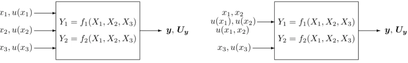
5.6.3 Figure 2 (left) illustrates the (generalized) law of propagation of uncertainty for a measure-ment model with N = 3 mutually independent input quantities X = (X1, X2, X3)> andm= 2

output quantitiesY = (Y1, Y2)>. X is estimated byx= (x1, x2, x3)> with associated standard

uncertaintiesu(x1),u(x2) and u(x3). Y is estimated byy= (y1, y2)> with associated covariance matrix Uy.

Figure 2 (right) applies whenX1 andX2are mutually dependent with covarianceu(x1, x2) associated with the

estimatesx1and x2.

x1, u(x1) -x2, u(x2) -x3, u(x3)

-Y1=f1(X1, X2, X3)

Y2=f2(X1, X2, X3)

- y,Uy

x1, x2

u(x1), u(x2)

u(x1, x2)

-x3, u(x3)

-Y1=f1(X1, X2, X3)

Y2=f2(X1, X2, X3)

- y,Uy

Figure 2 — Generalized law of propagation of uncertainty forN = 3 mutually independent input quantities X1,X2 and X3, andm= 2 (almost invariably) mutually dependent output quantities, and

(right) as left, but for mutually dependent X1 andX2 (5.6.3)

5.6.4 In MCM, a discrete representation of the (joint) probability distribution forX is propagated through the measurement model to obtain a discrete representation of the (joint) probability distribution for Y from which the required summary information is determined.

6 GUM uncertainty framework

6.1 General

6.1.1 The propagation of uncertainty for measurement models that are more general than the form Y =f(X) in the GUM is described (see 6.2 and 6.3). Although such measurement models are not directly considered in the GUM, the same underlying principles may be used to propagate estimates of the input quantities and the uncertainties associated with the estimates through the measurement model to obtain estimates of the output quantities and the associated uncertainties. Mathematical expressions for the evaluation of uncertainty are stated using matrix-vector notation, rather than the subscripted summations given in the GUM, because generally such expressions are more compact and more naturally implemented within modern software packages and computer languages.

6.1.2 For the application of the law of propagation of uncertainty, the same information concerning the input quantities as for the univariate measurement model treated in the GUM is used:

a) an estimatex= (x1, . . . , xN)> of the input quantityX;

b) the covariance matrixUxassociated withxcontaining the covariancesu(xi, xj),i= 1, . . . , N,j= 1, . . . , N,

associated with xi andxj.

6.1.3 The description of the propagation of uncertainty given in 6.2 and 6.3 is for real measurement models, including complex measurement models that are expressed in terms of real quantities. A treatment for complex measurement models is given in 6.4. Also see 5.1.3.

(23)

6.2 Propagation of uncertainty for explicit multivariate measurement models

6.2.1 General

6.2.1.1 An explicit multivariate measurement model specifies a relationship between an output quantityY = (Y1, . . . , Ym)> and an input quantityX = (X1, . . . , XN)>, and takes the form

Y =f(X), f = (f1, . . . , fm)>,

wheref denotes the multivariate measurement function.

NOTE Any particular function fj(X) may depend only on a subset of X, with each Xi appearing in at least one

function.

6.2.1.2 Given an estimatexofX, an estimate ofY is

y=f(x).

6.2.1.3 The covariance matrix of dimension m×massociated withy is

Uy=



 

u(y1, y1) · · · u(y1, ym)

..

. . .. ... u(ym, y1) · · · u(ym, ym)



 ,

where cov(yj, yj) =u2(yj), and is given by

Uy=CxUxC>x, (3)

whereCx is the sensitivity matrix of dimensionm×N given by evaluating

CX =

      ∂f1 ∂X1

· · · ∂f1 ∂XN

..

. . .. ... ∂fm

∂X1

· · · ∂fm ∂XN      

atX =x[19, page 29].

6.2.2 Examples

EXAMPLE 1 Resistance and reactance of a circuit element[JCGM 100:2008 H.2]

The resistanceR and reactanceX of a circuit element are determined by measuring the amplitudeV of a sinusoidal alternating potential difference applied to it, the amplitudeIof the alternating current passed through it, and the phase angleφbetween the two. The bivariate measurement model forRandX in terms ofV,I andφis

R=f1(V, I, φ) =V

I cosφ, X =f2(V, I, φ) = V

I sinφ. (4)

In terms of the general notation,N= 3,m= 2,X≡(V, I, φ)>andY ≡(R, X)>. An estimate y ≡ (R,b Xb)

>

of resistance and reactance is obtained by evaluating expressions (4) at an estimatex≡(V ,b I,bφb)

>

of the input quantityX.

The covariance matrix Uy of dimension 2×2 associated with y is given by formula (3), where Cx is the sensitivity

matrix of dimension 2×3 given by evaluating

     ∂f1 ∂V ∂f1 ∂I ∂f1 ∂φ ∂f2 ∂V ∂f2 ∂I ∂f2 ∂φ      =     cosφ I −

V cosφ I2 −

Vsinφ I sinφ

I −

V sinφ I2

Vcosφ I

   

(24)

atX=x, andUxis the covariance matrix of dimension 3×3 associated withx.

NOTE In the GUM, reactance is denoted byX, which is the notation used here. The reactanceX, a component of the vector output quantity Y, is not to be confused withX, the vector input quantity.

EXAMPLE 2 Reflection coefficient measured by a microwave reflectometer (approach 1)

The (complex) reflection coefficientΓ measured by a calibrated microwave reflectometer, such as an automatic network analyser, is given by the complex measurement model

Γ = aW+b

cW + 1, (5)

where W is the (complex) uncorrected reflection coefficient anda,bandcare (complex) calibration coefficients char-acterizing the reflectometer [10, 16, 26].

In terms of the general notation, and working with real and imaginary parts of the quantities involved, N= 8,m= 2,

X ≡(aR, aI, bR, bI, cR, cI, WR, WI)

>

andY ≡(ΓR,ΓI)

>

. An estimate y ≡ (ΓbR,ΓbI)

>

of the (complex) reflection coefficient is given by the real and imaginary parts of the right-hand side of expression (5) evaluated at the estimatexof the input quantityX.

The covariance matrix Uy of dimension 2×2 associated with y is given by formula (3), where Cx is the sensitivity

matrix of dimension 2×8 given by evaluating

    

∂ΓR ∂a_R

∂ΓR ∂a_I

∂ΓR ∂b_R

∂ΓR ∂b_I

∂ΓR ∂c_R

∂ΓR ∂c_I

∂ΓR ∂W_R

∂ΓR ∂W_I ∂ΓI

∂a_R ∂ΓI ∂a_I

∂ΓI ∂b_R

∂ΓI ∂b_I

∂ΓI ∂c_R

∂ΓI ∂c_I

∂ΓI ∂W_R

∂ΓI ∂W_I     

atX=x, andUxis the covariance matrix of dimension 8×8 associated withx.

EXAMPLE 3 Calibration of mass standards

This example constitutes an instance of a multistage model (see 3.12, 5.4.2 and 5.4.3).

A set of q mass standards of unknown mass valuesm= (m1, . . . , mq)> is calibrated by comparison with a reference

kilogram, using a mass comparator, a sensitivity weight for determining the comparator sensitivity, and a number of ancillary instruments such as a thermometer, a barometer and a hygrometer for determining the correction due to air buoyancy. The reference kilogram and the sensitivity weight have masses mR and mS, respectively. The calibration is carried out by performing, according to a suitable measurement procedure, a sufficient number k of comparisons between groups of standards, yielding apparent, namely, in-air differences δ= (δ1, . . . , δk)

>

. Corresponding buoyancy corrections b= (b1, . . . , bk)

>

are calculated. In-vacuo mass differencesXare obtained from the sub-modelX=f(W), whereW = mR, mS, δ>, b>

>

. An estimatey≡(mb1, . . . ,mbq)

>

of the massesmis typically given by the least-squares solution of the over-determined system of equationsAm=X, whereAis a matrix of dimensionk×qwith elements equal to +1,−1 or zero, according to the mass standards involved in each comparison, and respecting the uncertainties associated with the estimate x

ofX. With this choice, the estimateyis given by

y=UyA

> Ux

−1

x, (6)

where the covariance matrixUy of dimension q×q associated withy is given by Uy = A>Ux−1A

−1

. Ux is the

covariance matrix of dimension k×k associated with x. A more detailed description of the sub-model, as well as a procedure for obtaining Uxin terms ofUw, the covariance matrix associated with the estimatewof W, is available

[3].

The multivariate measurement model for this example can be expressed as

Y =UyA

> Ux

−1

X,

where the measurement function is UyA>Ux−1X. In terms of the general notation,N=k,m=qandY ≡m.

NOTE It is preferable computationally to obtain the estimate given by formula (6) by an algorithm based on orthogonal factorization [13], rather than use this explicit formula.

(25)

6.3 Propagation of uncertainty for implicit multivariate measurement models

6.3.1 General

6.3.1.1 An implicit multivariate measurement model specifies a relationship between an output quantityY = (Y1, . . . , Ym)> and an input quantityX = (X1, . . . , XN)>, and takes the form

h(Y,X) =0, h= (h1, . . . , hm)>.

6.3.1.2 Given an estimatexofX, an estimatey ofY is given by the solution of the system of equations

h(y,x) =0. (7)

NOTE The system of equations (7) has generally to be solved numerically fory, using, for example, Newton’s method [12] or a variant of that method, starting from an approximationy(0) _{to the solution.}

6.3.1.3 The covariance matrix Uy of dimension m×m associated with y is evaluated from the system of

equations

CyUyC>y=CxUxC>x, (8)

whereCyis the sensitivity matrix of dimensionm×mcontaining the partial derivatives∂h`/∂Yj,`= 1, . . . , m,

j= 1, . . . , m, andCxis the sensitivity matrix of dimensionm×N containing the partial derivatives∂h`/∂Xi,

`= 1, . . . , m,i= 1, . . . , N, all derivatives being evaluated atX =xandY =y.

NOTE 1 The covariance matrixUy in expression (8) is not defined ifCy is singular.

NOTE 2 Expression (8) is obtained in a similar way as expression (3), with the use of the implicit function theorem.

6.3.1.4 Formally, the covariance matricesUxand Uy are related by

Uy=CUxC>, (9)

where

C=C−y1Cx, (10)

a matrix of sensitivity coefficients of dimensionm×N.

6.3.1.5 Annex B contains a procedure for formingUy. It is not recommended that Uy is obtained directly

by evaluating expression (10) and then expression (9); such a procedure is less stable numerically.

6.3.2 Examples

EXAMPLE 1 Set of pressures generated by a pressure balance

The pressurepgenerated by a pressure balance is defined implicitly by the equation p= mw(1−ρa/ρw)g`

A0(1 +λp) (1 +αδθ)

, (11)

where mw is the total applied mass,ρa andρw are, respectively, the densities of air and the applied masses,g` is the

local acceleration due to gravity,A0is the effective cross-sectional area of the balance at zero pressure,λis the distortion coefficient of the piston-cylinder assembly,αis the coefficient of thermal expansion, andδθis the deviation from a 20◦C reference Celsius temperature [17].

Let p1, . . . , pq denote the generated pressures for, respectively, applied masses mw,1, . . . , mw,q and temperature

(26)

In terms of the general notation, N = 6 + 2q, m = q, X ≡ (A0, λ, α,δθ1, mw,1, . . . ,δθq, mw,q, ρa, ρw, g`)>

andY ≡(p1, . . . , pq)>.

X andY are related by the measurement model

hj(Y,X) =A0pj(1 +λpj) (1 +αδθj)−mw,j(1−ρa/ρw)g`= 0, j= 1, . . . , q. (12)

An estimatepbj ofpjis obtained by solving an equation of the form (12) given estimates ofA0,λ,α,δθj,mw,j,ρa,ρw

and g`. However, the resulting estimates have associated covariances because they all depend on the measured

quantitiesA0,λ,α,ρa,ρwandg`.

The covariance matrixUyof dimensionq×qassociated withy≡(pb1, . . . ,pbq) >

is evaluated from expression (8), whereCy

is the sensitivity matrix of dimensionq×qcontaining the partial derivatives∂h`/∂Yj,`= 1, . . . , q,j= 1, . . . , q, andCx

is the matrix of dimensionq×(6 + 2q) containing the partial derivatives∂h`/∂Xi,`= 1, . . . , q,i= 1, . . . ,6 + 2q, both

evaluated atX=xandY =y, andUxis the covariance matrix of dimension (6 + 2q)×(6 + 2q) associated withx.

NOTE 1 A measurement function [givingYj (≡pj) explicitly as a function of X] can be determined in this case as

the solution of a quadratic equation. Such a form is not necessarily numerically stable. Moreover, measurement models involving additional, higher-order powers of pare sometimes used [9]. Determination of an explicit expression is not generally possible in such a case.

NOTE 2 There is more than one way to express the measurement model (12). For instance, in place of the form (12), the model based on equating to zero the difference between the left- and right-hand sides of model (11) could be used. The efficiency and stability of the numerical solution of the measurement model depends on the choice made.

NOTE 3 More complete models of the pressure generated by a pressure balance can also be considered [17], which include, for example, a correction to account for surface tension effects.

NOTE 4 Not all the input quantities appear in each equation, with the jth equation involving onlyA0,λ,α,δθj,mw,j,ρa,ρwandg`.

EXAMPLE 2 Reflection coefficient measured by a microwave reflectometer (approach 2)

Another approach to example 2 given in 6.2.2 is to relate the input quantity X ≡(aR, aI, bR, bI, cR, cI, WR, WI)

>

and the output quantityY ≡(ΓR,ΓI)

>

using the bivariate measurement model

h1(Y,X) = 0, h2(Y,X) = 0, (13)

whereh1(Y,X) andh2(Y,X) are, respectively, the real and imaginary parts of (cW + 1)Γ−(aW +b).

An advantage of this approach is that the calculation of derivatives and thence sensitivity coefficients is more straight-forward.

An estimatey≡(ΓbR,ΓbI)

>

of the (complex) reflection coefficient is given by settingX=xin equations (13) and solving them numerically.

The covariance matrix Uy of dimension 2×2 associated with y is evaluated from expression (8), where Cy is the

sensitivity matrix of dimension 2×2 containing the partial derivatives ∂h`/∂Yj, ` = 1,2, j = 1,2, and Cx is the

sensitivity matrix of dimension 2×8 containing the partial derivatives ∂h`/∂Xi,`= 1,2,i= 1, . . . ,8, both evaluated

atX=xandY =y, andUxis the covariance matrix of dimension 8×8 associated withx.

EXAMPLE 3 Reflectometer calibration

The calibration of a reflectometer (example 2 of 6.2.2) is typically undertaken by measuring valuesW of the uncorrected reflection coefficient corresponding to a number of standards with reflection coefficients Γ. Often, three standards are used, giving the three (complex) simultaneous equations

(cWj+ 1)Γj−(aWj+b) = 0, (14)

forj= 1,2,3. Separation of these equations into real and imaginary parts gives rise to six simultaneous linear equations that are solved for estimates of the real and imaginary parts of the calibration coefficients a,bandcgiven estimates of the real and imaginary parts of the uncorrected reflection coefficientsWjand of the reflection coefficientsΓjfor the

standards.

In terms of the general notation,N= 12,m= 6,X≡(W1,R, W1,I,Γ1,R,Γ1,I, W2,R, W2,I,Γ2,R,Γ2,I, W3,R, W3,I,Γ3,R,Γ3,I)

>

andY ≡(aR, aI, bR, bI, cR, cI)

>

(27)

The input and output quantities are related by a multivariate measurement model, where, forj= 1,2,3,h2j−1(Y,X) andh2j(Y,X) are, respectively, the real and imaginary parts of the left-hand side of expression (14).

An estimatey≡(baR,baI,bbR,bbI,bcR,bcI) >

of the (complex) calibration coefficients is given by using the estimates ofWj

andΓjin equations (14) and solving these equations numerically.

The covariance matrix Uy of dimension 6×6 associated with y is evaluated from expression (8), whereCy is the

sensitivity matrix of dimension 6×6 containing the partial derivatives ∂h`/∂Yj,`= 1, . . . ,6,j= 1, . . . ,6, andCx is

the sensitivity matrix of dimension 6×12 containing the partial derivatives∂h`/∂Xi,`= 1, . . . ,6,i= 1, . . . ,12, both

evaluated atX=xandY =y, andUxis the covariance matrix of dimension 12×12 associated withx.

NOTE 1 If a computer system capable of operating with complex quantities is available, separation of these equations into real and imaginary parts is unnecessary. The equations can be solved “directly” fora,bandc.

NOTE 2 Thejth equation involves only the four input quantitiesWj,R,Wj,I,Γj,R andΓj,I.

6.4 Propagation of uncertainty for models involving complex quantities

Annex A covers the algebraically efficient determination of the partial derivatives of first order of complex mul-tivariate measurement functions. These derivatives are needed in a particularization of the law of propagation of uncertainty to such models. The treatment can be extended to complex multivariate measurement models in general.

EXAMPLE Reflection coefficient measured by a microwave reflectometer (approach 3)

Consider again example 2 given in 6.2.2.

The complex output quantityY ≡Γ is related to the complex input quantityX= (X1, . . . ,X4)>≡(a,b,c,W)>by the measurement model (5). Using annex A,Cx, a sensitivity matrix of dimension 2×8, is given by evaluating

CX =

Ca Cb Cc CW

, with

Ct=M

∂Γ ∂t

, t≡a,b,c,W, at the estimatexofX. For instance, since

∂Γ ∂b =

1

cW + 1, (15)

the further use of annex A gives

Cb=

QR −QI QI QR

,

whereQRandQI denote the real and imaginary parts, respectively, of the right-hand side of expression (15). The covariance matrixUy of dimension 2×2 associated withy≡Γb, where

Uy=

u(Γb_R,Γb_R) u(Γb_R,Γb_I)

u(ΓbI,ΓbR) u(ΓbI,ΓbI)

≡

u2(Γb_R) u(Γb_R,Γb_I)

u(ΓbI,ΓbR) u2(ΓbI)

,

is evaluated from expression (A.1) of annex A, whereUxis the covariance matrix of dimension 8×8 associated withx.

6.5 Coverage region for a vector output quantity

6.5.1 General

6.5.1.1 In electrical metrology, for example, it is appropriate to treat a vector output quantity as a single entity and in dealing with summaries of the joint probability distribution for this quantity to maintain as much information as possible.

JCGM 102:2011. October 2011

JCGM 102

:

2011

Evaluation of measurement

data – Supplement 2 to the

“Guide to the expression of

uncertainty in measurement” –

Extension to any number of

output quantities

Évaluation des données de mesure

−

Supplément 2 du “Guide pour

l’expression de l’incertitude de mesure”

– Extension à un nombre quelconque de

grandeurs de sortie

Copyrights

Droits d’auteur

2011

Evaluation of measurement data — Supplement 2

to the “Guide to the expression of uncertainty in

measurement” — Extension to any number of

output quantities

´

Evaluation des donn´

ees de mesure — Suppl´

ement 2 du “Guide pour l’expression

de l’incertitude de mesure” — Extension `

a un nombre quelconque de grandeurs

de sortie

Contents

Annexes

Foreword

Introduction

Evaluation of measurement data — Supplement 2

to the “Guide to the expression of uncertainty in

measurement” — Extension to any number of output

quantities

1

Scope

2

Normative references

3

Terms and definitions

4

Conventions and notation

5

Basic principles

5.1

General

5.2

Main stages of uncertainty evaluation

5.3

Probability density functions for the input quantities

5.4

Propagation of distributions

5.5

Obtaining summary information

5.6

Implementations of the propagation of distributions

6

GUM uncertainty framework

6.1

General

6.2

Propagation of uncertainty for explicit multivariate measurement models

6.3

Propagation of uncertainty for implicit multivariate measurement models

6.4

Propagation of uncertainty for models involving complex quantities

6.5

Coverage region for a vector output quantity