Assembling and Characterizing the Efficiency of an Injection Locked Laser System for Cold Neutral Atom Optical Traps

Assembling and Characterizing the Efficiency of an Injection Locked Laser System for

Cold Neutral Atom Optical Traps

A Senior Project presented to

the Faculty of the Physics Department

California Polytechnic State University, San Luis Obispo

In Partial Fulfillment

of the Requirements for the Degree Bachelor of Science

by

Alexandra Crawford June, 2018

Abstract

i Table of Contents

List of Figures ... ii

List of Tables ... iv

1. Introduction ...1

1.1 Quantum Computing ...1

1.1.1 What are Qubits? ...1

1.1.2 Essentials of Quantum Computers ...1

1.2 Using Cold Neutral Atoms as Qubits ...2

1.3 Overview...3

2. Theory ...4

2.1 Optically Cooling and Trapping Neutral Atoms ...4

2.1.1 Doppler Effect: Cooling Atoms Down ...4

2.1.2 Trapping Atoms in Detuned Laser Light ...5

2.1.3 Utilizing Polarization Dependence to Increase Trap Integrity ...7

2.1.4 Pinhole Diffraction Pattern ...7

2.2 Injection Locked Laser System...9

2.2.1 “Seed” and “Receiving” Laser Relationship ...9

2.2.2 Resonant Cavity Using Laser Diodes ...9

2.2.3 Grating Feedback Loop ...10

2.3 Understanding Certain Resonant Modes of the Seed and Receiving Lasers “Match” to Lock ...10

2.3.1 Gain Medium in a Laser ...10

2.3.2 Homogeneous Broadening ... 11

2.3.3 Inhomogeneous Broadening ...12

2.3.4 “Overlapping” the Resonant Modes of Each Laser to Effectively Lock the System ...12

3. Experiment ...14

3.1 Injection Locked Laser Setup ...14

3.1.1 Collimation of Seed and Receiving Lasers ...14

3.1.2 Tuning Range of Seed Laser ...16

3.1.3 Beam Path Setup ...18

3.1.4 Stabilization of Laser Diode Temperatures ...20

3.1.5 Measuring Injection Lock Efficiency ...25

3.2 Effects of Adjusting Seed Output Power on System Locking Efficiency...27

3.3 Observing Injection Lock Efficiency for Variable Seed Laser Diode (LD) Current ...31

3.4 Effects of Adjusting Seed Laser Temperature on System Locking Efficiency ...33

4. Conclusions ...36

4.1 Experimental Results ...36

4.2 Future Work ...36

References ...38

Appendix ...40

ii List of Figures

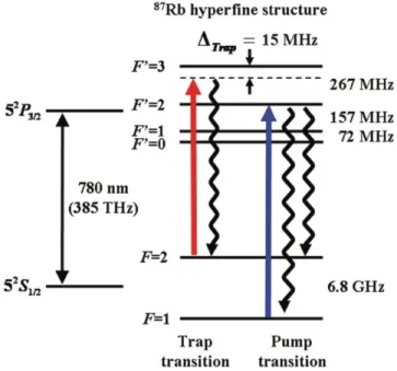
Figure 1: Diagram of Rubidium-87 hyperfine structure where the Doppler cooling process of the trap laser is represented by the red transition. The set of arrows that transition to the S1/2 F=1 level is an undesired transition. The pump laser (represented by dark blue) is the pump laser that corrects this transition, returning it to the S1/2 F=2 level [9]. ... 5 Figure 2: (a) Two-dimensional potential energy well lattice in the x-y plane where incoming lasers create standing waves and the atoms are trapped in either regions of high or low intensity. (b) Trapped atoms in anti-nodes of laser standing waves in positions of high intensity. ... 6 Figure 3: Intensity distribution from diffraction pattern of circular aperture (r = 50µm) [13]. ... 8 Figure 4: Trapping potential energy for two oppositely circularly polarized laser beams through a circular diffraction aperture each at an angle of 0.055 radians [6]. The two beam angles can be adjusted to move trapped atoms into a common trap position. ... 8 Figure 5: Representation of volumes and surfaces used in establishing a diffraction theory [15]. ... 9 Figure 6: Littrow ECDL configuration [19]. ... 10 Figure 7: Gain saturation in a homogeneously broadened laser where the cavity modes are separated by nfsr. (a) When the laser is turned on the gain coefficient has the smallest value so that several modes are above the threshold value gth. (b) The gain coefficient is reduced due to gain saturation when the

irradiance in the cavity modes above threshold grows. This reduces the number of modes above the threshold value. (c) Gain saturation reduces the gain coefficient so that only the mode nearest the line center no reaches the threshold value. This results in a single mode being lased [18]... 12 Figure 8: Comparison of saturation in (a) a homogeneously broadened profile and (b) an

inhomogeneously broadened profile, illustrating “hole burning”, where ao denotes the initial gain curve and as is the saturated gain curve [23]. ... 13 Figure 9: Laser diode pin layout (assuming the output beam is directed into the page) ... 14 Figure 10: Receiving laser diode and lens casing with contents arranged in order. The extra spacer ring that was removed is indicated. ... 15 Figure 11: Beam path diagram created to collimate seed and receiving lasers ... 15 Figure 12: Fine adjustment knobs for the mirror-grating arm on the far left. Illustration of the spread of wavelengths over different angle values [24]. ... 17 Figure 13: (a) Injection locked laser system optical component setup (color online). (b) The beam path polarization propagation where a = 45˚ and b is a variable angle ranging from 0˚ to 45˚ that is

dependent upon the half wave plate rotation. ... 19 Figure 14: Incorrect waveforms of laser temperatures on the Thorlabs Combi Controllers. The

iii

pseudo-stable system with a subtle drift over time can cause complications in maintaining a stable

frequency on the diode laser. (color online) ... 22

Figure 15: Receiving laser temperature oscillating towards and at steady state (color online) ... 24

Figure 16: Seed laser temperature oscillating at steady state ... 25

Figure 17: Injection lock efficiency over different HWP rotation values (power of seed laser). ... 28

Figure 18: Placement of power meters within beam path indicating the measurements taken in tables 29 Figure 19: Power measurements throughout the injection locked laser system for different HWP rotation values. (color online) ... 30

Figure 20: Injection lock efficiency with HWP rotated to 328˚ for 75% of maximum power throughput ... 32

Figure 21: Injection lock efficiency with HWP rotated to 341˚ for maximum power throughput ... 32

Figure 22: Injection lock efficiency for variable laser diode temperature and HWP at 328˚ for 75% of maximum power throughput... 34

iv List of Tables

1 1. Introduction

1.1 Quantum Computing

The conventional approaches to furthering classical computer technology follow the trend of reducing component sizes to increase computing power. However, as component sizes approach atomic scales, quantum effects begin to interfere with their ability to function reliably in a classical manner [1]. For example, electrons used to determine the value of a classical bit (having the value of either 1 or 0) will become compromised if the electron tunnels through boundary material that is only atoms thick, resulting in a loss or corruption of information. By utilizing quantum physics and quantum information science, the size limit that classical systems are approaching can be avoided.

Quantum information science is based in the utilization of quantum mechanical properties to perform computations as well as manipulate and transmit information [1]. The study of the preparation and control of quantum states within physical systems has also led to the theoretical understanding that certain computations and simulations performed by a quantum computer will be done more efficiently compared to a classical system [2]. Quantum systems are able to store and keep track of an exponential amount of complex numbers and perform calculations as the system is scaled up. It has already been theoretically shown that quantum algorithms such as Shor’s factoring algorithm, which runs in polynomial time to find the prime factors of an integer, provide advantages over classical algorithms that take exponential amounts of processing power to compute [1].

1.1.1 What are Qubits?

The bit is an essential and fundamental concept of the classical computation system that is used to construct and store information and can have a value of either 0 or 1. Since quantum computation systems are built on analogous concepts to classical systems, the quantum-bit or “qubit” also has states |0⟩ and |1⟩, as well as a superposition of these two states:

(1) |𝛹⟩_{& ()*+,} = 𝛼 |0⟩ + 𝛽 |1⟩

where α and β are the complex amplitudes for the respective states, and

(2) |𝛼|2 _{+ |𝛽|}2 _{= 1}

is the normalization condition that the function follows [2]. Expressing the qubit as a mathematical object, where the states of the qubit are unit vectors in a two-dimensional complex vector space, the states and are referred to as the computational basis states for the system [4]. However, we cannot determine the state of the qubit by measuring the values of the amplitudes within the superimposed state, since the act of observation will collapse the state of the system to result in one of the two basis states, each with a 50% probability of occurring.

Entangling two qubits in a system results in a superimposed state that cannot be written as a product of the states of two individual qubits. The general state of two qubits,

(3) |𝛹⟩_{2 𝑞𝑢𝑏𝑖𝑡𝑠}= 𝛼|00⟩ + 𝛽|01⟩ + 𝛾|10⟩ + 𝛿|11⟩

is a four-dimensional vector where α, β, γ, and δ are the complex amplitudes for each respective distinguishable state of the system with |𝛼|2 _{+ |𝛽|}2 _{+ |𝛾|}2 _{+ |𝛿|}2 _{= 1.}

1.1.2 Essentials of Quantum Computers

2

Regardless of the system used to physically create a quantum computer, there are five requirements for the implementation of quantum computing [3]:

1. A scalable physical system with well characterized qubits

A quantum computer needs a system containing a collection of physical embodiments of qubits, such as a simple quantum two-level system. The energy states of an electron within an atom, utilizing the atom’s two ground states, are used as the and states of the qubit

respectively. The permitted states of a single qubit fill up a two-dimensional complex vector space, allowing the general superimposed state to assume infinite values. The general state of two qubits is a four-dimensional vector, one dimension for each of the four basis states of the combined 2-qubit system.

2. The ability to initialize the state of the qubits to a known state

A technical requirement for any computing system is the ability to initialize registers to a known value before starting a computation.

3. Relevant coherence time that is much longer than the gate operation time

Coherence times are associated with the interaction of a qubit with its environment and neighboring qubits. Having a sufficiently long coherence time, relevant to its function as a qubit and longer than the gate operation time, ensures the integrity of the computation.

4. A “universal” set of basic quantum gates

The classical equivalent to performing computations in a quantum computer is the incorporation of a “universal” system of quantum gates to perform a sequence of unitary transformations on the system of qubits. “Universal” quantum gates refer to any set of gates utilized in a quantum computer which can be reduced to a sequence of basic finite operations. Essentially, any algorithm can be made by a series of these basic gates.

5. A qubit-specific measurement capability

The final requirement of a quantum computer is the ability to read out the computation result, specifically the ability to measure specific qubits.

1.2 Using Cold Neutral Atoms as Qubits

Introducing an optical lattice system as a neutral atom (qubit) trap, holds good prospects for satisfying several of the requirements of quantum computers. An appealing feature of using neutral atoms as qubits is how their electronic ground state couples extremely weakly to the environment or neighboring atoms, allowing for long coherence times and tight atomic confinement in the physical realization of memory registers. The ability to induce inter-atomic coupling (entanglement) can be implemented through dipole-dipole interactions, ground state collisions, or photon exchange [4]. Initialization and readout of states can be done with techniques in the long-established field of laser spectroscopy [5]. The method utilized in this experiment to initialize the state of a qubit is through the absorption and spontaneous emission of a photon. “The weak atomic interactions also make it

relatively straightforward to trap and cool neutrals in large numbers, with favorable implications for scaling to many qubits” [4].

3

for trapping an atom (qubit) to reduce the rate of photon scattering, where the probability of a photon exciting the trapped atom is lowered the further the laser is detuned from resonance. At the same time, increasing the intensity of the trap laser maintains a strong trapping potential for the atom [4], which is the motivation for implementing an injection locked laser into the system. Implementing an injection locked laser system allows the power input to the seed laser diode to be reduced while still providing a high intensity beam to the system via the receiving laser diode. The large intensity output beam

directed into the atom cloud allows the atom to remain within a large trap potential.

1.3 Overview

Section 2 reviews the theory behind the experimental setup: introducing the cooling of atoms and the effects line shape broadening has on locking efficiency, while focusing on the injection locked laser system and the optical trapping of atoms in a pinhole diffraction pattern with detuned laser light. Section 3 provides details on the experimental setup such as the components of the injection locked laser system, the detuning of the seed laser frequency, and the output beam path setup. The

4 2. Theory

2.1 Optically Cooling and Trapping Neutral Atoms

As stated earlier, qubit states within this experiment are physically realized through the two hyperfine ground states of cold neutral Rubidium-87 atoms, for their long coherence times and weak coupling to their surrounding environment. Placing these atoms in an Ultra-High Vacuum (UHV) setting to minimize the perturbations by other gases allows for more effective cooling using a Magneto-Optical Trap (MOT). Atoms are collected in the center of the trap with a quadrupole magnetic field generated by two Anti-Helmholtz coils due to the center of the magnetic field gradient being zero. The combination of cooling these atoms within a MOT, through Zeeman Effect and Doppler Cooling techniques, will bring the atom cloud temperature to approximately 200 µK [7], which is cold enough (moving slowly enough) to incorporate optical dipole traps.

Optical dipole traps are structures of far-detuned laser light in either the so-called red or blue directions, that rely on the interaction between the laser’s electric field and the trapped atom to be effective. Red detuning a laser in a trapping system requires the laser frequency (and therefore its energy) to be less than the resonance frequency of the trapped atom. A blue detuned laser in comparison is above the resonance frequency of the atom, with a higher associated energy. Blue detuned (BDT) traps have the advantage above red detuned (RDT) traps in that they lower the

probability of the atom being excited by a stray photon because it resides in dark spots, helping provide longer coherence times to maintain the state of an (entangled) atom for the integrity of the calculation.

2.1.1 Doppler Effect: Cooling Atoms Down

Doppler cooling utilizes RDT laser beams propagating in both directions along a single axis to reduce the velocity of atoms within an atomic cloud regardless of the direction of travel. Experimentally, the atomic cloud will be localized in the center of the MOT and cooled using three pairs of RDT beams, one for each Cartesian axis. Localization of the atoms is due to the gradient of the quadrupole magnetic field and the Zeeman effect, while the slowing of atoms is due to the Doppler effect. The amount of detuning below the resonant frequency of the atom is dependent upon the MOT magnetic field gradient and provides a velocity dependence on the radiation pressure opposite the direction of the atom’s propagation. Experimentally, our lasers were determined to utilize a 10 MHz (or 1.5 linewidths) red shift from atomic resonance based on the specific magnetic field gradient measured within our MOT.

Atoms are cooled through the transfer of momentum of the photon absorption and emission processes that occur in the laser beam path near atomic resonance. The atom’s velocity is slowed through cycles of near-resonant absorption of a photon, where the carried momentum

(4) 𝑝_; = ħ𝑘 = 2𝜋ħ_?

5

atom back into a higher energy level if it goes into the wrong ground state. Figure 1 illustrates this concept.

Figure 1: Diagram of Rubidium-87 hyperfine structure where the Doppler cooling process of the trap laser is represented by the red transition. The set of arrows that transition to the S1/2 F=1 level is an undesired transition. The pump laser (represented by dark blue) is the pump laser that corrects this transition, returning it to the S1/2 F=2 level [9].

2.1.2 Trapping Atoms in Detuned Laser Light

BDT traps utilize trapping lasers that have higher frequencies (and energies) than the resonance frequency of the atom, so that the atom will not be stimulated into a higher energy level from the photons of the trapping laser. Both RDT and BDT optical dipole traps rely on the induced dipole moment in the trapped atom by the electric field of the lasers. If the frequency of the electric field’s change in orientation is slow compared to the frequency at atomic resonance, the orientation of the induced dipole moment will change to align parallel to the field, resulting in the atom being attracted to positions of high field intensities. Below atomic resonance, the dipole potential energy

(5) 𝑈 = −𝑝⃗ ⋅ 𝐸E⃗

6

RDT optical dipole traps usually use large detunings and high intensities to keep scattering rates as low as possible at certain potential energy depths [8]. To maintain a deep potential energy well for the atom to reside in, the detuning needs to be small which means the frequency of the laser trap is close to the resonance frequency of the atom. This presents the problem of stimulating the trapped atom into an excited state by a stray photon from the trap. Especially in a RDT trap, where the atom is trapped in regions of high intensity, the probability of this occurrence is high. To avoid using detuned frequencies that are too close to the atom’s resonance frequency, larger detunings are used with the trade-off of higher laser intensities to maintain the shape of the potential energy well. As the frequency of the detuned laser moves farther from the resonant frequency of the atom, the sides of the potential energy well lower, rendering the trap less effective the farther the laser is detuned [11]. The detuning in the blue direction is bound in the high energy direction by the ionization energy of the atom [8] and bound at the low end by the atom’s resonant frequency. Blue detuned traps avoid the trade-off of needing higher intensity lasers for a larger detuning through the nature of how they trap atoms in positions of lowest intensity, reducing the interaction between the laser and the atom further than far RDT traps [10].

To confine an atom in two dimensions a potential energy pattern can be created through potential energy wells in two perpendicular directions (figure 2a) using either red or blue detuned laser light. Since a laser beam has a Gaussian intensity distribution in the radial

direction and a Lorentzian axial distribution, a single potential energy well can confine an atom in all three spatial dimensions for a RDT trap. Confining several atoms in three dimensions in a RDT system can be achieved through a standing wave from a single laser beam (figure 2b). Here the atoms, attracted to positions of highest intensity, are confined in the x, y, and z

directions by lower intensity regions within the interference pattern and outside the beam. Upon initial inspection, one could argue this trapping pattern cannot be used for a BDT system

because the atom, attracted to positions of low intensity, will only be confined in the axial direction and not in the radial dimension. However, a “Nested Gaussian” standing wave pattern was conceived and computationally analyzed by Travis Frazer in his senior project to trap Rubidium-87 atoms in a 1D lattice of BDT dipole traps [12].

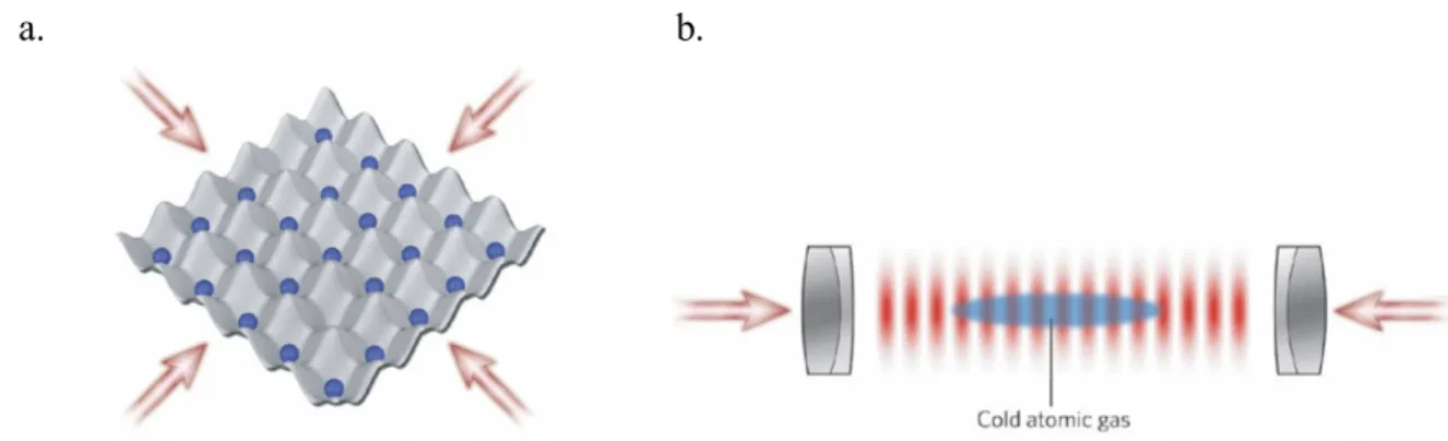
a. b.

Figure 2: (a) Two-dimensional potential energy well lattice in the x-y plane where incoming lasers create standing waves and the atoms are trapped in either regions of high or low

intensity. (b) Trapped atoms in anti-nodes of laser standing waves in positions of high intensity.

7

profile, displacements of the atom from the center of the beam waist (potential energy trap) will return it to the center which contains the region of highest intensity. However, this is a RDT trap that does not have confinement in the axial direction, so there is a probability that the trapped atom can escape the potential energy well through the lowered limits along the axis [8]. Optical lattices may also trap atoms in a periodic structure of bright and dark spots in up to three dimensions. A 3D optical lattice could contain a large concentration of individually trapped atoms with separations of half the wavelength of the trapping laser. The challenge that arises with this structural configuration is the addressing of individual atoms while maintaining the integrity of the other atom’s states. A pinhole diffraction pattern can be utilized to create a 2D array of light and dark spots that can be used in either red or blue detuned systems, which is utilized within this experimental setup. An advantage of creating pockets of light or dark spots for trapping individual atoms is the reduced probability of the atom escaping from the potential energy well trap due to the higher well walls. The 2D array utilized in this experiment also allows each atom to be individually addressed while maintaining the coherency of the system.

2.1.3 Utilizing Polarization Dependence to Increase Trap Integrity

Atoms can be confined in “mobile” traps that allow for entanglement for quantum computations. Since dark traps are surrounded by higher intensity regions, maintaining the atom in a trap while another trap is brought to that same position poses the issue that bright regions will repel the atom. However, two opposite circularly polarized beams entering a single diffraction aperture (or aperture grid) can confine atoms with different magnetic quantum number (mF) values so that they remain in their respective dark traps while the traps converge. Since the different mF values of the atoms interact with their respectively polarized beam, the light regions of the second trap will not affect it as strongly, allowing the traps to converge [6].

2.1.4 Pinhole Diffraction Pattern

8

Figure 3: Intensity distribution from diffraction pattern of circular aperture (r = 50µm) [13].

Figure 4: Trapping potential energy for two oppositely circularly polarized laser beams through a circular diffraction aperture each at an angle of 0.055 radians [6]. The two beam angles can be adjusted to move trapped atoms into a common trap position.

For the experimental setup described within this paper, the diffraction pattern regimes utilized are the Rayleigh-Sommerfeld (RS) and Hertz-vector diffraction regions. The RS regime is also known as a “scalar diffraction region” because the resultant pattern can be calculated simply using the sign and size of the electric field rather than its full vector nature. Theoretical modeling begins with the consideration of the situation depicted in figure 5, where

9

Figure 5: Representation of volumes and surfaces used in establishing a diffraction theory [15].

In the scalar diffraction theory of light, the RS diffraction formula for a circular aperture [16] is (6) 𝑉_G+H(0,0, 𝑧) = 𝐴 ∬_OP& _RQS× (1 − 𝑖𝑘𝑅V)

WXY (+ZRS)

RS[ 𝑅′𝑑𝑅′𝑑𝑓′

along an optical axis +z and where 𝑅′ = _ 𝑥′2 _{+ 𝑦′}2 _{+ 𝑧}2_{. This utilizes the simultaneous}

assumption that the radius of S1 approaches zero and the Sommerfield radiation condition is applied, where the radiation across the surface S2 is composed of only outward waves and the distance from P1 to the surface S2 becomes very large [14]. The RS regime is applicable for distances along the optical axis that are much greater than the wavelength of light used [16]. For distances smaller than those used by RS, noted by the Hertz-vector diffraction theory (HVDT), the entire vector expression of the electric and magnetic fields of light are needed to calculate the diffraction pattern extremely close behind the aperture [17].

2.2 Injection Locked Laser System

Lasers emit both spatially and temporally coherent light through optical amplification based on both stimulated emission and population inversion. The total emitted light of the laser is produced through a combination of spontaneous and stimulated emission, but the rate of stimulated emission within the gain medium must be much greater due to the coherence requirement as well as the intended direction of the emitted photons. This contributes to the uniform directionality of the output beam. Spatial coherence refers to the low divergence rate of the laser beam and its ability to be collimated over long distances. Temporal coherence implies that a single frequency of polarized light has a matched phase and amplitude along the beam [18].

Injection locked laser systems utilize continuous wave (CW) lasers specifically to provide a tunable frequency light source with a higher power output than the seed laser alone is able to provide. In this system, one laser’s output beam is directed into the cavity of a second laser. To distinguish between the two lasers, we will name the laser whose output beam is directed into the cavity of another as the seed laser, and the receiving laser will be the laser whose cavity is flooded with the light of the first. Within this experiment, the optical injection locking system is used as an amplification process to create a detuned light source for trapping individual Rubidium atoms within the MOT via a pinhole diffraction pattern.

2.2.1 “Seed” and “Receiving” Laser Relationship

In the injection locked system, the seed laser is tuned to produce a desired wavelength of light that is near the natural wavelength produced by the laser. We specifically use 120-mW, 785-nm diodes (SONY LD TO18, 5.6-mm diode package) within all lasers in our experimental setup, each producing a natural wavelength of approximately 784 nm which is within the near-infrared (NIR) frequencies. Our seed laser is tuned to output 780 nm using a diffraction grating, which is then optically isolated and directed into the cavity of the receiving laser. The inputted light will flood the receiving laser’s cavity to produce the seed laser’s tuned wavelength as opposed to the natural wavelength of the receiving laser.

2.2.2 Resonant Cavity Using Laser Diodes

10

[18]. Here the amount of stimulated emission due to photons passing through is larger than the amount of photon absorption. An effective optical resonator cavity is an essential component of a laser, surrounding the gain medium where population inversion occurs. Light confined within a cavity with highly reflective mirrors, reflects multiple times to produce standing waves for certain resonance frequencies. The resonant frequencies produced are dependent upon the length of the cavity

(7) 𝛥𝜈 = G

Od

and can be adjusted as the length of the cavity is altered [8].

The seed laser within our experimental setup consists of two resonant cavities: the laser diode cavity and an external cavity that utilizes an Edmund Optics J43-775 diffraction grating with 1800 lines/mm. This makes the seed laser an External Cavity Diode Laser (ECDL)

utilizing a Littrow configuration (figure 6) to change the beam’s longitudinal modes, which are standing waves along the optical axis of the laser. The external cavity is now the dominating mechanism, changing the standing wave’s longitudinal modes due to the new cavity length and amplifying a single output mode with a narrow line width.

Figure 6: Littrow ECDL configuration [19].

2.2.3 Grating Feedback Loop

In order to reduce the lasing bandwidth and stabilize the output beam frequency, a grating feedback loop is incorporated into the seed laser’s external resonant cavity. The reference frequency in this experiment is stabilized using a dichroic-atomic-vapor laser lock (DAVLL), where a linearly polarized beam passes through a Rubidium vapor filled Fabry-Perot (FP). The tuned frequency that the seed laser is outputting is compared to the frequency from the FP. Deviations of the seed laser frequency is corrected using a piezoelectric transducer (PZT) to adjust the angle of the diffraction grating (which in turn adjusts the tuning of the seed laser frequency) [19]. More detail on the DAVLL and the electronics used can be found in reference 19.

2.3 Understanding Certain Resonant Modes of the Seed and Receiving Lasers “Match” to Lock

11

Many of the general principles that are presented in Pedrotti [14] for gas lasers, also hold true for diode lasers. When describing gain media within a laser, Helium-Neon (HeNe) lasers utilize the energy states of valence electrons within the gaseous mixture of the lasing cavity while diode lasers utilize a p-n junction. The laser diode used in this experiment is a double heterostructure, where stimulated emission occurs within a thin active layer of material

surrounded by p-doped and n-doped layers. Heterojunctions within semiconductor laser diodes are used to simultaneously confine photons and carrier electrons within that region during lasing [20]. However, we can still describe the gain media through the gain coefficient

(8) 𝛾 = 𝐼_fQfg

where Ninv is the population inversion that exists in steady state: (9) 𝛾 = 𝜎𝑁_+jk = 𝜎(𝑁_O− 𝑁_&) = 𝜎(𝑁_G− 𝑁_k)

For the semiconductor diode laser, N2 can be replaced by Nc (the excess above the thermal equilibrium concentration of electrons in the conduction band) and N1 can be replaced by Nv (the excess of electrons in the valence band) [21].

Optical amplification in the gain medium of a laser occurs through stimulated emission, where transitions of electrons from an excited state to a lower energy state are induced. In a four-level system, a lower threshold pump power can be achieved where the lower lasing level is above the ground state, allowing for depopulation to occur spontaneously. The unexcited gain medium would then exhibit strong absorption to achieve population inversion and thus a net gain within the cavity. If, the lower energy level would not accumulate a significant population density while lasing, this would ensure that the produced lase radiation is not reabsorbed. However, the electrons would then not be able to repeat the lasing cycle.

For the ideal four level case, the gain coefficient is simplified to

(10) 𝛾 = ;l

&mg/go

where the small signal gain coefficient is γo and the saturation irradiance is Is. Generally, the gain coefficient is smaller for larger irradiance due to gain saturation, which occurs because induced stimulated emission events reduce the steady state population of the upper lasing level [18].

2.3.2 Homogeneous Broadening

Broadening in laser physics affects the spectroscopic line shape of the laser’s emission profile, which is due to the excitement and following relaxation of the atomic electron between an excited state and ground state. Since the energy difference between these states is equal to the emitted photon’s energy, and thus proportional to its frequency, the fluctuations in photon energy will result in a range of output laser frequencies. On a spectrometer, a broadened spectroscopic profile will be seen as opposed to the narrow peak of a theoretically ideal single frequency emitting laser [18].

Homogeneous broadening refers to the uniformity of broadening type for each quantum emitter in a system. The line shape factor g(ν') determines the strength of the interaction of an atomic system with an incident field of frequency ν', while homogeneous broadening

mechanisms broaden the line width Δν of the frequency response of each atom similarly [18]. The broadening mechanism that predominantly affects this experimental setup is lifetime broadening, whose effects lead to a Lorentzian line shape function

(11) 𝑔(𝜐) = rst

OP[(svsl)[m(rst/O)[]

12

(12) Δ𝜈_y = &

OPz & {[+

&

{|+ 2𝑟G~•€

where τ1 and τ2 are the lifetimes of the lower and upper levels within the transition respectively. The τ terms are the contributions from the lifetime broadening process while the rate of

collisions term rcol is the pressure broadening contribution [14], which is negligible in our experimental setup.

2.3.3 Inhomogeneous Broadening

In general, both homogeneous and inhomogeneous broadening occur within the same gain system. Inhomogeneous broadening refers to the combination of homogeneous gain bandwidth results and environmental factors that cause the center frequencies of each atom in an assembly to differ, producing a Gaussian line shape function [18]. In semiconductor diodes, the Gaussian profile is not always a good approximation for the more complicated Fermi-Dirac distribution that is applied to the semiconductor laser [21]. The gain medium in an

inhomogenously broadened medium has contributions from groups of atoms with different center frequencies and relatively narrow homogenous bandwidths. As a result, the growing irradiance reduces the population inversion so that the laser output can consist of frequencies corresponding to several different cavity modes [18]. Depletion occurs in a band centered on the oscillation frequencies (modes) and is called “hole burning”. The shape of the hole is an

inverted Lorentz profile with a width () equal to the inverse of the radiative lifetime of the lasing transition [22]. If the radiative width of the laser transition is smaller than the width of the gain curve, then inhomogeneous broadening is observed. Since the lasers used in this experiment are semiconductor diodes, Doppler broadening (which only applies to a gas medium) is not considered in this system.

2.3.4 “Overlapping” the Resonant Modes of Each Laser to Effectively Lock the System

In a homogeneously broadened laser, the gain envelope contains several resonant modes of the lasing cavity. As the growing irradiance reduces the population inversion so that the gain coefficient is lowered, the number of modes above the threshold value approaches one. As shown in figure 7, this is due to the uniform broadening across the curve, resulting in a single mode laser [18]. Changes in temperature of the laser system will shift the gain curve, which results in a shift in lasing frequency. On the spectrometer, this can be seen with mode hopping of the central lasing frequency.

13

that several modes are above the threshold value gth. (b) The gain coefficient is reduced due to gain saturation when the irradiance in the cavity modes above threshold grows. This reduces the number of modes above the threshold value. (c) Gain saturation reduces the gain coefficient so that only the mode nearest the line center no reaches the threshold value. This results in a single mode being lased [18].

In an inhomogeneously broadened laser, reduction of the gain coefficient is seen at the resonant modes of the cavity, resulting in “hole burning” of the gain curve. Figure 8 compares the saturation of a homogeneously and inhomogeneously broadened profile.

Figure 8: Comparison of saturation in (a) a homogeneously broadened profile and (b) an inhomogeneously broadened profile, illustrating “hole burning”, where ao denotes the initial gain curve and as is the saturated gain curve [23].

14 3. Experiment

3.1 Injection Locked Laser Setup

This experiment implements an injection locking system to two continuous wave (CW) Gallium Aluminum Arsenide (GaAlAs) diode lasers operating in the NIR, specifically utilizing wavelengths of 780 nm and 784 nm for the seed and receiving lasers respectively. Responsibilities of this project include replacing the laser diodes in each laser, collimating both of the laser beams, lowering the threshold current to increase the tuning range of the seed laser, setting up and aligning the table optics to achieve injection locking, stabilizing the temperatures on both thermoelectric cooler (TEC)

controllers, characterizing the system lock efficiency as a function of seed laser power, characterizing the system lock efficiency for varying current supplied to the seed laser diode, and characterizing the system lock efficiency as a function of the seed laser temperature. Some challenges were faced during the alignment of the injection locking of the laser system and during the stabilization of the laser temperatures. The following sections will discuss the procedures of these processes as well as solutions to the experimental challenges mentioned above.

3.1.1 Collimation of Seed and Receiving Lasers

The NIR frequency diodes within both the seed and receiving lasers needed to be installed first. A diagram of the pin layout on each of the laser diodes is shown in figure 9, where their orientation correlates to a diode that is facing into the page and rotated so that the output beam is vertically polarized.

Figure 9: Laser diode pin layout (assuming the output beam is directed into the page)

Each laser needed to be collimated to an infinite focal point, so that each beam can be considered to not have a significant beam spread within the system. Both lasers followed the same collimation procedure listed below, but one correction needed to be made to the receiving laser before it was properly collimated. Figure 10 shows the receiving laser diode and lens casing with the contents removed in order. It also indicates the removed spacer ring that

15

Figure 10: Receiving laser diode and lens casing with contents arranged in order. The extra spacer ring that was removed is indicated.

Figure 11: Beam path diagram created to collimate seed and receiving lasers

The procedure to collimate both laser beams are as follows: 1. Set up beam path to span over a long distance:

The path length used within this experiment spanned several meters within the lab space. Figure 11 illustrates the beam path created for both lasers. The beam was roughly aligned to hit each mirror so that the beam diameter could be measured on the far wall. For tips on the rough alignment of table-top optics, go to reference 9 [9]. 2. Use the appropriate spanner wrench to gently screw the lens within the diode mount:

16

of the output beam, which needs to be moved out to infinity (not see the focus anywhere along the beam path). It is important to note that the further out the focus is, smaller adjustments (rotations to the spanner wrench) are needed. Eventually the slightest rotational pressure will have large changes to the beam spot diameter.

3. Walk the focus to infinity and minimize the observed spot size on the wall:

The observed beam spot should ideally be circular and minimized to illustrate a minimal beam divergence over the length of the beam path. However, what was

observed was a slightly elliptical beam spot, which is expected due to the difference in divergence angles in the horizontal and vertical directions.

Collimating the beam is necessary to the functionality of the system because significant beam spreading is difficult to work with using the standard table-top optics. The cross-section of the beam would be too large for the optics components to be effective and the pinhole

diffraction pattern would not be well defined. Beam spot results from collimating the laser beams used in the injection lock setup are found in table 1.

Seed Laser Receiving Laser

Horizontal 10.6 mm 8.8 mm

Vertical 9.8 mm 11.6 mm

Table 1: Horizontal and vertical diameters of the collimated beam spots for both the seed and receiving lasers

3.1.2 Tuning Range of Seed Laser

The seed laser utilizes a Littrow configuration for the external cavity to reduce the longitudinal modes of the laser beam and amplify a single output mode. The first optic that the light from the diode cavity is incident upon is the diffraction grating, which spatially separates the different wavelengths of the incident light as a function of angle (θ). The final setup will be aligned to ideally allow for a wide range of wavelengths, surrounding the central output

frequency the diode outputs, to tune the seed laser to. The procedure to set and maximize the tuning range of the seed laser are as follows:

1. Set the laser to its threshold current:

The laser’s threshold current is the bottom limit the diode can be visibly seen lasing (through fluorescence on the IR-viewing card provided by Thorlabs). For the laser diodes currently used, the threshold current value is approximately 35 mA.

2. Direct beam to shine on a white index card and place IR camera to observe the card: The camera will be able to see the beam hitting the white card as a bright spot at 35 mA. Make sure the image is not saturated from setting a high current to the laser (high intensity).

3. Reduce the current to the laser:

This step is usually done in multiple iterations of reduction and alignment

17

for the laser to lase, so aligning the system at a lower current will improve the alignment of the laser and grating by effectively making the adjustments more sensitive.

4. Align the mirror-grating “arm” until a bright spot is seen on the card by the camera: When aligning the mirror-grating arm, there are both coarse and fine adjustments to the fixture. Turning the arm around the set screw will be the only direction that can be utilized for coarse adjustments as the screw is tightened. During these adjustments two spots should be seen on the card: one stationary and one moving in response to

movements of the arm. The goal of the coarse alignment is to overlap the two spots. Since the alignment is extremely exact, a slight rotation of the arm as the screw is tightened may knock the alignment off. Therefore, fine adjustments need to be made with the adjustment knobs found behind the mirror-grating arm (figure 12) allowing for movement in the horizontal and vertical directions. Proper alignment has been achieved when the overlapped spot flashes and stays bright, as seen by the camera.

5. Further reduce the current and repeat fine alignment until the bright spot is observed again:

After multiple iterations, the current is reduced to about 30 - 32 mA. Once again, the external cavity needs to be aligned until the bright spot is observed on the index card by the camera. As the system is aligned at lowered threshold currents, many more reflections are able to propagate through the gain medium at higher intensities, allowing for easier lasing and a wider tuning range. It is not unusual to set the current too low during this process. If the current is too low, then no amount of alignment will make the system lase. Going through this process helps build intuition about what the lowest current is.

Figure 12: Fine adjustment knobs for the mirror-grating arm on the far left. Illustration of the spread of wavelengths over different angle values [24].

18

was seen at both ends of this range. A seed laser tuned to 780 nm ensures that the system is far enough from the edge of the tuning range to make injection locking integrity robust. This value is near the lower end of the tuning range but not a frequency in danger of falling outside the gain curve and forcing a return to the natural frequency of the cavity (as seen on the Ocean Optics OOIBase32 spectrometer).

3.1.3 Beam Path Setup

The output beam of each laser used in the injection lock system is vertically polarized (V-Pol) however, the light incident on the spectrometer is horizontally polarized (H-Pol). As the beam propagates through the optical setup, the polarization is rotated through an optical isolator, a faraday rotator, and half-wave plates so that the polarized beam splitter cube can isolate light based on its polarization. Alignment of the system was improved through the strategic use and placement of irises, allowing for injection locking to occur and remain through most of the environment’s unwanted changes in temperature.

Figure 13 illustrates the optical component setup and the polarization propagation along the beam path. Following the path of the laser beam, indicated by the red arrow, the first

19

Figure 13: (a) Injection locked laser system optical component setup (color online). (b) The beam path polarization propagation where a = 45˚ and b is a variable angle ranging from 0˚ to 45˚ that is dependent upon the half wave plate rotation.

The following is a list of components that the beam is incident upon and an explanation of their effects on the beam (polarization, etc.):

• Faraday Isolator (FI): The faraday isolator reduces adverse effects from back reflections by rotating the polarization of the beam by 45˚ from the vertical in the clockwise direction. When the return beam passes through the FI, it is rotated another 45˚ so that it is horizontally polarized, not allowing a polarizer housed inside to let it transmit.

• Half-Wave Plate (HWP): Both of the half-wave plates are used to rotate the beam by 45˚ to compensate for the beam rotation due to the either the FI or the FR. In this

experimental setup, the HWP is used to return the wave to a vertical polarization by rotating the fast axis of the plate to an angle that is half of the desired rotation. To rotate the beam by 45˚ towards or away from the vertical, the fast axis is set to be 22.5˚ from the vertical.

20

• Polarizing Beam-Splitter Cube (PBSC): The polarizing beam-splitter cube reflects V-Pol light and transmits H-Pol light if oriented correctly. The first pass of the beam though the PBSC is from the seed laser towards the receiving laser where all of the light is reflected due to its uniform vertical polarization. When the beam coming from the receiving laser passes through the cube, all of the light is transmitted because it is horizontally polarized.

• Faraday Rotator (FR): The faraday rotator rotates the beam polarization by 45˚ in the clockwise direction regardless of the direction of beam propagation. The first pass the laser beam makes on the FR is towards the receiving laser. Since this beam is vertically polarized, the FR will rotate the beam polarization 45˚ from the vertical axis. On the second pass, when the beam returns from the receiving laser towards the PBSC, the beam that had been rotated 45˚ from the vertical axis due to the HWP, will rotate an additional 45˚ clockwise due to the FR. This results in a horizontally polarized beam. • Iris (I): Irises are placed within the beam path to improve the alignment integrity by

only using the center of the beam. One iris was placed between the mirror and the PBSC, and the second was placed between the receiving laser and the second HWP. With the irises, the beam diameters were reduced to allow for a more precise overlap, and therefore a more effective injection lock of the laser.

Fine alignment of the system utilized the degrees of freedom of both the mirror and the PBSC. The PZT feedback loop was activated after alignment to help stabilize the tuned

frequency produced by the seed laser and prevent the injection lock from drifting. When placing the spectrometer fiber at the output of the injection lock system, it must be carefully angled to avoid observing reflections from the seed laser.

3.1.4 Stabilization of Laser Diode Temperatures

Stabilization of the laser diode temperature using a TEC (Melcor, CP 0.8-127-06) is a critical step to stabilizing the output wavelength of the laser, which needs to occur before collecting data regarding the efficiency of the injection locking system. To read the laser temperature, a temperature-sensitive resistor (thermistor) is installed right beneath the laser diode. The Thorlabs ITC-502 Laser Diode Combi Controller used for each laser shows the temperature as a resistance value in kΩ as well as the current being allotted to the diode. The conversion equation between kΩ resistance and temperature in ˚C is:

(13) 𝑇(˚𝐶) = „ …†l

†l•jzR R‡ €m…_l ˆ − 273.15

Where the B value, a constant unique to the thermistor (which measures the temperature of the aluminum block housing the laser), is 3900 K. Ro and To are the resistance at room temperature and value of room temperature in kΩ and kelvin, respectively determined to be 10 kΩ and 298.15 K in the lab space (25˚C). Lastly, the R value is the actual resistance of the thermistor at temperatures other than room temperature in kΩ. The user is able to adjust the current limit, the set temperature, and the PID settings on the front panel.

21

• P-share: Higher values will increase the settling speed, but the stability will decrease so that the number and amplitude of the overshoots will increase. This is correctly set when the actual temperature remains stable near the set temperature after about 2-3

overshoots. An increase in P value will increase the system response time but lead to larger initial amplitude in the overshoots.

• I-share: Higher values will accelerate the settling towards the set temperature. This is correctly set when the actual temperature settles towards the set temperature with zero offset. From observation of the controllers for this experiment, setting the I value too high will often cause driven oscillations.

• D-share: Higher values will decrease the amplitude of the overshoots (provide

dampening). This is correctly set when the actual temperature remains stable near the set temperature after a minimum of overshoots. Large D values will cause the amplitude of the oscillations to drop more steeply and dampen out further as the signal oscillates. Pairing the correct P and D share values will yield a waveform that will oscillate around a set temperature and dampen out quickly. Even though the temperature is visible on the front panel, being able to observe the waveform pattern over time helps properly set each of the shares, allowing for quick dampening of the oscillations about a set temperature value. The LabVIEW program used to observe the waveform was previously created by Josh Mann and Sergio Aguayo and can be found on the lab computer (C:\Data\Sergio\LV Programs\Laser Temp Out Read 170707). One of the challenges faced when first optimizing the PID settings on the controllers was the inability to create a sinusoidal waveform that will dampen towards the set temperature. The waveforms first encountered did not have proper sinusoidal shapes, as seen in figure 14, making it difficult to adjust the PID settings to dampen the signal to the set

temperature. These drifts will cause the laser frequency to seem stable at a short instant in time but slowly change as the temperature changes. This will pose problems for determining the mode hops of Rubidium within a Fabry-Perot cavity. With a slowly drifting laser diode

22

Figure 14: Incorrect waveforms of laser temperatures on the Thorlabs Combi Controllers. The temperatures are slowly drifting away from the set temperature instead of oscillating around it. This pseudo-stable system with a subtle drift over time can cause complications in maintaining a stable frequency on the diode laser. (color online)

Using the following procedure changes the waveform into a sinusoidal pattern that could then be dampened with the proper combination of PID share values. The general steps to this process are found in the Thorlabs Combi Controller manual [25] with added details and explanations for clarity:

1. Bring the temperature to near room temperature and turn all share values to zero: The temperatures were brought down to 11.4 kΩ (~22˚C) and the PID shares were set to zero, which has all the knobs pointing at the 7 o’clock position. The system was left to oscillate until a steady sinusoidal waveform was observed (using the

LabVIEW program). Turning the lasers off for this process made tuning easier. The lasers were later turned on when the system was oscillating at steady state.

2. Increase temperature by 2˚C:

The temperature was raised to 10.2 kΩ (~24˚C), which is 2˚C above the

previously set temperature to observe the waveform before changing the P share value. 3. Set a small P share value then decrease temperature by 4˚C:

23

4. Repeat this process until 2-3 overshoots with a largely visible taper towards the set temperature is observed:

Setting the P share value too high will result in an observed envelope around the wavefunction that is increasing instead of decreasing or dampening. A lower P share value will result in larger overshoots but an overall dampening of the waveform. 5. Increase the D share value and repeat the process of simulating a step function to

observe the system response:

Within our experiment the effect of the D share value increase is subtle, so this setting is set to maximum at the end of the process.

6. Increase the I share to match the settling temperature to the set temperature:

This value is set after observing the temperature fluctuations are no larger than the desired percent error value.

To find the proper PID share values, the system must be subjected to several dramatic changes in temperature, forcing the output of much more heat at once than the stable system will ever output.

Before data was taken for this project, the steady state temperatures needed to be determined. Since fluctuations in the system temperature are unavoidable, the amplitudes were dampened as far as possible. For this experiment, steady state for both the seed laser (L1) and receiving laser (L4) means that the observed waveform will not exceed a 0.1% amplitude fluctuation (approximately ± 14.5 Ω from the median value) for a minimum of 30 minutes. These parameters were determined with the future goal of stabilizing the laser diode

temperatures to have fluctuations of about 0.01% (approximately ± 1.5 Ω) around a median value that does not change over the course of several weeks. Both laser cooling systems were able to dampen their oscillations well within 30 minutes to achieve steady state and have been observed to be stable for several days.

Figure 15 shows the temperature of the receiving laser (L4) over 30 minutes. Overlaid on this graph are the temperatures right after adjustment (orange data) which clearly shows the waveform dampening towards a settling temperature. This was taken with the laser diode turned on. The other data set (blue data) was taken several hours after the temperature was changed to ensure that the temperature remained at steady state for more than the 30-minute window. The red lines show the 0.1% fluctuation amplitude the data should stay within. An offset in

24

Figure 15: Receiving laser temperature oscillating towards and at steady state (color online)

25

Figure 16: Seed laser temperature oscillating at steady state

3.1.5 Measuring Injection Lock Efficiency

The efficiency of the injection locked laser system is monitored using an Ocean Optics (OOIBase32) spectrometer. The intensities (in units of counts) of both the 780 nm and 784 nm wavelengths are monitored simultaneously to observe their relative intensities over time. All of the spectral intensity measurements were taken using a fiber optic cable that is physically placed to only take low intensity measurements. This is done to avoid saturation of the spectra for the clear observation of the distribution’s central peak. It is important to note that the spectrometer program observes these wavelengths with a 2 nm offset, resulting in measurements in the program of 782 nm and 786 nm respectively. The steps to gathering the intensity counts of each wavelength within this program and writing the data to a file are as follows [26]:

1. Go to Spectrum > Configure Data Acquisition:

In the “Basic” tab, the “Integration Time (msec)” can be configured to the user’s preference. Click “Apply” to apply all changes and “OK” to close the pop-up window. 2. Go to Time Acquisition > Configure > Configure Acquisition:

Here the initial delay time, measurement frequency, and measurement duration settings can be configured. This is where the file path and saved data file name are specified for “Stream and Autosave” settings only. This program is not currently set to autosave data but is set to stream data for a specified duration of time. The file extension that was used for this project was ‘.csv’. Be sure to change the file name with every new data set collected since each new run will write to the same file unless changed.

26

3. Go to Time Acquisition > Configure > Configure Time Channels:

Here we are going to make sure the program observes two different windows of frequencies from the same channel (the only channel that is currently being used is connected to an optical fiber). The system currently has this spectrometer channel referenced as “Master”.

Click on the “Channel A” tab and check the “Enabled” box. Make sure “Master” is selected as the spectrometer channel option. The wavelength measured for this tab will be 782 nm, which is inputted in the “Wavelength (nm)” box with up to three decimal places past the number. In the “Bandwidth (pixels)” box specify the FWHM measurement range. The value used for the measurements in this paper is 10 pixels. The “Factor (multiply)” box should be set to 1 and “Offset (add)” set to 0. Checking the “Plotted” box is optional and will simply plot the data to the screen while writing to file.

Click on the “Channel B” tab and check the “Enabled” box. Make sure “Master” is selected as the spectrometer channel option. The wavelength measured for this tab will be 786 nm, which is inputted in the “Wavelength (nm)” box, but will only round up or down to the nearest integer value. In the “Bandwidth (pixels)” box specify the

FWHM measurement range. The value used for the measurements in this paper is 10 pixels. The “Factor (multiply)” box should be set to 1 and “Offset (add)” set to 0.

An optional data set to acquire and write to file is the difference between the two intensity values. In the “Combination 1” tab, two enabled channels can be selected and an operation (subtraction is used in this example) applied to them. Enabling this process will write the data to file along with the other enabled channels.

Click “Apply” to apply all changes and “OK” to close the pop-up window. 4. Go to Time Acquisition > Activate Time Acquisition:

Clicking this will allow the user to start and stop data collection in the next steps. 5. Go to Time Acquisition > Start:

This will start data collection. To manually end data collection, refer to the next step.

6. Go to Time Acquisition > Stop:

This ends data collection and closes the file. Be sure the repeat the save process for each new data set collected, since pressing start will write the data to the same file previously specified. All data is tab delimited.

Since the lab computer does not currently have a program to read the “Time Acquisition Data Files” file type, the saved file must be specified as an “All Files” format with a specified file type within the file name. The file extension that was used for this project was ‘.csv’ which can be opened in excel and easily used within Python or Matlab scripts. Be sure to change the file name with every new data set collected since each new run will write to the same file unless changed. A step encountered within the post-processing of the data from this program is that the imported files need to be tab delimited first (even though they were specified as ‘.csv’ files). This can easily be achieved through excel but was taken care of through a custom Python script for all of the data processing within this paper (see appendix).

27

(14) 𝐸𝑓𝑓𝑖𝑐𝑖𝑒𝑛𝑐𝑦 = go

(gomg•)

This is based on the assumption that the only two frequencies that are ever being observed are the seed laser frequency (experimentally 780 nm but measured as 782 nm within program) and the receiving laser frequency (experimentally 784 nm but measured as 786 nm within program), so that the ratio of the seed frequency intensity and the sum of both intensities would provide the injection lock efficiency. For all of the spectrometer measurements, there was a background intensity value that needed to be subtracted from all of the seed and receiving laser intensities. This offset can be seen on the spectrometer program on the lab computer when both of the lasers are turned off.

3.2 Effects of Adjusting Seed Output Power on System Locking Efficiency

The injection locking efficiency was measured as the seed laser output power to the system was varied through the rotation of the first HWP in the beam path. The system temperatures and the currents being allotted to the laser diodes were kept constant in this process. Table 2 shows the TEC and laser diode settings for both lasers in this section.

Seed Laser (L1) Receiving Laser (L4)

Thermistor Resistance 14.5 kΩ 14.5 kΩ

Current to Laser Diode 82.02 mA 134.95 mA

Table 2: Settings for measuring the injection lock efficiency while adjusting the power of the seed laser within the system

28

Figure 17: Injection lock efficiency over different HWP rotation values (power of seed laser).

29

Figure 18: Placement of power meters within beam path indicating the measurements taken in tables

Included below are tables with power measurements for selected HWP rotation values. The full data set regarding these measurements can be found in the lab computer

(C:\Data\Crawford\alex_data\IL_syst_power_effic_data.csv). Table 3 shows L1 power measurements for selected HWP angles and table 4 shows the output power for the injection lock system for selected HWP angles. Table 5 is a list of all measurement locations and values (both L1 and L4) that remain constant through the different rotations of the HWP.

Throughput Power HWP Angle PBSC à FR HWP2 à L4

Maximum

342˚ 18.22 mW 13.58 mW

340˚ 18.3 mW 13.57 mW

75% 328˚ 14.68 mW 11 mW

50% 318˚ 8.74 mW 6.5 mW

25% 312˚ 5.04 mW 3.83 mW

Minimum 296˚ 0.0144 mW 0.0106 mW

30

Throughput Power HWP Angle Final Output

Maximum 342˚ 340˚ 71.5 mW 71.5 mW

75% 328˚ 70.5 mW

50% 318˚ 68.6 mW

25% 312˚ 67.6 mW

Minimum 296˚ 66.8 mW

Table 4: Power measurements of the receiving laser and the output power of the injection lock system for corresponding rotations of the first HWP encountered. Values included correspond to the maximum power throughput, 75%, 50%, 25% power, and the minimum throughput respectively.

L1 Output FI à HWP1 M à PBSC L4 Output FR à PBSC

26.44 mW 20.76 mW 18.38 mW 91.1 mW 70.3 mW

Table 5: Constant power measurements and locations within the system as the HWP angle was varied

Figure 19 below plots the full set of power measurements for the injection lock system. Overall, the output power of the system is more than two times greater than the power provided by the seed laser diode alone since the majority of power is lost at the diffraction grating used to select a single lasing frequency. At the minimum throughput power by the HWP rotation, the injection lock system will provide 2.5 times the set power of the seed laser.

31

As expected, the maximum power that the power meter looking at L1 from between the PBSC and the FR detects is no greater than the power of L1 at the M to PBSC transition. However, the maximum power of the injection lock system (power meter found at the location of the spectrometer fiber) is greater than the power of L4 from between the FR and the PBSC. This is not what is expected but can be explained by the power meter picking up reflections of L1 from optical components since the cross-sectional area of the power meter is much larger than the spectrometer fiber. Additionally, the fiber can be manually angled to not observe the scattered light from L1 (seen as 782 nm on the spectrometer program). For the following sections, the values of the HWP chosen are the maximum throughput power (341˚) and 75% throughput power (328˚).

3.3 Observing Injection Lock Efficiency for Variable Seed Laser Diode (LD) Current

The injection lock efficiency for variable seed laser diode (LD) currents was measured with the HWP rotated for maximum power throughput at 341˚ and for 75% power throughput at 328˚. Both sets of data were taken with the following settings:

Seed Laser (L1) Receiving Laser (L4)

Thermistor Resistance 14.5 kΩ 14.5 kΩ

Current to Laser Diode Variable 134.95 mA

Table 6: Settings for measuring the injection lock efficiency for variable seed laser diode current

The current on L1 was increased from 30 mA up to 120 mA in steps of 1 mA. Figure 20 shows the injection lock efficiency with the HWP rotated to 328˚, and figure 21 shows the injection lock

32

Figure 20: Injection lock efficiency with HWP rotated to 328˚ for 75% of maximum power throughput

Figure 21: Injection lock efficiency with HWP rotated to 341˚ for maximum power throughput

33

range of measurement on the spectrometer. Both graphs (figures 20 and 21) contain narrow areas of low injection lock efficiency, where a higher throughput power reduces the inefficiencies encountered. A trend of evenly spaced dips in efficiency is seen clearly in figure 20 where 75% of the maximum power was sent to the seed laser. The even spacing is expected due to the mode hops experienced within the system. However, these dips are expected to be wider and resultant peaks narrower, showing very narrow ranges of current values that allow efficient lasing at the tuned frequency. A series of measurements should be taken at lower seed laser powers (by rotating the HWP in the beam path) to see if the areas of low efficiency become lower and wider, leaving only some narrow peaks of high efficiency. The dynamics of how the input current was varied may also affect the shape of the curve. An observation made when the current was set at a high value and slowly reduced was that there were very few areas of efficient locking and longer periods of low efficiency. Data was not gathered on this phenomenon because it was beyond the scope of this project. This observation may be summarized through the tendency of the laser system to maintain a high lock efficiency for as long as possible as parameters are slowly altered, while the system will not be able to jump from low to high efficiency unless a resonance is encountered (through a combination of several different parameters).

3.4 Effects of Adjusting Seed Laser Temperature on System Locking Efficiency

To measure the injection lock efficiency as the temperature for the seed laser is adjusted, the following settings were applied:

Seed Laser (L1) Receiving Laser (L4)

Thermistor Resistance Variable 14.5 kΩ

Current to Laser Diode 82.02 mA 134.95 mA

Table 7: Settings for measuring injection lock efficiency for variable seed laser temperature

34

Figure 22: Injection lock efficiency for variable laser diode temperature and HWP at 328˚ for 75% of maximum power throughput

35