Belskaya_unc_0153D_15567.pdf

(1)

E

SSAYS ON THE

E

XPANSION OF

H

IGHER

E

DUCATION

Volha Belskaya

A dissertation submitted to the faculty of the University of North Carolina at Chapel Hill in par-tial fulfillment of the requirements for the degree of Doctor of Philosophy in the Department of

Economics.

Chapel Hill 2015

Approved by:

Klara S. Peter

Charles Becker

David Guilkey

Tiago Pires

(2)

c

(3)

ABSTRACT

VOLHA BELSKAYA: Essays on the Expansion of Higher Education. (Under the direction of Klara S. Peter)

Over the past twenty years, many developing countries expanded their higher education in order to become more competitive on international markets in future. The largest developing countries, Brazil, India, and Russia, tripled the number of college students per 100,000, and China increased the number of students twelve-fold. This expansion led to the influx of college graduates into the labor market, which had to adjust to the increase in the supply of educated workers. Existing literature shows how the adjustments associated with college expansion happen but many questions remain unanswered.

This dissertation evaluates the expansion of higher education in Russia and the effect of ex-pansion on Russian labor market. The dissertation focuses on two features of the exex-pansion. First, college expansion is usually associated with an increasing participation of women in college edu-cation. When the share of educated female workers grows faster than the share of educated male workers, the gender gap in higher education narrows. Between 1990 and 2008, the number of fe-male students in higher education in Russia tripled from 1.4 to 4.3 million and the share of fefe-male students rose from 50 to 58 percent. The first chapter estimates education externalities created by the educated men and women in the labor markets and evaluates whether the faster growth of college participation among women affects the gender wage gap through education externalities. Second, during the expansion many new campuses open, providing the access to college to indi-viduals who were previously constrained. The second chapter co-authored with Klara S. Peter and Christian M. Posso evaluates whether the expansion of higher education is economically worth-while based on a recent surge in the number of campuses and college graduates in Russia. The em-pirical strategy relies on the marginal treatment effect method in both normal and semi-parametric versions, and estimating policy-influenced treatment parameters for the marginal students who are

(4)

(5)

ACKNOWLEDGMENTS

I would like to thank my advisor, Klara S. Peter, for her constant support and encouragement. I would also like to express gratitude to my committee members, Charles Becker, David Guilkey, Tiago Pires, and Helen Tauchen, for their expert guidance and help. I am thankful to Donna Gilleskie, Brian McManus and the participants of the Applied Microeconomics Workshop, whose comments and suggestions improved my dissertation.

I would like to thank my parents, Iryna Belskaya and Uladzimir Belski, and my sister, Nadzeya Belskaya, for their love and encouragement throughout my graduate studies. I also thank Victor Standrityuk, Vance Midgett, Christian Posso, Riha Vaidya, Diana Shaw, Didem Pekkurnaz, Nazire Ozkan, and Giang Nguyen for being wonderful friends.

(6)

TABLE OF CONTENTS

LIST OF TABLES . . . viii

LIST OF FIGURES . . . ix

1 The Gender Gap in Higher Education in Russia: The Impact on the Gender Wage Gap through Education Externalities . . . 1

1.1 Introduction . . . 1

1.2 The Reversal of the Gender Gap . . . 5

1.2.1 World Trend in the Gender Gap in Higher Education . . . 5

1.2.2 The Reversal of the Gender Education Gap in Russia . . . 6

1.3 Econometric Framework . . . 8

1.3.1 Theoretical Model . . . 8

1.3.2 Empirical Model . . . 11

1.3.3 Identification . . . 12

1.4 Data . . . 14

1.5 Results . . . 16

1.5.1 Social Returns to Education . . . 16

1.5.2 External Returns to Education by Education Group . . . 18

1.5.3 Instrumental Variable Estimates . . . 19

1.5.4 Robustness Checks . . . 20

1.6 Conclusion . . . 21

(7)

2.1 Introduction . . . 45

2.2 Econometric Framework . . . 50

2.2.1 Model set-up . . . 50

2.2.2 Marginal Treatment Effect from the Normal Selection Model . . . 53

2.2.3 Policy Parameters . . . 53

2.2.4 Marginal Policy Effects Using Local IV . . . 55

2.3 Data and Identification Variables . . . 56

2.3.1 Number of Campuses per Municipality . . . 59

2.3.2 Local Labor Market Conditions . . . 60

2.3.3 Summary Statistics for the Estimation Sample . . . 61

2.4 Marginal Treatment Effect . . . 62

2.4.1 Baseline Estimates . . . 62

2.4.2 Alternative Instruments . . . 64

2.4.3 Alternative Specifications . . . 67

2.5 Policy Treatment Parameters . . . 69

2.5.1 Conventional Treatment Parameters . . . 69

2.5.2 Policy Effects . . . 70

2.6 Conclusion . . . 73

A Description of the Variables I . . . 93

B Mathematical Appendix . . . 98

C Description of the Variables II . . . 100

BIBLIOGRAPHY . . . 113

(8)

LIST OF TABLES

1.1 Population with Higher Education by Census Year . . . 23

1.2 Number of Campuses of Higher Education Institutions, 1974-1991 . . . 24

1.3 Summary Statistics, RLMS 1994-2011 . . . 25

1.4 Estimates of the Education Externalities by Gender . . . 26

1.5 Cross-Sectional Estimates of External Returns by Gender . . . 29

1.6 Estimates of Education Externalities by Education Group . . . 31

1.7 Instrumental Variable Estimates by Gender and Education Group . . . 33

1.8 Robustness Checks for the Baseline IV Specification . . . 35

2.1 Variables in Wage and College Equations . . . 76

2.2 Variance Decomposition for the Number of Campuses . . . 77

2.3 Sample Statistics . . . 78

2.4 Maximum Likelihood Estimates of the Normal Switching Regression Model . . . . 80

2.5 College Equation: Alternative Set of Instruments . . . 82

2.6 Switching Regression Model Parameters from Alternative Specifications . . . 84

2.7 Treatment Parameters . . . 85

2.8 Policy Parameters . . . 86

A.1 Description of the Variables . . . 93

A.2 Classification of Industries . . . 94

A.3 Estimates of Education Externalities by Education Group . . . 95

A.4 Instrumental Variable Estimates - Endogenous Schooling . . . 96

C.1 Description of Variables . . . 100

(9)

LIST OF FIGURES

1.1 Female College Participation, Population with Higher Education . . . 37

1.2 Gender Gap in Tertiary Education: World Regions . . . 38

1.3 Gender Gap in Tertiary Education: Developed Countries . . . 39

1.4 Gender Gap in Tertiary Education: Developing Countries . . . 40

1.5 Changes in the College Share of Male and Female Population . . . 41

1.6 Changes in the College Share of Male and Female Population . . . 42

1.7 Changes in the Male and Female College Share and Wages . . . 43

1.8 Russia/U.S. Comparison of Male/Female College Share by Cohort . . . 44

2.1 Average Returns to College Education in Russia . . . 88

2.2 Trends in Key Variables . . . 89

2.3 Marginal Treatment Effect Estimated from a Normal Selection Model . . . 90

2.4 Marginal Treatment Effect Estimated from a Semi-Parametric Model with Local IV 91 2.5 Average Treatment Effect Estimates for Different Sample Periods . . . 92

(10)

CHAPTER 1

THE GENDER GAP IN HIGHER EDUCATION IN RUSSIA: THE IMPACT ON THE GENDER WAGE GAP THROUGH EDUCATION EXTERNALITIES

1.1 Introduction

Growing participation of women in higher education has become common in many developed and developing countries. Between 1970 and 2011, the number of male students in tertiary educa-tion quadrupled from 19 to 90 million while the number of female students rose seven-fold from 13 to 92 million (Bank (2014)).1 _{Together with higher female graduation rates, it led the share}

of women with tertiary education to exceed that of men in many regions of the world.2 _Despite

this achievement in female educational attainment, it may not necessarily lead to improvements in women’s labor markets outcomes compared to those of men. The goal of this chapter is to estimate the effect of the narrowing of the gender education gap on the wage gap between male and female workers.

The relationship between the narrowing of the gender education gap and the gender wage gap has started to gain an increasing attention in the literature. Gayle and Golan (2012) suggest that over the past decades a decline in the gender education gap might have been one of the sources of the reduced gender earnings gap in the U.S. Autor and Wasserman (2013) show that the reversal of the gender gap in college enrollment in the U.S. coincided with larger gains in earnings among college educated females compared to college educated males, i.e., between 1979 and 2010, real hourly wages of 25-39-year old female college graduates grew by 24 percent compared to 13 percent wage growth among educated male workers. As a result, the gender gap in earnings among

1_{Between 1970 and 2011, male and female population of tertiary age increased by 88 and 86 percent, respectively} (Bank (2014)). Therefore, higher growth of female college enrollment was not driven by changes in the relative cohort size.

(11)

25-39-year old college graduates declined from 32 percentage points in 1979 to 19 percentage points in 2010. Goldin (2014) suggests that over the last three decades a decline in the U.S. gender gap in earnings has largely been due to an increase in the productive human capital of female relative to male workers. Current predictions indicate that the share of female students will continue to grow, which will lead to a further increase in the tertiary education gap favoring females (OECD (2012)).

One channel through which the stock of educated workers affects their wages is education externalities. Positive education externalities arise when growth in the number of educated work-ers increases aggregate workwork-ers’ productivity through the sharing of knowledge and skills among workers (Lucas (1988)) or induces a skill-biased technological change (Acemoglu (1998)). Higher aggregate productivity as well as higher demand for labor increase equilibrium wages. When female educational attainment grows faster than the educational attainment of males, wages of female workers may grow faster than wages of male workers for two reasons. First, changes in the aggregate productivity of female workers may exceed those of males, which leads to a higher growth of female wages and a decrease in the gender wage gap. Second, skill-biased technological change favoring female workers leads to a higher increase in female wages (Parro (2012)).3 This chapter tests the hypothesis that the narrowing of the gender education gap leads to the changes in the gender wage gap because of the existence of education externalities.

This chapter uses a longitudinal survey of Russia, one of the largest developing countries, which experienced a reversal of the gender gap in higher education a decade ago. In Russia, the expansion of higher education was accompanied by a rapidly growing number of female students whose share reached 56 percent in 2011 and led to the reversal of the gender gap in higher education in the early 2000s (Figure 2.1).

One of the main challenges associated with establishing a causal relationship between the share of educated individuals and wages is the endogeneity problem. The share of college graduates in the labor market is likely to be correlated with wages for several reasons. First, workers with higher

3_{Parro (2012) provides some examples of skill-biased technological changes favoring females such as the} intro-duction of computers.

(12)

levels of unobserved ability may choose to work in the labor markets with better-educated labor if those markets reward unobserved ability more. In this case, the estimate of the effect of college share on wages will be biased upward if the ability measure is omitted from the wage equation. Second, unobserved characteristics of the labor market may attract more educated workers. For example, a labor market characterized by high productivity of educated workers pays higher wages, which attracts more educated workers to the area.4 _{To address the endogeneity problem, this}

chapter implements an instrumental variable strategy. An instrument for the share of individuals with higher education should affect college education of the majority of workers in a given labor market but should not be correlated with contemporaneous region-specific shocks. The number of college campuses in the past, 20 years before education and wages are recorded, represents such an instrument. This identification strategy parallels the one of Moretti (2004) and Muravyev (2008), who use the supply of higher education institutions in cities in the U.S. and Russia, respectively, to identify education externalities.

The chapter shows that in response to the growing share of educated individuals the wages of educated females grew faster than the wages of educated males and this contributed to the narrowing of the gender wage gap over time. Thus, increasing the access to higher education for women in developing countries generates benefits through education externalities. Male workers also benefit from the expansion of college education but the benefit for them, compared to female workers, is smaller.

The chapter contributes to several strands of the literature. First, it contributes to the literature on human capital externalities. Existing studies primarily ignore the possibility that human capital externalities may differ by gender. Some of the studies estimate education externalities for male workers only (Acemoglu and Angrist (2001); Conley and Tsiang (2003); Iranzo and Peri (2009); Kirby and Riley (2008); Lange and Topel (2006)). Other studies include a dummy variable for gen-der in the wage equation to account for the gengen-der wage gap but do not interact the share of college

(13)

graduates with a gender dummy (Ciccone and Peri (2006); Dalmazzo and de Blasio (2007a), Dal-mazzo and de Blasio (2007b); Liu (2007); Muravyev (2008); Rauch (1993); Sand (2013)). Moretti (2004) is the only study that tests for the difference in human capital externalities between male and female workers. The study does not reject the hypothesis of their equality. Despite that, education externalities may differ by gender. For example, a higher share of skilled workers in the labor force implies a larger market size for skill-complementary technologies and encourages faster produc-tivity upgrading of skilled workers (Acemoglu (1998)). An increase in the supply of skills induces skill-biased technological change and increases the skill premium. Therefore, a faster growth in the supply of female skills may lead to a faster growth in the female skill premium. Parro (2012) suggests that the recent skill-biased technological change favors female workers more than males and improves their labor market outcomes. In case of equal education externalities across genders, a faster increase in the share of educated females may lead to a higher growth of female wages and a subsequent decrease in the gender wage gap. This chapter contributes to the literature by esti-mating education externalities by gender and linking the changes in education externalities to the changes in the gender wage gap. Additionally, this chapter accounts for the nonrandom selection of individuals into employment by means of the inverse propensity weighting method.

Second, the chapter contributes to the literature on the increasing participation of women in tertiary education (Autor and Wasserman (2013); Becker and Murphy (2010); Ganguli (2013); Goldin (2006); Parro (2012)). While most of the literature focuses on the U.S., the analysis of other countries which experience similar changes but differ from the U.S. in their economic conditions, labor markets, and institutions is important. This is the first paper that documents the reversal of the gender gap in higher education in one of the largest developing countries and analyzes its effect on the labor market.

Third, the chapter contributes to the literature on changes in the gender wage gap over time (Blau and Kahn (1997), Blau and Kahn (2000), Blau and Kahn (2006); Goldin (2006), Goldin (2014), among others). Finally, the use of the number of campuses in the past as an instrument for the contemporaneous share of college graduates builds on the applications of the supply-side shifters in identifying education externalities, such as an increase in the supply of higher education

(14)

in a province due to an educational reform (Bratti and Leombruni (2014)), the presence of a land-grant college in a city (Iranzo and Peri (2009); Moretti (2004)), or the number of universities in a city before the transition to a market economy (Muravyev (2008)).

1.2 The Reversal of the Gender Gap

1.2.1 World Trend in the Gender Gap in Higher Education

Over the last decades, female college participation has grown steadily around the world. While there were seven female students per ten male students in tertiary education in 1970, the ratio had grown to ten female students per ten male students by 2011 (Bank (2014)). Starting from the 1970s, more females than males entered tertiary education in each subsequent cohort and, as a result, the share of educated females grew faster than the share of educated males over time. Panel A of Figure 2.2 depicts the difference between the share of 25-34-year old males and females with complete tertiary education (gender gap in tertiary education). The gap declined from 2.6 percentage points in 1970 to -2.3 percentage points in 2010, i.e., while the share of males with tertiary education exceeded the share of females by 2.6 percentage points in 1970, today the share of females with tertiary education exceeds that of males by 2.3 percentage points.

The observed decline in the gender education gap occurred in many geographic regions, except for South Asia and the Middle East (Panel C), and North Africa (Panel D).5 The speed of the decline, however, varied by region, with a more rapid change occurring in European and East and Central Asian countries (Panel B of Figure 2.2). In developed countries, the gap changed from being positive in 1970 to negative in 2010 (Figure 2.3). On the other hand, not all developing countries experienced a reversal of the gender gap in tertiary education. Figure 2.4 depicts the evolution of the gap in four largest developing countries, Brazil, Russia, India, and China, which experienced a rapid growth of higher education over the last decades. Brazil and Russia followed the worldwide trend of a declining gender education gap, while India and China had a constant or even increasing gender gap in education (Figure 2.4). Russia experienced the largest decline in the

(15)

gender education gap.

Existing literature attributes the growing number of women obtaining college education to the emerging differences in the costs and benefits of college education across genders. Studies on gender-specific costs of college education show that girls’ preparedness for college and their lower nonpecuniary (effort) costs of college preparation increase their college attainment compared to boys. Specifically, an improvement in girls’ high school preparedness (Goldin (2006)), the diverg-ing high school graduation rates between boys and girls (Heckman and LaFontaine (2010)), and the non-cognitive behavioral factors (Jacob (2002)) provide an explanation for the females’ advantage in the probability of continuing to college. While in college, higher non-cognitive skills explain higher female college completion rates compared to males and the widening of college comple-tion rates between male and female students over time (Becker and Murphy (2010); Pekkarinen (2012)). Another strand of the literature attributes some part of the increase in female college en-rollment to an increase in the labor market benefits from college education, which include higher female returns to education (Charles and Luoh (2003); Dougherty (2005)).

1.2.2 The Reversal of the Gender Education Gap in Russia

Over the last two decades, the largest developing countries experienced an expansion of higher education (Carnoy and Wang (2013)). In Russia, the expansion was initiated in the early 1990s, when public universities received a permission to open tuition-based programs and private colleges and universities to operate in the market of higher education. Over the next decade, the total number of colleges and universities in Russia more than doubled (Figure 2.1). A notable feature of the expansion was a significantly higher participation of women in college. Between 1990 and 2008, the number of female students in higher education tripled from 1.4 to 4.3 million and the share of female students rose from 50 to 58 percent (Panels A and B of Figure 2.1).

Higher female college participation had an impact on the educational composition of popu-lation across geographic regions. Between 1989 and 2002, the share of female popupopu-lation with complete higher education grew across all regions while the share of educated male population

(16)

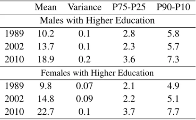
stagnated in some areas (Panels A and B of Figure 2.5). Between 2002 and 2010, the share of ed-ucated male and female population increased universally across regions (Panels C and D of Figure 2.5). The growth in the share of educated individuals occurred together with a growing dispersion of gender-specific human capital across regions. In the 2000s, the share of educated males and females increased more in the regions with the highest share of educated individuals in 2002 (Pan-els C and D of Figure 1.6). Table C.1 shows that the interquartile range of the share of educated males increased from 2.3 percentage points in 2002 to 3.6 percentage points in 2010 and from 2.2 percentage points in 2002 to 3.7 percentage points in 2010 among females. The difference between the 90th and the 10th percentile of the share of population with higher education also increased more rapidly among females and exceeded that of males in 2010. Thus, female human capital became more dispersed across regions over time.6

To graph the relationship between the changes in the educational composition of population and wages over time, Figure 1.7 plots the region-level wage changes against the changes in the fraction of population with higher education in the 1990s and the 2000s. Panels A and B show a negative relationship between the two variables in the 1990s for males and females while Panels C and D show that the relationship became positive in the 2000s. Between 2002 and 2010, regions with the fastest growing share of educated individuals experienced the highest wage increases, and the relationship between the two was stronger for female population.

The faster growth of female college participation resulted in a reversal of the gender gap in higher education in Russia. In 2002, the share of female population with higher education ex-ceeded the share of educated males by 0.8 percentage points (Panel C of Figure 2.1). Between 2002 and 2010, the share of educated females grew faster than that of males, which led to a three-percentage-point gender education gap in favor of females in 2010. The evolution of the gender education gap in the U.S. follows a similar pattern, however, the gap in higher education closed only recently (Panel D of Figure 2.1). Changes in the gender education gap are primarily driven

(17)

by the younger cohorts. However, while in Russia the share of educated young females was al-ready higher than the share of young males in late 1980s, a small gap in favor of educated young males existed in the U.S. in 1990. In Russia, the gender gap in higher education between young individuals tripled from 4 to 12 percentage points between 1989 and 2010 (Panel A of Figure 1.8). Over time, young females in Russia become much more likely than males to receive higher edu-cation. These changes provide motivation for the model which links together changes in the share of male and female population with higher education in a labor market and male and female wages.

1.3 Econometric Framework

1.3.1 Theoretical Model

The goal of the theoretical model is to show how to identify education externalities by gender, i.e., the effect of an increase in the relative supply of educated male and female workers in a labor market on the wages of male and female workers with different levels of education. The model predicts that when the relative supply of educated workers increases, wages of uneducated workers benefit both from imperfect substitution and education externality, while the wages of educated workers decrease because of the increased supply of educated workers but benefit from the education externality.

Assume that a country consists of a number of geographic regions, which represent competitive labor markets.7 Each labor market produces a single goodyand employs educated and uneducated male and female labor and capital. The production is represented by a Cobb-Douglas function8_:

7_{Geographic regions are usually represented by cities(Ciccone and Peri (2006); Conley and Tsiang (2003); Moretti} (2004); Muravyev (2008); Rauch (1993); Sand (2013)), provinces (Bratti and Leombruni (2014)), or states (Acemoglu and Angrist (2001); Ciccone and Peri (2006); Iranzo and Peri (2009); Lange and Topel (2006)).

8_{This form of the production function rules out substitutability between male and female workers in the production.} This assumption is valid if there is high degree of gender segregation across occupations and/or industries. In Russia, women were highly concentrated in some industries, such as education (82% women, 18% men), healthcare (80% women, 20% men), services (70% women, 30% men) in 2012, and not highly represented in other industries, such as construction (15% women, 85% men) and transportation (27% women, 73% men). Compared to the U.S., Russian occupational segregation across genders is higher, which motivates this form of the production function.

(18)

y= X

g=m,f

(θ₀gLg₀)α0₍_θg

1L

g

1)

α1_Kg1−α1−α0 _(1.1)

whereLg₀ is the number of uneducated workers of gendergin a labor market;Lg₁ is the number of educated workers of gendergin a labor market; Kg _{is capital allocated to workers of gender}_g_in a labor market; and theθ’s are gender- and education-specific productivity shifters, which depend on the share of educated workers of gendergin a market:

log(θg₀) = φg₀+µg( L

g

1

Lg₀ +Lg₁), g =m, f (1.2)

log(θg₁) = φg₁+µg( L

g

1

Lg₀ +Lg₁), g =m, f (1.3)

whereφg₀andφg₁capture the effect of gendergworkers’ human capital on productivity and L

g 1

Lg0+L g 1 < 1is the share of gendergworkers with higher education in a labor market. In a competitive market, wages are equal to the marginal product of labor.9

The wages of uneducated workers of gendergare equal to

logw₀g =logα0+α0log(φg0 +µ

g₍ L g

1

Lg₀+Lg₁)) + (α0−1)log(1− Lg₁

Lg₀+Lg₁) (1.4)

+α1log(φg1+µ

g₍ L g

1

Lg₀+Lg₁))( Lg₁

Lg₀+Lg₁) + (1−α1−α0)log( Kg Lg₀+Lg₁)

Wages of educated workers of gendergare equal to

logw₁g =α0log(φg0+µ

g L

g

1

Lg₀ +Lg₁)(1− Lg₁

Lg₀ +Lg₁) +logα1+α1log(φ g

1+µ

g L

g

1

Lg₀+L1

) (1.5)

+ (α1−1)log(

Lg₁

Lg₀+Lg₁) + (1−α1−α0)log( Kg Lg₀+Lg₁)

(19)

Assuming the population size,Lg₀+Lg₁, stays constant (i.e., no demographic shocks), the effect of changes in the share of educated workers of gender gcan be derived by taking the derivative of wages with respect to the share of educated workers of genderg:

∂log(w₀g)

∂ L

g 1

Lg₀+Lg₁

= α0µ

g

φg₀+µg₍ Lg1

Lg₀+Lg₁)

+ 1−α0 1− Lg1

Lg₀+Lg₁

+ α1µ

g

φg₁+µg₍ Lg1

Lg₀+Lg₁)

+ α1

Lg₁ Lg₀+Lg₁

(1.6)

∂log(w₁g)

∂ L

g 1

Lg0+L g 1

= α0µ

g

φg₀ +µg₍ Lg1

Lg0+L g 1)

− α0

1− Lg1

Lg0+L g 1

+ α1µ

g

φg₁+µg₍ Lg1

Lg0+L g 1)

+α1−1

Lg₁ Lg0+L

g 1

(1.7)

Equation (1.6) shows that when the share of male/female workers with higher education increases, wages of uneducated male/female workers increase because 1) uneducated workers’ productivity increases due to the imperfect substitution between workers with different levels of education

1−α0

1− Lg1

Lg₀+Lg₁

+ α1

Lg₁ Lg₀+Lg₁

>0

and 2) there is a positive externality from education

α0µg

φg₀+µg₍ Lg1

Lg₀+Lg₁)

+ α1µ

g

φg₁+µg₍ Lg1

Lg₀+Lg₁) >0

Equation (1.7) shows that the effect on wages of male/female workers with higher education de-pends on two effects: 1) a supply effect, which moves the labor market along a downward sloping demand curve

α1 −1

Lg₁ Lg₀+Lg₁

− α0

1− Lg1

Lg₀+Lg₁ <0

and 2) an education externality effect

α0µg

φg₀+µg₍ Lg1

Lg₀+Lg₁)

+ α1µ

g

φg₁+µg₍ Lg1

Lg₀+Lg₁) >0

Hence, changes in the wages of educated male/female workers in response to an increase in the

(20)

share of educated male/female workers depend on which of the two effects (supply effect or edu-cation externality effect) is stronger.

1.3.2 Empirical Model

This section describes an empirical specification of the wage equation based on the theoreti-cal model derived above and discusses problems associated with estimating education externality effect. The wage of individual iof gender gliving in region r in period t is equal to the market equilibrium wage and is determined by an equation of the form

log(w_irtg ) =βgX_itg +ϕgS_rtg +αgZrt+γr+γt+ugirt, g =m, f (1.8)

whereX_itg is a vector of individual characteristics;S_rtg represents the percentage of college educated workers of gendergin regionrin yeart;Zrtis a vector of characteristics of regionrat timetwhich may be correlated withS_rtg;γrrepresents region fixed effect; andγtis year effect. The error term, ug_irt, is the sum of three components:

ug_irt=ν_rgλ_irg +ξ_rtg +ηg_irt (1.9)

whereλg_ir is a permanent individual unobservable component (e.g., ability);ν_rg is a factor loading which represents the return to the unobserved component λg_ir in region r; ξ_rtg represents time-varying shocks to labor demand and supply in regionrin periodt;η_irtg is the transitory component of log wages which is assumed to be independently and identically distributed over individuals, regions and time.

(21)

an OLS estimateϕˆg is biased either downward or upward, depending on whether the variation in the relative number of educated workers is driven by the unobserved supply or demand factors (Moretti 2004). If the variation in college share across regions is driven by the supply factors, the unobserved heterogeneity biases the OLS estimate downward. This may occur when some unobserved characteristics of the region attract more educated workers to the area raising the share of educated individuals (for example, geographic location, climate, amenities). To get a consistent estimate of the education externality effect, a researcher needs an instrumental variable that is uncorrelated with the region unobserved characteristics but correlates strongly with college share in the region.

On the other hand, an upward bias in the OLS estimate,ϕˆg_{, of the education externality effect} arises from the heterogeneity in the demand for educated workers across regions. In this case, the OLS coefficient in a regression of wages of educated workers on the share of educated workers assigns all of the observed correlation between wages and the share of educated workers to educa-tion externality and yields an estimate that is upward biased. An instrumental variable uncorrelated with factors that affect the productivity of educated workers and, therefore, the demand for them would generate a consistent estimate of education externality.

1.3.3 Identification

The main challenge associated with estimating education externalities is the endogeneity prob-lem arising due to the correlation between the share of college educated workers in the region and wages. Acemoglu and Angrist (2001) is one of the first studies that addresses the endogene-ity problem by using differences in the compulsory schooling and child labor laws across U.S. states as instruments for the average human capital in the labor market. However, the variation in this instrument primarily affects secondary education while sizeable externalities may instead be generated by college education.10 Therefore, recent studies shifted their focus to higher levels of education such as college education. For example, Moretti (2004) uses the age structure of a

10_{For example, Rosenthal and Strange (2008) show that the benefits of spatial concentration are driven by proximity} to college educated workers.

(22)

local labor market in the past and the presence of a land-grant college as the instruments for the share of college graduates and finds sizeable human capital externalities of college education. Dias and Tebaldi (2014) provide evidence that sector concentration of highly qualified workers (with at least a college degree) generates knowledge externalities, i.e., workers learn from their peers. To reconcile the mixed evidence on human capital externalities generated by high school and col-lege education, Iranzo and Peri (2009) develop a model that predicts positive externalities from increased college education and negligible external effects from high school education.

(23)

the demand for skilled labor in the emerging market economy of the 1990s and the 2000s.

1.4 Data

The data for this study comes from the Russia Longitudinal Monitoring Survey (RLMS), a lon-gitudinal survey of the population of Russia initiated in the early 1990s to measure the effect of the market reforms on the economic well-being of the households and individuals.11 _{The distribution}

of the initial sample of households by gender, age, and urban-rural location compared well with the corresponding distribution of the Soviet Census 1989. In later years, the sample was replenished to preserve the representativeness of the population of Russia. RLMS collects a rich set of infor-mation on demographic characteristics, education, health, labor market outcomes, and community characteristics, among many other. This chapter uses sixteen waves of RLMS spanning the period from 1994 to 2011.12 The sample includes 22-59-year old men and 22-54-year old women.13 I drop youths under the age of 22 because some of them may still be completing their education.

Using the Census data, I calculate the share of male and female population with higher educa-tion to proxy for the share of workers with higher educaeduca-tion,S_rtg.14 _{The Census data are}

disaggre-gated by gender, geographic region, age (5-year groups), and the type of residence (urban/rural).15 The share of male/female population with higher education in a region, in a particular age group, and in an urban/rural location is calculated as the number of males/females with complete higher education divided by the total male/female population. This measure is then merged with the RLMS based on the workers’ current region of residence, their age, and the type of location where

11_{RLMS is organized by the National Research University Higher School of Economics, Moscow together with the} Carolina Population Center at the University of North Carolina at Chapel Hill and the Institute of Sociology at the Russian Academy of Sciences. See http://www.cpc.unc.edu/projects/rlms-hse/project/study for the description of the study.

12_{RLMS was not conducted in 1997 and 1999.}

13_{The official retirement age is 55 for women and 60 for men.}

14_{The primary reason for this decision is a lack of data on the share of educated workers across regions and over} time. I assume linear growth and interpolate the share of population with higher education in years for which Census data is not available.

15_{Age groups are 20-24, 25-29, 30-34, 35-39, 40-44, 45-49, 50-54, and 55-59. Urban locations include cities and} townships. Rural locations include villages.

(24)

they live (urban/rural).

Labor market characteristics of regions such as the unemployment rate and the employment by industry and gender come from the Russian Federal Statistical Services. These characteristics are merged with the RLMS based on the respondent’s current region of residence and survey year. They vary both across regions in a given year and over time due to the transition to the market economy during the period of study. The transition was characterized by the changing industrial structure and employment in different industries (Bank (2003), Bank (2005)). For example, the share of employment in manufacturing declined from 27 percent in 1994 to 19 percent in 2011. The share of employment in agriculture, construction, and transportation also declined. On the other hand, the share of employment in trade and education increased over time.

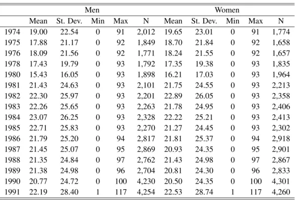
The Russian University Database provides the number of campuses of higher education insti-tutions during the Soviet period (Belskaya and Peter (2015)).16 This database contains detailed information on more than 1,000 institutions of higher education in Russia. Table A.2 shows the distribution of the number of campuses by year. The number of campuses varies considerably over time and across regions. The mean number of campuses per region increased from 19 campuses in 1974 to 22 campuses in 1991. The standard deviation decreased in the 1970s but increased steadily until the 1980s and declined again in the late 1980s.

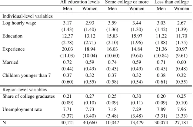
Table A.3 presents the descriptive statistics of three samples used in the empirical analysis: workers of all levels of education, workers with some higher education or more (college dropouts, college graduates, and postgraduate graduates), and workers with less than higher education (sec-ondary school dropouts, sec(sec-ondary school graduates, and specialized sec(sec-ondary education gradu-ates). There are 40,121 male individuals in the sample and 40,660 female individuals. Columns 1 and 2 of Table A.3 present descriptive statistics of the samples of male and female workers. There is a 0.24 log points difference in hourly wages between male and female workers. Average work experience of male workers exceeds the experience of female workers by one year. On the other hand, female workers have 0.75 more years of education and the share of female population with

(25)

higher education in a local labor market exceeds the share of male population by 0.06 percentage points. Columns 3 and 4 present descriptive statistics for the sample of educated workers. There is a 0.15 log points difference in hourly wages, female college graduates have 0.14 more years of education compared to male college graduates, and the share of educated females exceeds the share of educated males by 0.05 percentage points. Columns 5 and 6 present descriptive statistics for the sample of workers without college education. The sample of less educated workers differs from the sample of educated workers in many respects. First, the gender wage gap of 0.36 log points is more than double than the gender wage gap between educated workers. Second, less educated females have 0.48 more years of education than less educated males, which is a three times larger gap compared to the gender gap in education among educated workers.

1.5 Results

1.5.1 Social Returns to Education

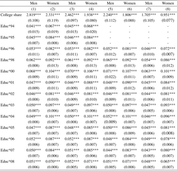
This section presents the estimates of the social returns to education for male and female work-ers as well as the changes in the social returns from mid-1990s to late 2000s. I estimate equation (1.8) by gender and report the results in Table A.4. Individual characteristicsX_irtg include years of education, work experience, and work experience squared. To correct for selection into the labor market, I estimate an inverse propensity weight from the probit model of non-missing wages on individual characteristics and dummies for being married and having children under the age of seven. I use the inverse of the estimated weight in all models. Columns 1 and 2 of Table A.4 show that there is a 2.819 percent increase in wages of male workers and a 2.331 percent increase in wages of female workers in response to a one-percentage point increase in the share of male and female population with higher education. The estimates also suggest that private return to one year of education for female workers exceeds that for male workers throughout the period. Another interesting finding is positive and significant returns to work experience for female workers and negative returns for male workers.

Columns 3 and 4 provide the estimates of the model that controls for the regional unemploy-ment rate which proxies for the time-varying labor demand shocks. The estimates of the social

(26)

returns to education decrease which implies that labor demand shocks matter. In columns 5 and 6, I include regional unemployment rate and an additional control for the labor demand shifts for male versus female labor across industries. Following Katz and Murphy (1992), shifts for male versus female labor across industries are predicted by the nationwide employment growth in industries, weighted by the changes in the region-specific employment share of male and female workers in those industries:

shockgrt =

8

X

i=1

κirt4Egi (1.10)

where i indexes industry; shockgrt represent the predicted employment change for workers of gendergin regionrat timet;κirtis the share of total employment in industryiin regionrat time

t;4Egiis the change in the log of employment in the same industry nationally between 1994 andt by workers of genderg.17 The inclusion of the index lowers the estimates to 2.240 percent for male and 1.806 percent for female workers. The fact that Katz-Murphy index changes the estimates of the external returns to education further supports the idea that the demand shocks may introduce the bias. Therefore, it is important to control for them. Finally, to control for the unobserved permanent region-specific characteristics, I estimate equation (1.8) with the region fixed effects in column 7 and 8. Controlling for the heterogeneity across regions lowers the external returns to education to 1.705 percent for male and 0.951 percent for female workers but the estimates remain statistically significant.

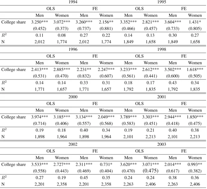
Given that the share of educated individuals grew over time, I estimate changes in the social returns to education by year. Column 1 of Table 2.5 suggests that the returns to college share for male workers increased from 3.250 percent in 1994 to 3.974 percent in 2000 and decreased there-after, reaching a minimum of 1.909 percent in 2011. The returns for female workers followed a similar pattern. Accounting for the heterogeneity across regions in columns 3 and 4 reveals a sim-ilar time trend, however, the returns become lower. The finding that the estimates of social returns from using single cross-sections are considerably larger than the estimates that control for region

(27)

fixed effects suggests that at least part of the relationship between the share of educated individu-als and wages is due to omitted labor markets characteristics. A decline in the external returns to education in the 2000s coincided with an increase in the supply of college-educated workers who entered colleges during the expansion in the 1990s and started to join the labor force in the early 2000s. This finding parallels Sand (2013), who finds declining external returns to education in the U.S. between 1980s and 1990s. It is possible that an increase in the education level of population in a country with high level of educational attainment (such as Russia and the U.S.) decreases the external returns to education. Overall, the analysis in this subsection shows the existence of cor-relations between the main variable of interest, the share of male/female population with higher education, and wages of male and female workers.

1.5.2 External Returns to Education by Education Group

The model presented in Section 3 shows that the external returns to education represent a sum of the imperfect substitution effect and the spillover effect. To identify education externalities, the model needs to be estimated separately for workers with different levels of education. This section presents the estimates the effect of changes in the share of educated males and females on wages of workers with different levels of education.

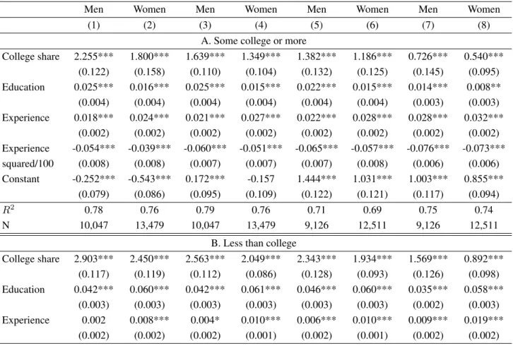
Panel A of Table 2.6 reports the estimates of equation (1.8) for the sample of male and female workers with higher education. The coefficient on the share of population with higher education is found to be positive for skilled workers, implying that the positive education externality ef-fect exceeds the negative supply efef-fect. There is a 2.255 percent increase in wages of educated male workers and a 1.8 percent increase in wages of educated female workers in response to a one-percentage point increase in the share of male and female population with higher education. Accounting for local demand shifts and regional heterogeneity in column 7 and 8 lowers the esti-mates to 0.726 percent for educated males and 0.54 percent for educated females but does not alter the sign and statistical significance of the estimates. In Panel B of Table 2.6, I estimate equation (1.8) for a sample of workers with less than higher education. The estimates support the prediction

(28)

of the theoretical model that the external return associated with an increase in college share is pos-itive for the unskilled workers. Compared to Panel A, the estimates are higher due to the pospos-itive supply effect as indicated by the theoretical model.18

1.5.3 Instrumental Variable Estimates

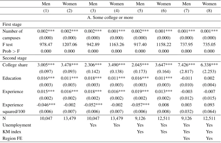
The primary concern associated with estimating education externalities is that the share of educated individuals in the labor market is endogenous. To address the endogeneity concern, I estimate the model using the instrumental variable method. I use the number of college campuses in the region of residence in the past to instrument the contemporaneous share of college educated male and female workers. The results are reported in Table 2.7. The first stage results show that the number of college campuses has a strong and significant effect on the share of individuals with higher education. Compared to OLS estimates presented in Table 2.6, IV estimates are somewhat larger which suggests the presence of a downward bias in the OLS estimates due to the unobserved supply factors driving the variation in the share of educated individuals across labor markets. A one percentage point increase in the share of educated male population implies a 3.005 percent increase in male wages (Column 1). A similar increase in educated female population leads to a 3.478 percent increase in female wages. Controlling for the unobserved demand shocks using local unemployment and Katz-Murphy index lowers these effects to 2.045 percent for male workers and 3.647 percent for female workers (Column 5 and 6). Thus, the yearly increase in the share of male population with higher education of 0.76 percentage points observed in Russia between 2002 and 2010 implies an increase of 1.5 percent in male wages. An increase in the share of educated females of 1.06 percentage points per year observed in Russia between 2002 and 2010 implies a 3.86 percent increase in female wages. A higher increase in female wages during the period of study implies that education externalities contributed to the narrowing of the gender wage gap among educated workers in Russia.

(29)

In columns 7 and 8, I estimate a model that controls for the unobserved heterogeneity across labor markets. The interpretation of the estimates in this specification changes as the main vari-ation in the instrument comes from changes in the number of campuses in a given locvari-ation over time. Therefore, the estimates of 7 percent for male workers and 6 percent for female workers are interpreted as a Local Average Treatment Effect (Imbens and Angrist, 1994).

Panel B of Table 2.7 reports the estimates for a sample of uneducated workers. The IV esti-mates of education externalities in a model that controls for the labor demand shocks suggest a 2.380 percent increase in male and a 3.491 percent increase in female wages in response to a one percentage point increase in the share of educated male and female workers, respectively. Given the annual growth of the share of educated male population by 0.76 percentage points and educated female population by 1.06 percentage points, wages of unskilled male workers increased by 1.8 percent and wages of unskilled female workers increased by 3.7 percent. Compared to the wage increase among educated workers due to the growth in the share of educated male and female pop-ulation, the gender wage gap among unskilled individuals decreased at a slower pace.

1.5.4 Robustness Checks

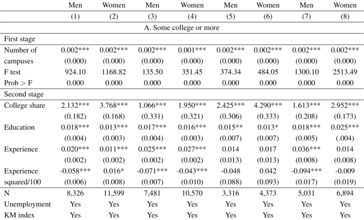
Table 2.8 presents estimation results of the alternative specifications. In Column 1 and 2, I exclude the period of the transition to a market economy and estimate the model limiting the time period to 2000-2011. The estimates of education externality for both male and female workers increase compared to the baseline (Column 5 and 6 of Table 2.7), which implies that the labor mar-kets become more responsive to changes in the educational composition of the labor force com-pared to the transition economy. In Column 3 and 4, I report the estimates when two largest cities, Moscow and St.Petersburg, are excluded from the sample. These cities differ from the remaining regions in terms of educational attainment of the labor force, the number of college campuses, and labor market characteristics. The estimates of education externalities decrease quite significantly highlighting the fact that externalities are probably higher in larger labor markets or markets with high level of educational attainment. In Column 5 and 6, I restrict the sample to individuas who are 25-34-year old as they represent the group with the largest gender education gap in favor of

(30)

females. Finally, in Column 7 and 8, I estimate the model using the sample of individuals older than 35. Compared to the baseline estimate of of education externality of 2.045 percent, younger male workers experience a 2.425 percent increase in their wages when the share of educated male workers increases by one percent. On the other hand, the wages of older male workers would only increase by 1.613 percent in response to such a change. The estimates of education externalities for female workers are also significantly higher for younger females, 4.290 percent compared to 2.952 percent for females older than 35. Overal, Table 2.8 shows that educated female workers younger than 35 working in urban areas receive the largest gains from education externalities.

1.6 Conclusion

This chapter documents the reversal of the gender gap in tertiary education around the world and establishes a causal relationship between the changes in the share of educated male and female population and the gender wage gap through education externalities. In light of the growing female college participation, the analysis of this chapter becomes important for policy makers around the world because an increasing number of educated women will be joining the labor force in the nearest future. Empirical analysis relies on the case of Russia, one of the largest developing countries, which experienced a reversal of the gender gap in higher education over a decade ago. To account for the possibility of the region-wide labor demand shocks that increase wages in a region and attract more educated workers, I estimate these shocks with an index of demand shifts and by the instrumental variable technique. The results suggest that the growth in the share of educated male and female population similar to the one observed between 2002 and 2010 caused the wages of educated male and female workers to grow by 1.5 and 3.86 percent, respectively. Wages of unskilled male and female workers increased by 1.8 and 3.7 percent. Together these changes contributed to the narrowing of the gender wage gap over time

(31)

research in this area.

(32)

Table 1.1: Population with Higher Education by Census Year

Mean Variance P75-P25 P90-P10

Males with Higher Education

1989 10.2 0.1 2.8 5.8

2002 13.7 0.1 2.3 5.7

2010 18.9 0.2 3.6 7.3

Females with Higher Education

1989 9.8 0.07 2.1 4.9

2002 14.8 0.09 2.2 5.1

2010 22.7 0.1 3.7 7.7

(33)

Table 1.2: Number of Campuses of Higher Education Institutions, 1974-1991

Men Women

Mean St. Dev. Min Max N Mean St. Dev. Min Max N

1974 19.00 22.54 0 91 2,012 19.65 23.01 0 91 1,774

1975 17.88 21.17 0 92 1,849 18.70 21.84 0 92 1,658

1976 18.09 21.56 0 92 1,771 18.24 21.55 0 92 1,657

1978 17.43 19.79 0 93 1,792 17.35 19.38 0 93 1,835

1980 15.43 16.05 0 93 1,898 16.21 17.03 0 93 1,964

1981 21.43 24.63 0 93 2,101 21.75 24.55 0 93 2,213

1982 22.30 25.97 0 93 2,201 22.89 26.05 0 93 2,358

1983 22.26 25.65 0 93 2,263 21.78 24.95 0 93 2,406

1984 23.07 26.25 0 93 2,328 22.22 25.21 0 93 2,413

1985 22.71 25.83 0 93 2,270 21.27 24.45 0 93 2,302

1986 21.79 25.20 0 94 2,817 21.81 25.37 0 94 2,918

1987 21.45 25.07 0 95 2,869 20.93 24.35 0 95 2,901

1988 21.35 24.84 0 97 2,762 21.43 24.98 0 97 2,867

1989 21.38 24.98 0 96 2,704 20.81 24.30 0 96 2,833

1990 20.77 24.72 0 100 4,230 20.50 24.35 0 100 4,301

1991 22.19 28.40 1 117 4,254 22.53 28.74 1 117 4,260

Note: years 1977 and 1979 are not listed because RLMS was not conducted in 1997 and 1999.

(34)

Table 1.3: Summary Statistics, RLMS 1994-2011

All education levels Some college or more Less than college

Men Women Men Women Men Women

Individual-level variables

Log hourly wage 3.17 2.93 3.59 3.44 3.03 2.67

(1.43) (1.40) (1.36) (1.30) (1.42) (1.39)

Education 12.37 13.12 15.83 15.97 11.22 11.70

(2.78) (2.71) (2.10) (1.96) (1.88) (1.75)

Experience 20.03 18.94 16.03 14.84 21.36 20.97

(11.03) (10.04) (10.60) (9.64) (10.84) (9.61)

Married 0.72 0.59 0.74 0.59 0.71 0.60

(0.44) (0.49) (0.43) (0.49) (0.45) (0.48)

Children younger than 7 0.37 0.32 0.37 0.32 0.38 0.32

(0.60) (0.55) (0.58) (0.54) (0.61) (0.55)

Region-level variables

Share of college graduates 0.21 0.27 0.25 0.30 0.20 0.25

(0.09) (0.10) (0.09) (0.11) (0.09) (0.10)

Unemployment rate 7.71 7.73 7.18 7.29 7.89 7.96

(3.37) (3.40) (3.48) (3.48) (3.31) (3.33)

(35)

Table 1.4: Estimates of the Education Externalities by Gender

Men Women Men Women Men Women Men Women

(1) (2) (3) (4) (5) (6) (7) (8)

College share 2.819*** 2.331*** 2.462*** 1.938*** 2.240*** 1.806*** 1.705*** 0.951*** (0.108) (0.119) (0.097) (0.080) (0.112) (0.088) (0.105) (0.077)

Educ*94 0.041*** 0.067*** 0.045*** 0.068*** - - -

-(0.015) (0.019) (0.015) (0.020) - - -

-Educ*95 0.045*** 0.084*** 0.046*** 0.084*** - - -

-(0.007) (0.008) (0.006) (0.008) - - -

-Educ*96 0.053*** 0.082*** 0.053*** 0.082*** 0.052*** 0.081*** 0.046*** 0.072*** (0.011) (0.007) (0.011) (0.007) (0.012) (0.007) (0.010) (0.007)

Educ*98 0.062*** 0.092*** 0.061*** 0.092*** 0.065*** 0.092*** 0.054*** 0.086*** (0.008) (0.013) (0.008) (0.013) (0.008) (0.013) (0.006) (0.012) Educ*00 0.068*** 0.104*** 0.070*** 0.106*** 0.071*** 0.107*** 0.063*** 0.101***

(0.009) (0.011) (0.009) (0.011) (0.022) (0.011) (0.007) (0.009) Educ*01 0.047*** 0.090*** 0.046*** 0.088*** 0.048*** 0.090*** 0.045*** 0.084***

(0.009) (0.011) (0.009) (0.011) (0.009) (0.012) (0.006) (0.012) Educ*02 0.046*** 0.081*** 0.046*** 0.081*** 0.046*** 0.081*** 0.044*** 0.081***

(0.008) (0.010) (0.009) (0.010) (0.009) (0.011) (0.006) (0.011) Educ*03 0.050*** 0.097*** 0.049*** 0.097*** 0.050*** 0.097*** 0.047*** 0.093***

(0.007) (0.006) (0.007) (0.006) (0.008) (0.006) (0.005) (0.006) Educ*04 0.049*** 0.101*** 0.050*** 0.101*** 0.052*** 0.101*** 0.046*** 0.096***

(0.008) (0.007) (0.008) (0.007) (0.009) (0.007) (0.007) (0.007) Educ*05 0.047*** 0.087*** 0.048*** 0.085*** 0.050*** 0.086*** 0.045*** 0.081***

(0.007) (0.007) (0.007) (0.008) (0.008) (0.009) (0.006) (0.008)

Educ*06 0.052*** 0.087*** 0.052*** 0.087*** 0.048*** 0.084*** 0.049*** 0.078*** (0.006) (0.007) (0.007) (0.007) (0.007) (0.008) (0.006) (0.006) Educ*07 0.050*** 0.084*** 0.051*** 0.085*** 0.044*** 0.083*** 0.043*** 0.080***

(0.007) (0.006) (0.007) (0.006) (0.007) (0.007) (0.005) (0.007) Educ*08 0.051*** 0.070*** 0.052*** 0.071*** 0.051*** 0.071*** 0.048*** 0.065***

(0.006) (0.008) (0.005) (0.008) (0.005) (0.008) (0.005) (0.007)

(36)

(1) (2) (3) (4) (5) (6) (7) (8)

Educ*09 0.042*** 0.074*** 0.042*** 0.075*** 0.043*** 0.074*** 0.041*** 0.069*** (0.004) (0.007) (0.004) (0.007) (0.004) (0.007) (0.004) (0.005) Educ*10 0.049*** 0.067*** 0.050*** 0.067*** 0.050*** 0.066*** 0.046*** 0.063***

(0.004) (0.005) (0.003) (0.004) (0.003) (0.004) (0.004) (0.003) Educ*11 0.050*** 0.072*** 0.052*** 0.073*** 0.053*** 0.074*** 0.048*** 0.070***

(0.004) (0.005) (0.004) (0.005) (0.004) (0.005) (0.003) (0.004) Exp*94 -0.005*** 0.006** -0.005*** 0.005** - - -

-(0.002) (0.002) (0.001) (0.002) - - -

-Exp*95 -0.001 0.008*** -0.001 0.007*** - - -

-(0.001) (0.002) (0.001) (0.002) - - -

-Exp*96 -0.004 0.009*** -0.004 0.008*** -0.003 0.008*** -0.003 0.006*** (0.003) (0.002) (0.002) (0.002) (0.002) (0.002) (0.002) (0.002) Exp*98 -0.001 0.010*** -0.001 0.009*** -0.001 0.009*** 0.000 0.008***

(0.001) (0.002) (0.001) (0.002) (0.001) (0.002) (0.001) (0.002) Exp*00 -0.002 0.013*** -0.002 0.012*** -0.002 0.012*** -0.001 0.012***

(0.002) (0.002) (0.002) (0.001) (0.002) (0.001) (0.001) (0.001) Exp*01 -0.006*** 0.009*** -0.006*** 0.008*** -0.005*** 0.008*** -0.004*** 0.009***

(0.001) (0.001) (0.001) (0.001) (0.001) (0.001) (0.001) (0.001) Exp*02 -0.008*** 0.007*** -0.007*** 0.008*** -0.007*** 0.008*** -0.005*** 0.009***

(0.001) (0.001) (0.001) (0.001) (0.001) (0.001) (0.001) (0.001) Exp*03 -0.009*** 0.007*** -0.008*** 0.007*** -0.008*** 0.007*** -0.006*** 0.008***

(0.002) (0.001) (0.001) (0.001) (0.001) (0.001) (0.001) (0.001) Exp*04 -0.008*** 0.008*** -0.007*** 0.008*** -0.007*** 0.008*** -0.005*** 0.008***

(0.001) (0.002) (0.001) (0.002) (0.001) (0.002) (0.001) (0.002) Exp*05 -0.008*** 0.007*** -0.007*** 0.006*** -0.007*** 0.006*** -0.005*** 0.006***

(0.001) (0.002) (0.001) (0.002) (0.001) (0.002) (0.001) (0.002) Exp*06 -0.006*** 0.007*** -0.005*** 0.006*** -0.005*** 0.006*** -0.004*** 0.004***

(0.001) (0.001) (0.001) (0.001) (0.001) (0.001) (0.001) (0.001) Exp*07 -0.004*** 0.009*** -0.004*** 0.008*** -0.005*** 0.007*** -0.004*** 0.006***

(0.001) (0.001) (0.001) (0.001) (0.001) (0.001) (0.001) (0.001) Exp*08 -0.003*** 0.009*** -0.003*** 0.008*** -0.003*** 0.008*** -0.002** 0.005***

(37)

(1) (2) (3) (4) (5) (6) (7) (8)

Exp*09 -0.001 0.012*** -0.001 0.010*** -0.001 0.010*** -0.001 0.008*** (0.001) (0.001) (0.001) (0.001) (0.001) (0.001) (0.001) (0.001) Exp*10 -0.001 0.012*** -0.001 0.011*** -0.001 0.010*** -0.000 0.008***

(0.001) (0.001) (0.001) (0.001) (0.001) (0.001) (0.001) (0.001) Exp*11 -0.001 0.011*** -0.001 0.010*** -0.001 0.010*** -0.000 0.008***

(0.001) (0.001) (0.001) (0.001) (0.001) (0.001) (0.001) (0.001) Cons -0.510*** -1.217*** -0.265 -0.887*** 0.370* -0.095 0.153 -0.424***

(0.172) (0.190) (0.180) (0.205) (0.219) (0.165) (0.171) (0.136)

R2 0.78 0.78 0.78 0.78 0.72 0.72 0.76 0.77

N 40,121 40,660 40,121 40,660 35,831 36,889 35,831 36,889

Unemployment Yes Yes Yes Yes Yes Yes

Katz-Murphy index Yes Yes Yes Yes

Region FE Yes Yes

Notes: Dependent variable is log hourly wage. All specifications include year fixed effect. Standard errors, clustered by region and year, are reported in parentheses. The inverse propensity weight from the probit model of non-missing wages is applied in all models. Asterisks denote significance levels: 1 percent (***), 5 percent (**), and 10 percent (*).

(38)

Table 1.5: Cross-Sectional Estimates of External Returns by Gender

1994 1995

OLS FE OLS FE

College share 3.250*** 3.072*** 3.260*** 2.156** 3.352*** 2.821*** 3.604*** 1.431* (0.452) (0.373) (0.737) (0.881) (0.466) (0.457) (0.733) (0.805)

R2 _0.11 _0.08 _0.27 _0.22 _0.14 _0.13 _0.30 _0.27

N 2,012 1,774 2,012 1,774 1,849 1,658 1,849 1,658

1996 1998

OLS FE OLS FE

College share 2.413*** 2.885*** 2.231** 2.247*** 3.233*** 2.612*** 3.502*** 1.618*** (0.531) (0.470) (0.832) (0.607) (0.561) (0.441) (0.600) (0.505)

R2 _0.14 _0.14 _0.33 _0.31 _0.18 _0.17 _0.43 _0.34

N 1,771 1,657 1,771 1,657 1,792 1,835 1,792 1,835

2000 2001

OLS FE OLS FE

College share 3.974*** 3.185*** 3.134*** 2.049*** 3.789*** 3.303*** 2.944*** 1.850*** (0.714) (0.406) (0.557) (0.568) (0.583) (0.451) (0.418) (0.475)

R2 0.19 0.18 0.40 0.34 0.19 0.21 0.40 0.38

N 1,898 1,964 1,898 1,964 2,101 2,213 2,101 2,213

2002 2003

OLS FE OLS FE

College share 3.533*** 2.727*** 2.311*** 0.731* 3.620*** 3.071*** 2.014*** 0.993** (0.558) (0.443) (0.469) (0.404) (0.470) (0.475) (0.617) (0.382)

R2 _0.27 _0.19 _0.45 _0.35 _0.24 _0.24 _0.38 _0.36

(39)

2004 2005

OLS FE OLS FE

College share 3.509*** 3.008*** 2.183*** 1.018** 3.405*** 2.880*** 2.342*** 1.213** (0.477) (0.410) (0.629) (0.400) (0.427) (0.404) (0.473) (0.539)

R2 _0.30 _0.26 _0.41 _0.37 _0.24 _0.23 _0.39 _0.35

N 2,328 2,413 2,328 2,413 2,270 2,302 2,270 2,302

2006 2007

OLS FE OLS FE

College share 2.949*** 2.791*** 1.882*** 1.166*** 2.715*** 2.615*** 1.770*** 1.250*** (0.426) (0.477) (0.448) (0.284) (0.331) (0.479) (0.362) (0.316)

R2 _0.24 _0.23 _0.37 _0.35 _0.24 _0.25 _0.37 _0.38

N 2,817 2,918 2,817 2,918 2,869 2,901 2,869 2,901

2008 2009

OLS FE OLS FE

College share 2.635*** 2.477*** 1.355*** 0.898** 2.335*** 1.751*** 0.984*** 0.436** (0.382) (0.468) (0.382) (0.332) (0.363) (0.413) (0.272) (0.169)

R2 0.27 0.22 0.40 0.37 0.24 0.21 0.38 0.37

N 2,762 2,867 2,762 2,867 2,704 2,833 2,704 2,833

2010 2011

OLS FE OLS FE

College share 2.101*** 1.498*** 0.803*** 0.239 1.909*** 1.557*** 0.709*** 0.452*** (0.364) (0.412) (0.199) (0.166) (0.376) (0.421) (0.223) (0.139)

R2 _0.24 _0.19 _0.37 _0.37 _0.23 _0.19 _0.37 _0.36

N 4,230 4,301 4,230 4,301 4,254 4,260 4,254 4,260

Notes: Dependent variable is log hourly wage. Standard errors, clustered by region, are reported in parentheses. The inverse propensity weight from the probit model of non-missing wages is applied in all models. Asterisks denote significance levels: 1 percent (***), 5 percent (**), and 10 percent (*).

(40)

Table 1.6: Estimates of Education Externalities by Education Group

(1) (2) (3) (4) (5) (6) (7) (8)

A. Some college or more

College share 2.255*** 1.800*** 1.639*** 1.349*** 1.382*** 1.186*** 0.726*** 0.540*** (0.122) (0.158) (0.110) (0.104) (0.132) (0.125) (0.145) (0.095) Education 0.025*** 0.016*** 0.025*** 0.015*** 0.022*** 0.015*** 0.014*** 0.008** (0.004) (0.004) (0.004) (0.004) (0.004) (0.004) (0.003) (0.003) Experience 0.018*** 0.024*** 0.021*** 0.027*** 0.022*** 0.028*** 0.028*** 0.032***

(0.002) (0.002) (0.002) (0.002) (0.002) (0.002) (0.002) (0.002) Experience -0.054*** -0.039*** -0.060*** -0.051*** -0.065*** -0.057*** -0.076*** -0.073*** squared/100 (0.008) (0.008) (0.007) (0.007) (0.007) (0.008) (0.006) (0.006) Constant -0.252*** -0.543*** 0.172*** -0.157 1.444*** 1.031*** 1.003*** 0.855***

(0.079) (0.086) (0.095) (0.109) (0.122) (0.121) (0.117) (0.094)

R2 _0.78 _0.76 _0.79 _0.76 _0.71 _0.69 _0.75 _0.74

N 10,047 13,479 10,047 13,479 9,126 12,511 9,126 12,511 B. Less than college

College share 2.903*** 2.450*** 2.563*** 2.049*** 2.343*** 1.934*** 1.569*** 0.892*** (0.117) (0.119) (0.112) (0.086) (0.128) (0.093) (0.126) (0.098) Education 0.042*** 0.060*** 0.042*** 0.061*** 0.046*** 0.060*** 0.035*** 0.058***

(0.003) (0.003) (0.003) (0.003) (0.003) (0.003) (0.002) (0.003) Experience 0.002 0.008*** 0.004* 0.010*** 0.006*** 0.010*** 0.009*** 0.019***

(41)

(1) (2) (3) (4) (5) (6) (7) (8)

Experience -0.019*** 0.001 -0.022*** -0.006 -0.027*** -0.006 -0.031*** -0.033*** squared/100 (0.005) (0.005) (0.005) (0.004) (0.005) (0.004) (0.005) (0.006) Constant -0.634*** -1.372*** -0.374*** -1.011*** 2.504*** 0.217* 2.168*** 2.334***

(0.084) (0.079) (0.104) (0.100) (0.106) (0.115) (0.083) (0.074)

R2 _0.78 _0.78 _0.78 _0.78 _0.72 _0.72 _0.78 _0.77

N 30,074 27,181 30,074 27,181 26,705 24,378 26,705 24,378

KM index Yes Yes Yes Yes

Region FE Yes Yes

Notes: All specifications include year fixed effect. Standard errors, clustered by region and year, are reported in parentheses. The inverse propensity weight from the probit model of non-missing wages is applied in all models. Asterisks denote significance levels: 1 percent (***), 5 percent (**), and 10 percent (*).

(42)

Table 1.7: Instrumental Variable Estimates by Gender and Education Group

(1) (2) (3) (4) (5) (6) (7) (8)

A. Some college or more First stage

Number of 0.002*** 0.002*** 0.002*** 0.001*** 0.002*** 0.001*** 0.001*** 0.001*** campuses (0.000) (0.000) (0.000) (0.000) (0.000) (0.000) (0.000) (0.000) F test 978.47 1207.06 942.89 1163.26 917.40 1158.22 737.95 735.05 Prob>F 0.000 0.000 0.000 0.000 0.000 0.000 0.000 0.000 Second stage

College share 3.005*** 3.478*** 2.306*** 3.490*** 2.045*** 3.647*** 7.426*** 6.338*** (0.097) (0.093) (0.142) (0.138) (0.173) (0.164) (2.817) (2.253) Education 0.016*** 0.011*** 0.018*** 0.011*** 0.016*** 0.011*** -0.011 0.002

(0.003) (0.003) (0.003) (0.003) (0.003) (0.003) (0.010) (0.004) Experience 0.015*** 0.016*** 0.018*** 0.016*** 0.019*** 0.013*** -0.003 -0.007

(0.002) (0.002) (0.002) (0.002) (0.002) (0.002) (0.012) (0.015) Experience -0.046*** -0.002 -0.052*** -0.002 -0.057*** 0.008 0.003 0.093 squared/100 (0.006) (0.007) (0.006) (0.007) (0.006) (0.008) (0.032) (0.064) N 10,047 13,479 10,047 13,479 9,126 12,511 9,126 12,511

(43)

(1) (2) (3) (4) (5) (6) (7) (8)

B. Less than college First stage

College share 3.388*** 3.842*** 2.733*** 3.276*** 2.380*** 3.491*** -1.050 0.695 (0.059) (0.069) (0.080) (0.089) (0.091) (0.108) (0.679) (1.203) Education 0.034*** 0.056*** 0.038*** 0.057*** 0.040*** 0.055*** 0.044*** 0.058***

(0.002) (0.002) (0.002) (0.002) (0.002) (0.002) (0.003) (0.002) Experience 0.001 0.000 0.003 0.003* 0.006*** 0.001 0.023*** 0.019***

(0.001) (0.001) (0.001) (0.001) (0.001) (0.002) (0.003) (0.007) Experience -0.014*** 0.027*** -0.021*** 0.016*** -0.025*** 0.025*** -0.058*** -0.033 squared/100 (0.003) (0.004) (0.003) (0.004) (0.003) (0.005) (0.006) (0.024) N 30,074 27,181 30,074 27,181 26,705 24,378 26,705 24,378

Unempoyment Yes Yes Yes Yes Yes Yes

Region FE Yes Yes

Notes: All specifications include year fixed effect. The inverse propensity weight from the probit model of non-missing wages is applied in all models. Robust standard errors are reported in parentheses. Asterisks denote significance levels: 1 percent (***), 5 percent (**), and 10 percent (*).

(44)

Table 1.8: Robustness Checks for the Baseline IV Specification

(1) (2) (3) (4) (5) (6) (7) (8)

A. Some college or more First stage

College share 2.132*** 3.768*** 1.066*** 1.950*** 2.425*** 4.290*** 1.613*** 2.952*** (0.182) (0.168) (0.331) (0.321) (0.306) (0.333) (0.208) (0.173) Education 0.018*** 0.013*** 0.017*** 0.016*** 0.015** 0.013* 0.018*** 0.025***

(0.004) (0.003) (0.004) (0.003) (0.007) (0.007) (0.005) (.004) Experience 0.020*** 0.011*** 0.025*** 0.027*** 0.014 0.017 0.036*** 0.014 (0.002) (0.002) (0.002) (0.002) (0.013) (0.013) (0.008) (0.008) Experience -0.058*** 0.016* -0.071*** -0.043*** -0.048 0.042 -0.094*** -0.009 squared/100 (0.006) (0.008) (0.007) (0.010) (0.088) (0.093) (0.017) (0.019) N 8,326 11,599 7,481 10,570 3,316 4,373 5,031 6,894

Unemployment Yes Yes Yes Yes Yes Yes Yes Yes