SCHEDULING IN WIRELESS CELLULAR DATA NETWORKS
Nomesh Bolia
A dissertation submitted to the faculty of the University of North Carolina at Chapel Hill in partial fulfillment of the requirements for the degree of Doctor of Philosophy in the Department of Statistics and Operations Research (Operations Research).
Chapel Hill 2009
Approved by,
Vidyadhar Kulkarni, Advisor
Serhan Ziya, Committee Member
Nilay Argon, Committee Member
Jasleen Kaur, Committee Member
© 2009 Nomesh Bolia ALL RIGHTS RESERVED
ABSTRACT
NOMESH BOLIA: Scheduling in Wireless Cellular Data Networks (Under the direction of Professor Vidyadhar Kulkarni)
This thesis studies the performance of scheduling policies in a wireless cellular data network.
We consider a cell within the network. The cell has a single base station serving a given number
of users in the cell. Time is slotted and the base station can serve at most one user in a given
time slot. The users are mobile and therefore the data transfer rate available to each user
changes from time slot to time slot depending on the distance from the base station and the
terrain of the user.
There are two conflicting objectives for the base station: maximize the data throughput
per time slot, and maintaining “fairness”. To maximize the data throughput, the base station
would like to serve the user with the highest available data rate, but this can lead to starvation
of some users. To ensure “fairness”, no user should be unserved for a “long” time, i.e., users
should be served in a round-robin manner. Although this problem has been studied in the
literature to some extent, existing methods to do this are ad-hoc. Our goal is to derive policies
that have a sound theoretical basis, and at the same time are computationally tractable, are
easy to implement, are fair to all the users and beneficial for the service providers.
We formulate the problem of finding an optimal scheduling policy as a Markov Decision
Process (MDP) and prove some characteristics of the optimal policy. Since solving the MDP to
optimality is infeasible, given the huge size of the problem, we develop heuristic policies called
“index policies”. These policies are based on a closed form “index” for every user that depends
only its own current state. We derive this index using a policy improvement approach based on
Markov Decision Processes. We also compare their performance with existing policies through
simulation. We develop such index policies in two settings: when every user always has ample
data waiting for it to be served (the infinitely backlogged case), and when data arrives for every
Further, we consider the case of users entering and leaving the cell as well, but only from a
simulation perspective.
ACKNOWLEDGEMENTS
I am sincerely grateful to my advisor Professor Vidyadhar G. Kulkarni for introducing me
to the area of stochastic modeling and for his direction and guidance over the past three years.
Words are not enough to express my gratitude for his dedication and encouragement, which
made my dissertation research a truly joyful and rewarding experience. He provided me with
an environment conducive to self-motivated research and one in line with my own interests. His
approach of providing mentoring on matters ranging from very little ones in the beginning to
bigger ones like the broad direction of the dissertation helped me immensely. Besides knowledge,
one important thing he taught and showed me is the persistence to strive for perfection. His
advice of thinking about the problem even while not actually working on it, and deriving the
pleasure that only such intellectual pursuits can provide inspired me to be a scholar and shall
influence and benefit me for the rest of my life.
I would also like to thank my committee members, Professor Serhan Ziya, Professor Nilay
Argon, Professor Jasleen Kaur and Professor Haipeng Shen, for their helpful suggestions on my
research.
Special thanks to Professor Kevin Glazebrook of Lancaster University Management School,
Dr. Siamak Sorooshyari of Alcatel-Lucent and Professor George Shanthikumar of University of
California, Berkeley for discussions and valuable feedback that helped improve the quality of
this work. Further, I also thank one of the reviewers of one of our papers whose persistence led
us to identify an error in our simulation in the dynamic cell case for infinitely backlogged queues.
I would also like to thank Professor Paul H. Zipkin from Duke University and Professor Eda
Kemahlioglu-Ziya for their enlightening courses on inventory management and supply chain
management which greatly broadened my horizons in the area of stochastic modeling. Big
thanks to Professor E. Michael Foster and Professor Serhan Ziya for their advice and support
to me during my research assistantship with them. This research assistantship gave me a glimpse
policy for victims of substance abuse. Professor Foster’s ability to interpret OR in the context
of health policy problem inspired me to apply models in a relevant way to real life situations.
My sincere thanks to Professor Gabor Pataki for introducing me to the area of deterministic
modeling and Professor Edward Carlstein for his encouraging help and priceless advice on my
career development. I have learned a number of effective methods of teaching and accompanying
evaluation from Professor Carlstein.
Thanks to the faculty and staff of our department and my fellow graduate students and
others at UNC who have helped me throughout the years. They made my experience in Chapel
Hill a beautiful and unforgettable one.
Last, but not the least, I would like to thank my parents and my sister for their love and
support over the years and for bearing with my neglect of family duties. This acknowledgement
would be absolutely incomplete without a warm mention of my friends, and mentors in the
various socio-cultural activities with which I have been involved. I would again like to strongly
thank my advisor Prof Vidyadhar Kulkarni without whose invaluable guidance and mentorship
this dissertation would not have been possible.
Table of Contents
List of Tables . . . x
List of Figures . . . xi
1 Introduction . . . 1
1.1 Overview of Cellular Technology . . . 1
1.1.1 History and Present State of Cellular Radio Networks . . . 2
1.1.2 The Working of the Wireless Cellular System . . . 3
1.2 Third Generation - High Speed Data Networks . . . 5
1.3 The Role of Scheduling . . . 7
1.4 Literature Review . . . 8
1.5 Our Contributions . . . 10
I Infinitely Backlogged Queues 12 2 The Model . . . 15
2.1 Motivation . . . 15
2.2 Proportional Fair Algorithm . . . 16
2.3 Formulation as MDP . . . 17
3 Monotonicity of the Optimal Policy . . . 21
3.1 Monotonicity in Age . . . 21
3.2 Monotonicity in Rate . . . 25
4 Index Policy . . . 30
4.1 Policy Improvement Approach . . . 30
4.2 Initial Policy . . . 31
4.3 Policy Improvement Step . . . 34
4.4 Optimizing the Average Reward . . . 38
5 Performance Analysis of LIP and PFA . . . 40
5.1 Introduction . . . 40
5.2 Characteristics of the LIP . . . 41
5.3 Simulation Results . . . 45
5.3.1 The Estimators . . . 45
5.3.2 Simulation Parameters . . . 46
5.3.3 Constant Number of Users . . . 47
5.3.4 Poisson Arrival of Users . . . 48
5.4 Summary . . . 49
II External Data Arrival 54 6 The Model . . . 57
6.1 Motivation . . . 57
6.2 Existing Algorithms . . . 58
6.3 MDP Formulation . . . 60
7 Monotonicity of the Optimal Policy . . . 64
7.1 Monotonicity in Data Queue Lengths . . . 64
7.2 Monotonicity in Rate and Arrivals . . . 69
8 Index Policy . . . 72
8.1 Initial Policy . . . 73
8.2 Policy Evaluation . . . 78
8.3 Policy Improvement Step . . . 81
8.4 Stability of the Index Policy . . . 85
8.5 Aggregate Stability Condition . . . 87
8.6 Variable Number of Users . . . 88
9 Performance Analysis . . . 90
9.1 Introduction . . . 90
9.2 Simulation Results . . . 91
9.2.1 The Estimators . . . 91
9.2.2 Simulation Parameters . . . 92
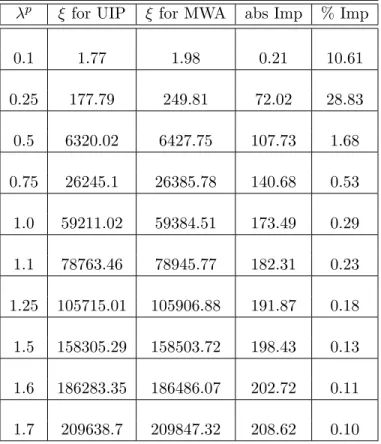
9.2.3 Constant Number of Users . . . 92
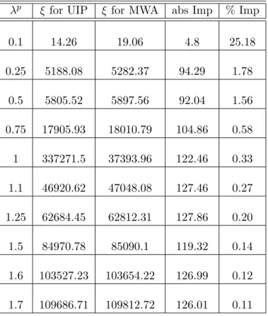
9.2.4 Poisson Arrival of Users . . . 94
10 Conclusions and Future Remarks . . . 96
List of Tables
9.1 Performance of the index policies and the MWA in the static cell . . . 93
9.2 Performance of the index policies and the MWA in the dynamic cell . . . 94
List of Figures
1.1 A Cellular System . . . 4
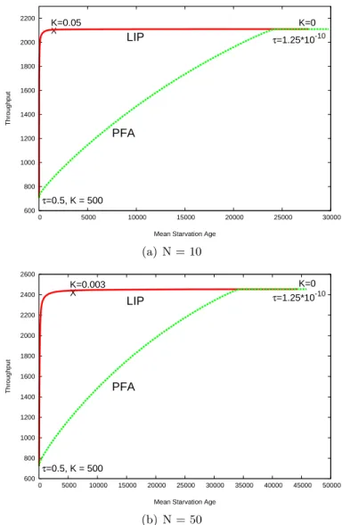
5.1 Throughput Vs Mean Starvation Age: Constant N . . . 50
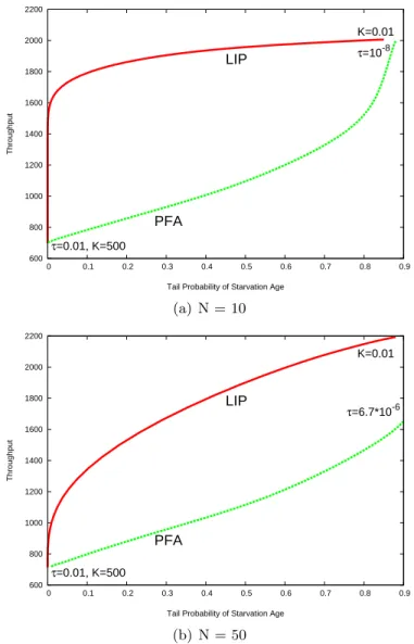
5.2 Throughput Vs Probability of Starvation for≥dslots: Constant N . . . 51
5.3 Throughput Vs Mean Starvation Age: Varying N . . . 52
5.4 Throughput Vs Probability of Starvation for≥dslots: Varying N . . . 53
Chapter 1
Introduction
Wireless Cellular networks have long been used for voice communication effectively. The
proliferation of cell phone usage in the past decade across the world is probably one of the most
visible signs of the advancement of technology. With improvements in the technology, data
transfer over the internet has become an important application of wireless cellular systems.
In fact the revenues from mobile data services reached $188.7 billion in 2008, representing a
24% year-on-year increase according to data sourced from Informa Telecoms & Media’s latest
report [1]. This also means that mobile operators now generate approximately one fifth of their
revenue from data services; a development that is considered significant, given that a general
slowdown in voice revenues is a cause of concern for mobile operators. Further, at the end of
2008 40% of the data revenue was from non-SMS services pointing to the emergence of
ever-newer applications of data services that inevitably require high speed data transmission. An
example of such an application is high speed (broadband) internet surfing on cell phones. With
these futuristic applications in mind, we study ways to improve the performance of high speed
data transmission in wireless cellular networks in this thesis. We begin with a brief overview of
the cellular technology [2].
1.1
Overview of Cellular Technology
Cellular network systems facilitate mobility in communication. These systems achieve
mo-bility by transmitting data through radio waves. Cellular networks derive their name from
to serve. Each cell is serviced by one radio transceiver (transmitter/receiver) called the base
station. The cellular structure of the network enables frequency reuse. Cells, a certain distance
apart, can reuse the same frequencies ensuring efficient usage of limited radio resources [3].
Communication in a cellular network is full duplex, i.e., communication is attained by sending
and receiving messages on two different frequencies and hence at the same time.
1.1.1 History and Present State of Cellular Radio Networks
The first car-based telephone was set up in St. Louis, Missouri, USA in 1946. The system
used a single radio transmitter on top of a tall building. A single channel (frequency) was used
for transmission, therefore requiring a button to be pushed to talk, and released to listen [3].
Such a system, referred to as a half duplex system (as opposed to a full duplex system like
the current cellular networks), is still used by modern day CB radio systems utilized by police
and taxi operators. In the 1960s, the system was improved to a two-channel system called the
improved mobile telephone system (IMTS) [3]. Since frequencies were limited, the system could
not support many users.
Cellular radio systems, implemented for the first time in the advanced mobile phone system
(AMPS), support more users by allowing reuse of frequencies. AMPS is an analog system, and
a part of first generation (1G) cellular radio systems. In contrast, second generation systems
are digital. In the USA, two standards were introduced for second generation systems: IS-95
(popularly known as CDMA, acronym for Code Division Multiple Access - the technology used
for digital data transfer) and IS-136 (popularly known as D-AMPS and based on Time Division
Multiple Access, i.e., TDMA - again, another technology like CDMA for communication) [3,
4]. Europe consolidated to one system called the global system for mobile communications
(GSM, based on TDMA) [4]. Even in the US, most mobile operators working with the TDMA
technology have migrated to GSM. Japan uses a system called personal digital cellular (PDC)
that works on a technology similar to GSM.
Today Cellular radio is the fastest growing segment of the communications industry [3].
According to GSMA, an international mobile communications industry group, the total number
of cell phone subscribers recently crossed the four billion mark and is expected to reach six billion
Current cellular radio systems are in their second generation (2G). The third generation
of cellular systems (3G systems) will allow different systems to interoperate in order to attain
global roaming across different cellular radio networks as well as allow new applications such as
high speed internet surfing, multimedia messaging and video conferencing [6]. The International
Telecommunication Union (ITU) has been doing research on 3G systems since the mid 1980s.
Their version of a 3G system is called international mobile telecommunications - 2000
(IMT-2000).
European countries are researching 3G systems under the auspices of the European
Commu-nity [6]. Their system is referred to as the universal mobile telecommunication system (UMTS),
having the same goals as the IMT-2000 system. 3G systems have the following major objectives:
• Use of common global frequencies for all cellular networks and worldwide roaming.
• High transmission rates for data based services.
• Efficient bandwidth utilization schemes.
1.1.2 The Working of the Wireless Cellular System
In this section, we briefly explain how a wireless celluar network works [2]. In the rest of
this section, a cell phone or any other device that can connect to a cellular radio network will
be referred to as a mobile station in keeping with the literature on the subject.
A cellular network consists of both land and radio based sections. Such a network is
com-monly referred to as a PLMN - public land mobile network [3]. The network is composed of
the following entities:
• Mobile station (MS): A device used to communicate over the cellular network.
• Base station transceiver (BST): A transmitter/receiver used to transmit/receive signals
over the radio interface section of the network.
• Mobile switching center (MSC): The heart of the network which sets up and maintains
calls made over the network.
• Base station controller (BSC): Controls communication between a group of BSTs and a
single MSC.
• Public switched telephone network (PSTN): The land based section of the network.
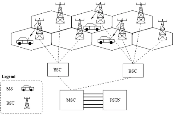
Figure 1.1 illustrates how these entities are related to one another within the network. The
BSTs and their controlling BSC are often collectively referred to as the base station subsystem
(BSS). As explained before, the cellular topology of the network is a result of limited radio
bandwidth. In order to use the radio spectrum efficiently, the same frequencies are reused
in nonadjacent cells. A geographic region is divided up into cells. Each cell has a BST that
transmits data via a radio link to MSs within the cell. A group of BSTs are connected to a
BSC. A group of BSCs are in turn connected to a mobile switching center via microwave links
or telephone lines. The MSC connects to the public switched telephone network, which switches
calls to other mobile stations or land based telephones.
Figure 1.1: The components of a cellular network and their relation to each other
The following description of one mobile station placing a call to another mobile station best
explains the underlying technology of a cellular network system: a mobile station places a call
by sending a call initiation request to its nearest base station. This request is sent on a special
channel, the reverse control channel (RCC). The base station sends the request, which contains
the telephone number of the called party, to the MSC. The MSC validates the request and uses
the number to make a connection to the called party via the PSTN. It first connects itself to
placed the call to switch to voice channels. The mobile station that placed the call is then
connected to the called station [7].
The steps explained above happen fast enough that the user does not experience any
no-ticeable delay between placing a request for a call and the call being connected. The available
frequency is accessed by different users in a cell using one of the two technologies mentioned in
section 1.1.1: TDMA and CDMA. In the TDMA technology, a frequency band is divided into
time slots. Each user gets the radio in this band all to itself for the entire time slot in which it
is served. This is possible in 2G cellular systems (and wasn’t in the 1G analog systems) because
voice data that has been converted to digital information is compressed so that it takes up
sig-nificantly less transmission space. The GSM standard uses TDMA for voice transfer. CDMA
takes an entirely different approach to the use of the available bandwidth. After digitizing data,
CDMA spreads it out over the entire available bandwidth. Multiple calls are overlaid on each
other on the channel, with each assigned a unique sequence code (hence the “code” in CDMA).
Thus data is sent in small packets over a number of discrete frequencies available for use at any
time in the specified range.
As described in the beginning of this chapter, however, voice communication is not the only
service sought by users. Data applications such as web browsing, downloading files from the
internet, multimedia messaging are catching up fast and might soon overtake voice
communica-tion as the prime revenue generator. The 2G systems are inadequate to handle the requirements
of such bandwidth intensive and rate sensitive data applications. The next generation of
wire-less cellular systems that support such applications and are currently the state-of-the-art in the
industry (still being developed and deployed in newer markets) use the 3G technology.
1.2
Third Generation - High Speed Data Networks
The third generation, or 3G as it is popularly called, technology is the latest in mobile
communications. 3G networks have potential transfer speeds of up to 3 Mbps (about 15
sec-onds to download a 3-minute MP3 song). For comparison, the fastest 2G phones can achieve
up to 144Kbps (about 6 minutes to download a 3-minute song). 3G’s high data rates are
ideal for downloading information from the Internet and sending and receiving large,
dia files. 3G phones are like mini-laptops and can accommodate broadband applications like
video conferencing, receiving streaming video from the Web, sending and receiving faxes and
instantly downloading e-mail messages with attachments. 3G comprises several cellular access
technologies. The three most common are:
• WCDMA (UMTS) - Wideband Code Division Multiple Access; versatile and complicated
implementation, hence technically challenging.
• TD-SCDMA - Time-division Synchronous Code-division Multiple Access; currently being
developed by Chinese Academy of Telecommunications Technology and Siemens.
• CDMA2000 - primarily developed to work with existing 2G CDMA carriers; technology
implemented by Qualcomm and currently offered by Verizon wireless and Sprint Nextel
among almost seventy service providers all over the world.
In this thesis we analyze and attempt to enhance the performance of an implementation
of the CDMA2000 technology called Evolution-Data Optimized (EV-DO). It has been adopted
by many mobile phone service providers around the world, particularly, but not only, those
previously employing CDMA networks. An EV-DO channel has a bandwidth of 1.25 MHz, the
same bandwidth size as IS-95 [8]. The end user purchases an EV-DO modem (often referred
to as an “aircard”) that receives the signal and allows connection to the internet. The possible
download speeds vary from 38 Kbps to 2400 Kbps (or 3000 Kbps in a revised implementation
of EV-DO) depending on the user conditions and distance from the base station. The back-end
network is entirely packet-based and employs time multiplexing for data transfer. Thus, time
is slotted (with a slot length of 1.67 milliseconds) and in every time slot each MS sends a pilot
signal to the BST. The strength of the pilot signal depends on the distance of the MS from the
base station, the terrain and other environmental conditions. There are eleven (or thirteen in
the revised implementation of EV-DO) potentially available data rates to users for which the
physical infrastructure is designed. Using the pilot signal the BST determines the rate at which
data can be transmitted to a user if it is chosen to be served. The BST can serve at most one
The first requirement of achieving such high speeds is better infrastructure that includes a
combination of more available bandwidth, more powerful signals and taller base station towers.
However, to be successful commerically the new technology should supplement the existing 2G
systems and work within the existing cellular framework. Hence the mechanism of data transfer
broadly remains the same - using the BST, MSC and the PSTN. One reason for the popularity
of EV-DO among service providers is its complete backward compatibility with CDMA (IS-95)
and the fact that it can be deployed alongside a wireless carrier’s voice services. This makes
EV-DO the most widely used 3G technology currently.
1.3
The Role of Scheduling
Electronics and communication engineers world over are thus working on faster, better
(quality) and cheaper technology to cater to the growing data services market. However better
engineering and technology alone do not ensure effective utilization of the available resources.
We require efficient algorithms to ensure data flow from the base station, the fundamental
transmission unit of cellular networks, to various users fairly and efficiently. In particular we
require effective scheduling policies that determine which users should be served in a given time
slot among all those present in the wireless cell. There are two conflicting objectives for the base
station: maximize the data throughput per time slot, and maintain “fairness”. To maximize
the data throughput, the base station would like to serve the user with the highest available
data rate, but this can lead to starvation of some users. To ensure “fairness”, no user should
be unserved for a “long” time, i.e., users should be served in a round-robin manner. This is the
conflict that we seek to resolve in this thesis. The goal is to determine scheduling policies that
address this conflict, are easy to implement and improve upon the policies that exist currently.
We focus on the downlink (base station to mobile) channel throughout, since in many
applications such as web browsing, most of the data flow occurs in that direction. However all
the ideas presented here can be applied to data transfer in the uplink direction as well.
1.4
Literature Review
The problem of scheduling users for data transmission in a wireless cell has been considered
in the literature mostly in the last decade and a half. One of the most widely used algorithms
that takes advantage of multiuser diversity (users having different and time-varying rates at
which they can be served data) while at the same time being fair to all users is the PFA
of Tse [9]. It is described in detail in section 2.2. In the setting of infinitely backlogged
queues, the PFA performs well and makes good use of the multiuser diversity. This has been
demonstrated in [10] where Jalali et al show using simulation that the throughout per cell of the
wireless network increases as the number of users goes up. A drawback of using this algorithm,
however, is its underlying assumption of unlimited data waiting to be served for each user. It
has been proven to be unstable when there is external data arrival [11] for the users. This
instability in the external data arrival regime is expected because the PFA doesn’t take the
data queue length of users into account while making the scheduling decision. Algorithms that
consider the queue length in making the decision have also been proposed in the literature.
Many such algorithms have theMax-Weight Algorithm (MWA) as their motivation. The
MWA, variously referred to as the Differential Backlog algorithm, the Backpressure algorithm
and the Load Balancing algorithm, was introduced by Awerbuch and Leighton in [12, 13] and
by Tassiulas and Ephremides in [14, 15]. Tassiulas and Ephremides introduce the algorithm
for a multihop radio network and prove its stability in [14]. They consider an extension to
the case of randomly varying connectivity in the network in [15]. A significant amount of work
has since appeared on proving the stability of algorithms similar to the MWA such as Neely
et al [16]. They consider power allocation in a satellite that transmits data to different ground
locations each having a channel of its own. Andrews, Jung and Stoylar [17] prove the stability
of the MWA for dynamic networks. They consider the problem of combined packet routing and
scheduling in communication networks that have high loads and can have dynamically varying
connectivity along any edge of the network. The MWA has also been studied in other situations
such as scheduling input-queued crossbar switches [18], load balancing tasks in a network of
processors [19] and maximizing the total utility of traffic injected into the network [20].
mobile user is governed by a stationary stochastic process such as an erdogic Markov chain.
The MWA has been proved to be stable under this assumption in a variety of settings as
described above. Andrews and Zhang [21] focus on scheduling algorithms that perform well
for nonstationary wireless channels. They show that the MWA performs extremely poorly for
nonstationary channels with an example of a setting under the standard EV-DO infrastructure
where the MWA produces queues that are exponential in the number of users. They present
the Quadratic Tracking algorithm in [22] and prove that the bound on the queue size for this
algorithm is linear in the number of users. In [21] they improve the algorithm and show how
it can be implemented in practice with some approximations where needed.
There also exists literature that deals in algorithms similar to the MWA for scheduling in
wireless networks with time varying channel rates. Andrews et al [23] consider a variant of the
MWA where they also take into account the head of the line packet delay in addition to each
queue length. They call it the Modified Least Weighted Delay First (MLWDF) algorithm and
prove its stability. Shakkottai and Stolyar [24] present another variant of the MWA that they
call the Exponential Rule and prove its stability. We describe each of these algorithms including
the MWA briefly, but precisely, in section 6.2. Further, in [25] they prove that in a heavy traffic
limit and under some more conditions, the exponential rule minimizes maxuauQu(n) whereau
is some positive number, and Qu(n) is the queue length in time slot n of user u. A related
area of reserch is “Generalized processor sharing” (GPS) where a multitude of users share
the capacity of congested communications links in a fair manner. Mainly starting with the
PhD dissertation of Parekh [26], there was tremendous activity and interest in this area [27,
28]. Several algorithms such as Weighted Fair Queuing [29], Start-time Fair Queuing [30] and
Stochastic Fair Queuing [31] have been proposed to keep the queue lengths “’fair” for every
user. In this setting, however, throughput is not a matter of concern since the available data
rate for a user is bounded above only by the entire capacity of a link, and the data transmission
rate does not change due to user mobility. In the wireless cell considered in this thesis, user
mobility and the consequent multi-user diversity gain in throughput motivates us to look for
alternative models and scheduling algorithms.
1.5
Our Contributions
We consider two types of cells according to user movement between cells. We first derive
our scheduling policy assuming a fixed number of users in the cell, and no user movement in or
out of the cell (the users are mobile within the cell). We call such a cell for which the number
of users is fixed a “static cell”. Then we extend the results of a static cell to the case when
users can enter and leave the cell. We refer to such a cell with incoming and outgoing users as
a “dynamic cell”. As discussed in section 1.4, algorithms for scheduling in the static cell have
been studied quite extensively in the wireless networks literature. We extend this work in two
directions: First, the existing algorithms do not explicitly attempt to optimize any system wide
objective function. We develop a Markov Decision Process (MDP) framework to find scheduling
policies that optimize such an objective function. This objective function captures the conflict
between throughput maximization and fairness to users effectively using appropriate costs and
rewards. The policy improvement algorithm (PIA) is then used on the MDP formulation to
derive “index policies” that involve computing an index for each user dependent on the current
state of that user. In any given time slot the index policy serves the user with the highest index.
The index has a sound theoretical basis, and we develop a closed form expression for it so that it
is computationally efficient. We expect better performance from such a policy given its origins
in a sound optimization framework and demonstrate the same through simulations. Secondly,
we develop analytical results when possible and also look at simulations in the dynamic cell
to get an insight into the performance of scheduling policies in a more realistic environment.
To the best of our knowledge, there doesn’t exist any study - numerical, simulation-based, or
analytical - for dynamic cells.
The thesis is divided into two parts, each of which considers one of the two cases according
to the data to be served: “infinitely backlogged” data queues and data queues fed by “externally
arriving” data. The scheduling problem when there is always ample data to be served to every
user is referred to as the “infinitely backlogged” queues case. This is a realistic assumption in
the high congestion regime, where every user has high rate of data arrival and thus always has
data to receive. The objective function that the MDP maximizes in this setting is the long run
transmitted to the user scheduled to be served minus the penalty incurred by users that are not
served. Thus our policy aims to strike a good balance between the two conflicting objectives:
maximizing throughput and maintaining fairness. Part I of this thesis gives a precise account
of these issues and the way we address them. Chapter 2 describes the model of underlying
channel processes and develops an MDP model for the scheduling problem. Chapter 3 discusses
some characteristics of the optimal policy of the MDP. Since the MDP is too complicated to
be solved optimally, we derive several index policies to schedule users in chapter 4. These
policies are based on the standard policy improvement method for Markov Decision Processes.
The proportional fair algorithm, introduced in (PFA) [9], is currently used in practice in these
settings. It has good “fairness” properties [32] but is not based on any systematic “optimization”
procedure to maximize throughput. Therefore we expect that the policies we develop using our
proposed methodology will exhibit better performance. We conclude part I with a performance
analysis of our index policies and the PFA. We demonstrate through simulation that our index
policies result in significantly better performance.
In Part II we consider the case where data arrives for every user randomly. In this case
the throughput for every user is fixed in the steady state, and hence the goal of the MDP is
to minimize the long run total weighted data queue length in a time slot across all users. We
derive the scheduling policy as follows: we describe the model of underlying channel processes
and develop an MDP model for the scheduling problem in Chapter 6. Chapter 7 discusses some
characteristics of the optimal policy of the MDP. As in part I the MDP is too complicated to
be solved optimally, hence we derive some index policies to schedule users in chapter 8. We
Part I
List of Notations for part I
(in the order of appearance)
N - Total number of users
u - Label for the users,u= 1,2, . . . , N
Rn
u - Channel rate of user u
Rn- The vector [Rnu :u= 1,2, . . . , N]
Qu - Exponentially filtered average data rate updated according to equation 2.1
τ - Key Parameter of the PFA, acts as damping coefficient in equation 2.1, PFA throughput
increases as τ decreases
Xn
u - State of user u at timen
M - The number of states in the state space of the DTMC {Xn
u,n≥0} foru= 1,2, . . . , N
Pu - The Transition probability matrix of the Markov chain{Xn
u,n≥0}; has elements [puiu,ju]
Xn = [Xn
1, . . . , XNn] - State vector of all users
i= [i1, i2, . . . , iN] - A realized value of the state vectorXn
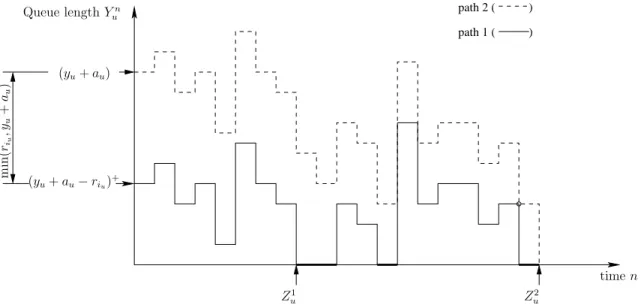
Yn
u - “Starvation age” (or “age”) of the user u at timen
Yn = [Yn
1 , . . . , YNn] - The age vector at timen
t= [t1, t2, . . . , tN] - A realized value of the age vectorYn
A - Action space{1,2, . . . , N} in any state (i, t)
v(n) - User served in thenth time slot
Ω - State space of the DTMC{Xn
u,n≥0}; is same for all usersu= 1,2, . . . , N
r - A constant vector of data rates = [r1, r2, . . . , rM]; whenXun=k,Rnu =rk
Dl(y) - Cost of not serving user lof age y in slotn
VT(i, t) - Optimal reward starting from state [X0, Y0] = [i, t] at time 0 over time periods
0,1,2, . . . , T
g - The long run average throughput
w(i, t) - Bias function starting in state (i, t)
q - Initial policy vector = [q1, q2, . . . , qN]
gq - The constant g under the initial policyq
wq(i, t) - The bias functionw(i, t) under the initial policy q
πu = [πu
1, . . . , πuM] - Steady state distribution of the Markov chain{Xun:n≥0}
φu(qu) - Long run cost per slot for useruunder policy q
Au - Mean reward earned by useru if served in every slot
Ku - Parameter of the LIP for user uso that Du(n) =Kun
Iu(i, t) - The index for user uin state (i, t)
Lq - Lagrangian used to compute the optimal initial policy
θ - Lagrangian multiplier for optimizingLq
B - Long run expected throughput per time slot
ζ - Long run expected starvation age of a user
ρd - Long run probability that a user is starved for more than dtime slots
ˆ
B - Estimate ofB obtained from simulation
ˆ
ζ - Estimate of ζ obtained from simulation
ˆ
ρd - Estimate ofρdobtained from simulation
K - The constantKu assumed the same (K) for all users u
N(t) - Number of users at timet in the cell in the dynamic case
λ- The arrival rate of users in the dynamic cell
Chapter 2
The Model
2.1
Motivation
We start by considering a fixed set of N mobile data users in a wireless cell served by a
single base station. As noted in section 1.3 we focus on the downlink channel. The base station
maintains a separate queue of data for each user. Time is slotted and in each time slot the
base station can transmit data to exactly one user. Let Rn
u (u = 1,2, . . . , N;n = 0,1, . . .) be
the channel rate of user uduring time slotn, i.e., the amount of data that can be transmitted
to user u during time slot n by the base station. We assume that the base station knows at
all time slots n a vector Rn = [Rn
1, Rn2, . . . , RnN]. How this information is gathered depends
on the system in use. An example of a resource allocation system widely known and used
in practice is the CDMA2000 1xEV-DO system [33] described briefly in section 1.2. A good
description of how this information is generated is also provided in [33]. The algorithms
pre-sented in this chapter do not require the details of this mechanism of information transfer. We
simply assume that {Rn,n≥0} is a stochastic process that accounts for the random variation
in data rates due to user mobility and other factors such as user terrain. A good framework
for resource allocation and related issues in this (and more general) setting can be found in [34].
There are two objectives to be fulfilled while scheduling the data transfer. The first is to
obtain a high data transfer rate. This can be achieved by serving a user u in slot n whose
channel rateRn
u is the highest, i.e., following a myopic policy. However if we follow the myopic
The second objective is to ensure that none of the users is severely starved. Thus these are
conflicting objectives and any good algorithm tries to achieve a “good” balance between the
two. An algorithm that seeks to allocate resources to maximize system throughput under
some Quality of Service (QoS) constraints that ensure a certain level of fairness to each user is
presented in [35]. We shall comment on this algorithm later in section 5.4. The key features
of the problem are a stochastic evolution of the data rate available to users, choosing a user to
serve, a reward from serving that user in the form of data served, and a penalty in the form
of unserved hence unsatisfied users. Markov Decision Processes (MDP) models are frequently
used to determine optimal decisions (such as the user to serve) in a stochastic environment.
Further we know that this type of reward structures can be easily incorporated into such
models. A problem with using such a model is the curse of dimensionality if the model is to
be solved to optimality. However previous experience [36] suggests that using only one step of
the policy improvement approach can yield policies that are nearly optimal and do not suffer
from this curse of dimensionality. Derivation of such policies does not need the solution to
the corresponding high-dimensional MDP. This motivates us to develop our MDP and policy
improvement based approach in this chapter. To our knowledge, no past work deals with this
problem using an MDP based approach to derive implementable policies.
The rest of the chapter is organized as follows. In section 2.2 we describe a popular algorithm
called Proportional Fair Algorithm (PFA) currently in use in the 1xEV-DO system. In section
2.3 we formulate the bandwidth allocation problem as an MDP under the assumption of a fixed
number of users in the cell.
2.2
Proportional Fair Algorithm
The Proportional Fair Algorithm [32] is currently used in the 1xEV-DO system. In this part
of the thesis we consider the case where every user has infinitely backlogged queues. This is a
realistic assumption in heavy traffic regime, where every user always has data to receive. The
PFA algorithm implicitly makes this assumption by not considering the current queue length
in choosing which user to serve, and this makes comparison of our policy (derived with an
The PFA aims to optimize a given function of the throughput achieved by all the users. A
commonly used objective function is the Proportional Fair metric P
ulogQu, where Qu is a
given measure of the long term throughput achieved by user u. A useful characteristic of this
metric is that although it is strictly increasing in the throughput of each user, it prevents any
user from being starved since log Qu → −∞asQu →0. The PFA is characterized by a single
constant τ ∈ (0,1) as explained below. Assume that there are a fixed number N of users in
the cell. Letv(n) be the user served in slot n. For each useru, defineQu(0) = 1, and compute
Qu(n) recursively as follows:
Qu(n+ 1) =
(1−τ)Qu(n) +τ Rnu ifu=v(n)
(1−τ)Qu(n) ifu6=v(n),
(2.1)
see [32]. Mathematically,τ acts as a damping coefficient andQu(n) represents an exponentially
filtered average service rate. The constanttc = 1τ can also be taken to be a measure of the time
a user can remain unserved [10]. Clearly Qu(n) represents an exponentially filtered average
service rate. The PFA algorithm chooses to serve userv(n) in slot nwhere
v(n) = arg max
u
Rn
u
Qu(n)
. (2.2)
It can be proved that this algorithm maximizesP
ulogQu(n+ 1) -PulogQu(n) for eachn[32].
The PFA can also handle users of more than one type by assigning different values of τ to
different types of users. It can be seen that users with higher values of τ will be served more
frequently. In the next section we describe our MDP model to make this scheduling decision
optimally.
2.3
Formulation as MDP
In this section we start with a stochastic model for {Rn,n≥0} and formulate the scheduling
problem as an MDP. Let Xn
u be the state of user u at time n. This represents all the various
factors such as the position of the user in the cell, the propagation conditions etc that determine
the data rate received byuin time slotn. We assume that{Xn
u,n≥0}is an irreducible Discrete
Time Markov chain (DTMC) on state space Ω = {1,2, . . . , M} with Probability Transition
Matrix (PTM)Pu = [pu
iu,ju]. We make this assumption to make the analysis tractable [32]. For
the sake of notational convenience, particularly in chapters 3 and 7, we assume, without loss of
generality, that
r1 ≤r2≤. . .≤rN (2.3)
Further, as indicated in section 5.3.2, a set of M = 11 fixed data rates is what is available to
users in an actual system [33]. Letrk be the fixed data rate (or channel rate) associated with
statek∈Ω of the DTMC. WhenXn
u =k, the user u can receive data from the base station at
rate Rn
u =rk.Thus for allu∈ {1,2, . . . , N}, the state space of the Markov chain {Run:n≥0}
isr = [r1, r2, . . . , rN]. LetN be the total number of users in the cell (assumed constant in this
section) and letXn= [Xn
1, . . . , XNn] be the state vector of all the users. Since each component
of {Xn, n ≥0} is an independent DTMC on Ω, it is clear that{Xn,n≥0} itself is a DTMC
on ΩN. We assume the users behave independently of each other and that each user has ample
data to transmit.
Let Yn
u be the “starvation age” (or simply “age”) of the user u at time n, defined as the
time elapsed (in number of slots) since the useruwas served most recently. Thus, the age of the
user is zero at timen+ 1 if it is served in thenth time slot. Furthermore, form≥1, if the user
was served in time slotnand it is not served for the next mtime slots, its age at timen+mis
m−1. LetYn= [Yn
1 , . . . , YNn] be the age vector at timen. The base station serves exactly one
user in each time slot. In this and the following sections let v(n) be the user served in the nth
time slot. It should be noted here that the expression for v(n) given by (2.2) is used only for
the PFA, it does not define v(n) as used in this section. The age variables change according to
Yn+1
u =
Yn
u + 1 if u6=v(n)
0 ifu=v(n)
(2.4)
The “state of the system” at timenis given by [Xn, Yn]∈ΩN×ZN , whereZ ={0,1,2, . . .}.
The “state” is thus a vector of 2N components and we assume that it is known at the base
N users in the time slotn. We need a reward structure in order to make this decision optimally.
We describe such a structure below. If we serve user u in the nth time slot, we earn a reward
ofRn u =rXn
u for this user and none for the others. In addition, there is a cost ofDl(y) if userl
of agey is not served in slotn. Clearly, we can assume Dl(0) = 0 since there is no starvation
at age zero. The net reward of serving useru at timen is
Rnu−X
l6=u
Dl(Yln). (2.5)
We assume that there is no cost in switching from one user to another from slot to slot. This is
not entirely true in practice, but including switching costs in the model will make the analysis
intractable. For convenience we use the notation
Wun=X
l6=u
Dl(Yln).
The problem of scheduling a user in a given time slot can now be formulated as a Markov
De-cision Process (MDP). The deDe-cision epochs are{1,2, . . .}. The state at timenis [Xn, Yn] with
Markovian evolution as described above. The action space in every state isA = {1,2, . . . , N}
where action u corresponds to serving the user u. The reward in state [Xn, Yn]
correspond-ing to action u is Rn
u −Wun. Let the transition probability under action u from (i, s) to (j, t)
(i, j∈ΩN and s, t∈ZN) be denoted by p((j, t)|(i, s), u). It is given by
p((j, t)|(i, s), u) =
p1i1,j1p2i2,j2. . . pNiN,jN =pij,
iftu = 0 andtl=sl+ 1 forl6=u
0 otherwise.
(2.6)
The state space of this MDP, i.e., ΩN ×ZN, is very large which makes the derivation of the
optimal policy extremely hard and unusable in practice. The advantage of our analysis is
that it avoids having to solve the MDP equations. Instead it uses just one step of the policy
improvement algorithm that avoids the curse of dimensionality and produces simple scheduling
policies that have minimal parameter requirements and are unaffected by the size of this state
space. Thus we see that although we start with formulating the problem as an MDP, our final
index policy is independent of the transition probabilitiespu
iu,ju (u=1,2,. . . ,N). We do however
usepu
iu,juto simulate the underlying Markov chain to do a performance analysis of our proposed
policy and the arguments used to obtain the value of pu
iu,ju are described in detail in section
5.3.2. The method described in [37] can also be used to estimate pu
iu,ju based on engineering
considerations, if needed.
Let VT(i, t) be the optimal reward starting from state [X0, Y0] = [i, t] at time 0 over time
periods 0,1,2, . . . , T. If useru is served at time 0, the age vector in the next time slot is given
by
tu = (t1+ 1, . . . , tu−1+ 1,0, tu+1+ 1, . . . , tN+ 1). (2.7)
We also define
Wu(t) =
X
l6=u
Dl(tl). (2.8)
A standard Dynamic Programming (DP) argument then yields the following Bellman equation
VT(i, t) = max
u=1,2,...,N
riu−Wu(t) +
X
j
pijVT−1(j, tu)
, (2.9)
where pij is as defined in (2.6). We wish to determine the action u = u(i, t) that maximizes
limT→∞VT(i, t)/T, i.e., the long run average reward. It is well known [38] that such a policy
{u(i, t) : (i, t) ∈ ΩNXZN} exists if there is a constant g (also called the gain) and a bias
functionw(i, t) satisfying
g+w(i, t) = max
u {riu−Wu(t) +
X
j
pijw(j, tu)}. (2.10)
The intuitive explanation ofgand the bias function will be made clear in equation 4.3 of section
4.2. Here we end with the result that any u that maximizes riu−Wu(t) +
P
jpijw(j, tu) over
Chapter 3
Monotonicity of the Optimal Policy
We discussed in chapter 2 that solving the MDP to optimality is infeasible. However, we
can derive some important characteristics of the optimal policy. In this chapter, we consider
two monotonicity properties of the optimal policy. We will see in chapter 4 that our suggested
index policies too possess these basic properties of the optimal policy.
3.1
Monotonicity in Age
The penalty accrued for each user in a given time slot is an increasing function of its current
age. Hence we expect the likelihood of the optimal policy serving any given user to increase
with its age, i.e., if the optimal policy serves a user u in the state [i, t], it will serve user u in
state [i, t+eu] as well, where eu denotes an N-dimensional vector with the uth component 1
and all other components 0. Theorem 3.1.2 states and proves this monotonicity of the optimal
policy for discounted reward. Then we show that standard MDP theory [38] implies the result
holds in the case of average reward as well. We use the following notation: For any real valued
functionf(i, t) defined on ΩN ×ZN,f ↓t denotes thatf decreases in every component oft.
Let Vα(i, t) be the total discounted reward with a discounting rateα starting in state [i, t].
In the rest of this section and section 3.2, we drop the subscript α from Vα(·,·) for notational
convenience. Then following equation 2.9, the standard Bellman equation for the discounted
reward model is
V(i, t) = max
u=1,2,...,N
riu−Wu(t) +α
X
j
pijV(j, tu)
Equivalently, standard value iteration equations of (3.1) are given by
Vk+1(i, t) = max
u=1,2,...,N
riu−Wu(t) +α X
j
pijVk(j, tu)
, k≥0. (3.2)
For notational convenience, let
X
j
pijV(j, t) = h(i, t),
X
j
pijVk(j, t) = hk(i, t), (3.3)
yielding
V(i, t) = max
u=1,2,...,N[riu−Wu(t) +αh(i, t u)],
Vk+1(i, t) = max
u=1,2,...,N[riu−Wu(t) +αhk(i, t
u)], k≥0. (3.4)
Let dec(i, t) ∈ A be the optimal decision made (i.e., the user served) in state [i, t]. Then,
dec(i, t) = arg maxu=1,2,...,N[riu−Wu(t) +αh(i, t
u)]. Further, let
deck(i, t) = arg max
u=1,2,...,N[riu−Wu(t) +αhk(i, t
u)] (3.5)
be the optimal decision at the kth step of the value iteration scheme given by (3.2).
We will need the following result to prove theorem 3.1.2.
Theorem 3.1.1. V(i, t)↓t
Proof. Following standard methods in MDP theory [38], we can choose V0(i, t) = 0 for all
[i, t]∈ΩN ×ZN to initialize the value iteration equations of (3.2). Therefore, h
0(i, t)↓t. We
will prove the theorem using induction onk. Assumehk(i, t)↓tfor somek≥0. This induction
hypothesis holds atk= 0. Under this assumption, we proveVk+1(i, t)↓t. It is enough to prove
that
Vk+1(i, t)−Vk+1(i, t+e1)≥0, (3.6)
Case 1: deck(i, t) = 1 anddeck(i, t+e1) = 1. From (3.4),
Vk+1(i, t)−Vk+1(i, t+e1)
= [ri1 −W1(t) +αhk(i, t
1)]−[r
i1−W1(t+e1) +αhk(i,(t+e1)
1)]
≥0,
(3.7)
sinceWv(t+ev) =Wv(t) and (t+ev)v =tv using equations 2.7 and 2.8.
Case 2: deck(i, t) = 1 anddeck(i, t+e1) =u6= 1. From (3.4), and usingWu(t+e1)≥Wu(t)
and (t+e1)u =tu+e1, we have
Vk+1(i, t)−Vk+1(i, t+e1)
= [ri1−W1(t) +αhk(i, t
1)]−[r
iu−Wu(t+e1) +αhk(i,(t+e1)
u)]
≥[ri1−riu] + [Wu(t)−W1(t)] +α
h
hk(i, t1)−hk(i,(tu+e1))
i
≥[ri1−riu] + [Wu(t)−W1(t)] +α
h
hk(i, t1)−hk(i, tu)
i
≥0.
(3.8)
The last inequality holds because deck(i, t) = 1.
Case 3: deck(i, t) =u6= 1 and deck(i, t+e1) =u. From (3.4),
Vk+1(i, t)−Vk+1(i, t+e1)
= [riu−Wu(t) +αhk(i, t
u)]−[r
iu−Wu(t+e1) +αhk(i,(t+e1)
u)]
≥[Wu(t+e1)−Wu(t)] +α[hk(i, tu)−hk(i,(tu+e1))]
≥0.
(3.9)
Case 4: deck(i, t) =u6= 1 anddeck(i, t+e1) =v. From (3.4), and usingWv(t+e1)≥Wv(t)
and (t+e1)v =tv+e1, we have
Vk+1(i, t)−Vk+1(i, t+e1)
= [riu−Wu(t) +αhk(i, t
u)]−[r
iv−Wv(t+e1) +αhk(i,(t+e1)
v)]
≥[riu−riv] + [Wv(t)−Wu(t)] +α[hk(i, t
u)−h
k(i,(tv+e1))]
≥[riu−riv] + [Wv(t)−Wu(t)] +α[hk(i, t
u)−h
k(i, tv)]
≥0.
(3.10)
The last inequality holds because deck(i, t) =u.
Clearly, cases 1-4 are exhaustive and thus equations 3.7 through 3.10 prove that Vk+1(i, t) ↓t.
From equation 3.3, Vk+1(i, t) ↓ t =⇒ hk+1(i, t) ↓ t, thus completing our induction argument.
Since Vk(i, t)↓tfor each k≥0 andVk(i, t)→V(i, t) as k→ ∞, we have
V(i, t)↓t, (3.11)
as required.
Now we move on to the main theorem of this chapter that says that the decision to serve a
user in any time slot is monotone in age.
Theorem 3.1.2. dec(i, t) =v=⇒dec(i, t+ev) =v.
Proof. Since dec(i, t) =v we have,
riv−Wv(t) +αh(i, t
v)≥r
iu−Wu(t) +αh(i, t
u), u∈ A. (3.12)
To provedec(i, t+ev) =v, we need to prove
[riv−riu] + [Wu(t+ev)−Wv(t+ev)] +α[h(i,(t+ev)
v)−h(i,(t+e
v)u)]≥0, (3.13)
which follows from (3.12), and the results thatWv(t+ev) =Wv(t), Wu(t+ev)≥Wu(t) (using
3.2
Monotonicity in Rate
The MDP model in chapter 2 has been formulated to maximize the long term net reward.
The net reward over one time slot in a given state [i, t] equals the data rate of the user that is
chosen to serve minus the penalty accrued by all other users. We expect the optimal policy to
be monotone in the rate that can be potentially available to the users. In particular, we expect
that if the optimal policy serves user v in state [i, t], then it will serve v in state [i+ev, t] as
well. We prove this in theorem 3.2.1 under the assumption that{Xn:n≥0}are i.i.d. Letf(·)
be the probability mass function of the environment state vector X∈ΩN.
Theorem 3.2.1. Suppose {Xn :n≥0} are i.i.d. and v ∈ A is fixed. Then dec(i, t) = v =⇒
dec(i+ev, t) =v.
Proof. Since {Xn:n≥0} are i.i.d., we get
h(i, t) = X
j:j∈ΩN
f(j)V(j, t) (3.14)
Following (2.9), the value function V(i, t) under the optimal policy is given by
V(i, t) = max
u=1,2,...,N[riu−Wu(t) +αh(i, t
u)] (3.15)
Hence for u∈ A
dec(i, t) =v=⇒[riv−riu] + [Wu(t)−Wv(t)] +α[h(i, t
v)−h(i, tu)]≥0. (3.16)
To provedec(i+ev, t) =v, we need to prove
[riv+1−riu] + [Wu(t)−Wv(t)] +α[h(i+ev, t
v)−h(i+e
v, tu)]≥0, (3.17)
which follows from (3.14) and (3.16) since h(i, t) is independent of i.
However, if {Xn : n≥ 0} is a DTMC, the above proof does not work. A key step in the
proof above is
h(i+ev, tv)−h(i+ev, tu) =h(i, tv)−h(i, tu). (3.18)
Correspondingly, in the DTMC case, we require
h(i+ev, tv)−h(i+ev, tu)≥h(i, tv)−h(i, tu). (3.19)
We expect (3.19) to hold only when for eachu∈ A, the Markov chain{Xn
u :n≥0}possesses a
special property called stochastic monotonicity [39]. Letf(·,·) be a function defined on ΩN×ZN
and f(i, t)↑i denotes that f(·,·) increases in every component of i. The main consequence of
stochastic monotonicity of{Xn
u :n≥0} is the result that
V(i, t)↑i=⇒h(i, t)↑i. (3.20)
Although we are unable to furnish a complete proof of the monotonicity in rate of the optimal
policy for a Markovian evolution of the packet arrival process{An:n≥0}, from our analysis
we expect (3.20) to be a necessary condition for the rate monotonocity (3.21).
Now we state the monotonocity of decisions in rate formally for the total discounted reward
case in Conjecture 3.2.2.
Conjecture 3.2.2. If the Markov chain {Xn:n≥0} is stochastically monotone, then
dec(i, t) =v=⇒dec(i+ev, t) =v (3.21)
3.3
Average Reward Criterion
In this section we extend the results of sections 3.1 and 3.2 to the average reward criterion.
Define a subset S of the state space ΩN ×ZN by
S ={[i, t]∈ΩN ×ZN :tu 6=tv, u, v= 1,2, . . . , N} (3.22)
Consider any stationary policy {f(i, t) : ΩN ×ZN 7→ A} of the original MDP introduced in
section 2.3. Let {(Xn, Yn) : n≥0} be the DTMC induced byf. Then we have the following
lemma.
Proof. Let (Xn, Yn)∈S for some n≥0. Since{Yn:n≥0} evolves according to (2.4) and we
serve exactly one user in every time slot, [Xn+1, Yn+1]∈S. Further, since {Xn :n≥0} is a
finite and irreducible DTMC, S is closed and communicating, as required.
We note that as a result of lemma 3.3.1 and the evolution of the age vector {Yn : n ≥
0}, any state [i, t] ∈ ³ΩN×ZN´\S is transient. Therefore, we restrict ourselves to proving
monotonicity of the optimal policy on S. Let [w(i, t) : (i, t)∈ S] be the bias vector satisfying
(2.10). To prove that the monotonicity in age is valid (overS) for the average reward criterion,
we need to prove that for [i, t]∈S,
riv−Wv(t) +
X
j
pijw(j, tv)≥riu−Wu(t) +
X
j
pijw(j, tu) =⇒
riv−Wv(t+ev) +
X
j
pijw(j,(t+ev)v)≥riu−Wu(t+ev) +
X
j
pijw(j,(t+ev)u).
(3.23)
To do this, we choose a fixed integer T and for each u∈ Aset
Du(t) =∞, t > T, u∈ A. (3.24)
Now, consider two systems:
• System A:The MDP model described in section 2.3 with state space restricted toS and
with the extra condition (3.24).
• System A′: Identical to System A except that any user with age T has to be served.
Therefore, the state space of this system is finite and is given by
S′ ={[i, t]∈S:tu ≤T, u∈ A}, (3.25)
and the transition probabilities, reward structure are the same as that of System A.
Clearly, asT ↑ ∞,S′ ↑S
Our goal is to prove that even for the average reward criterion, the optimal policy is monotone
in age in System A. We will show in theorem 3.3.2 that the monotonicity in age for the
average reward criterion holds for all fixed T in System A′. Further, since Systems A and A′
are equivalent in the total optimal discounted reward sense of (3.31), we will conclude that
monotonicity in age for the average reward criterion holds for System A.
Theorem 3.3.2. The optimal policy for the average reward criterion is monotone in age in
System A′, i.e. for [i, t]∈S′
dec(i, t) =v =⇒dec(i, t+ev) =v. (3.26)
Proof. Consider SystemA′. The state spaceS′ is finite and using (2.5), the one step reward is
bounded below by CL=r1−N D(T) and above by CU =rN. Thus the absolute value of the
one step reward is bounded byF = max{|CL|, CU}. LetV
′
α(i, t) be the optimal total discounted
reward of System A′ starting in state [i, t]∈ S′. Then V′
α(i, t) satisfies the standard Bellman
equation given by (3.1). Using results in chapter 3 of [40], for a fixed [k, m]∈S′,
|Vα′(i, t)−Vα′(k, m)|< C <∞ for [i, t]∈S′, (3.27)
whereCis a positive constant. Then from Ross [41], there exists a constantg′and bias function
w′(i, t) satisfying (2.10) and given by
g′ = lim
α→1 h
Vα′(k, m)(1−α)i
w′(i, t) = lim
α→1 h
Vα′(i, t)−Vα′(k, m)i. (3.28)
Theorem 3.1.2 implies that
riv −Wv(t) +α
X
j
pijV
′
α(j, tv)≥riu−Wu(t) +α
X
j
pijV
′
α(j, tu) =⇒
riv −Wv(t+ev) +α
X
j
pijV
′
α(j,(t+ev)v)≥riu−Wu(t+ev) +α
X
j
pijV
′
α(j,(t+ev)u).
(3.29)
Subtracting Vα′(k, m) = P
jpijV
′
taking the limit as α→1, we get
riv−Wv(t) +
X
j
pijw′(j, tv)≥riu−Wu(t) +
X
j
pijw′(j, tu) =⇒
riv−Wv(t+ev) +
X
j
pijw′(j,(t+ev)v)≥riu−Wu(t+ev) +
X
j
pijw′(j,(t+ev)u),
(3.30)
using (3.28). Equation 3.30 implies (3.26), as required.
Thus the optimal policy of System A′ is monotone in age for every T. Let V
α(i, t) be the
optimal total discounted reward of System Astarting in state [i, t]∈S. From the definition of
SystemsA and A′, it is clear [40] that
Vα′(i, t) =Vα(i, t) for [i, t]∈S′. (3.31)
From equations 3.31 and 3.27 through 3.30 it is clear that System A is monotone in age over
S′ constructed using any fixed T. Since S′ ↑ S as T ↑ ∞, we can conclude that the optimal
policy of the MDP introduced in section 2.3 is monotone in age over S for the average reward
criterion.
Partial results for the monotonicity in rate of the optimal policy for the total discounted
reward case of the MDP of section 2.3 are presented in theorem 3.2.1 and conjecture 3.21.
Using results similar to the results mentioned above in this section, we can show that the rate
monotonicity continues to hold for the average reward criterion.
Now, since solving the MDP to optimality is infeasible, we derive a heuristic policy based
on the policy improvement algorithm. Such policies have been termed “index policies” in the
literature [42, 43] for reasons that become apparent in chapter 4. As we expect from any
reasonable policy that acts as a surrogate for the optimal policy, the index policy is monotone
in rate as well as age in the sense described in this chapter.
Chapter 4
Index Policy
We develop the index policy as an approximation to the optimal policy using one step of
policy improvement algorithm. We give an overview of our approach in the next section.
4.1
Policy Improvement Approach
In this chapter we use a policy-improvement approach to develop a heuristic scheduling
policy. We first describe the standard policy improvement algorithm [38].
1. Letπ0 be an arbitrary policy that chooses actionπ0(i, t)∈ Ain state (i, t). Setn = 0.
2. Policy Evaluation Step: Solve the equations
gn+wn(i, t) =riu−Wu(t) +
X
j
pijwn(j, tu), (i, t)∈ΩNXZN
for gn and {wn(i, t), i ∈ ΩN, t ∈ ZN} where u = πn(i, t) and n denotes the number of
iterations so far.
3. Policy Improvement Step: Let
πn+1(i, t) = arg max
u∈A{riu−Wu(t) +
X
j
pijwn(j, tu)}. (4.1)
Ifπn(i, t) maximizes the Right Hand Side (RHS), chooseπn+1(i, t) =πn(i, t).
Under certain conditions [38], one can show that this algorithm terminates in a finite number
of steps.
Next we describe how a heuristic policy can be developed using just one policy improvement
step. It should be noted here that applying the standard policy improvement method that
involves using the policy improvement step multiple times until a terminal condition is satisfied
is not feasible in our problem because of the large state space. Further, as we see in the
numerical results, for a wide range of the model parameters the throughput using just one policy
improvement step yields a throughput close to the maximal throughput possible (obtained using
the myopic policy).
This suggests using one policy improvement step alone suffices to get a policy close to the
optimal policy. In each time slot, given the state (i, t) of the process, the aim is to compute
for each user u an index (i.e., a real number) that depends solely on the current state (iu, tu)
of that user. The heuristic scheduling policy then serves the user with the maximum index in
each time slot. Such policies are referred to as Index Policies [44, 45, 36] and as we shall see
in the context of this problem, perform very well. A major contribution of this thesis is the
derivation of a closed form expression of the index for each user. Further, although this index
will be developed under our current assumptions of Markovian evolution of the system and a
constant number of users, we will see that our Index policy does not use the parameters of
the Markovian structure. The method of developing such an index policy involves choosing an
“appropriate” initial policy and modifying it by a single step of policy improvement algorithm
of the MDP. We discuss an appropriate initial policy in the next subsection.
4.2
Initial Policy
Consider a stationary state-independent policy that serves user u with probability qu in
any time slot. Here q1, . . . , qN are fixed numbers such that qu > 0, Puqu = 1. Note that
qu, u = 1,2, . . . , N only give us the initial policy that we use to formulate the ultimate index
policy. Let
q= [q1, q2, . . . , qN],