arXiv:1507.00918v2 [math.PR] 13 Jan 2016
GENEALOGIES IN EXPANDING POPULATIONS
By Rick Durrett∗ and Wai-Tong (Louis) Fan†
Duke University and University of North Carolina at Chapel Hill
The goal of this paper is to prove rigorous results for the behavior of genealogies in a one-dimensional long range biased voter model in-troduced by Hallatschek and Nelson [25]. The first step, which is easily accomplished using results of Mueller and Tribe [38], is to show that when space and time are rescaled correctly, our biased voter model converges to a Wright-Fisher SPDE. A simple extension of a result of Durrett and Restrepo [18] then shows that the dual branching coalescing random walk converges to a branching Brow-nian motion in which particles coalesce after an exponentially dis-tributed amount of intersection local time. Brunet et al. [8] have conjectured that genealogies in models of this type are described by the Bolthausen-Sznitman coalescent, see [39]. However, in the model we study there are no simultaneous coalescences. Our third and most significant result concerns “tracer dynamics” in which some of the initial particles in the biased voter model are labeled. We show that the joint distribution of the labeled and unlabeled particles converges to the solution of a system of stochastic partial differential equations. A new duality equation that generalizes the one Shiga [44] developed for the Wright-Fisher SPDE is the key to the proof of that result.
1. Introduction. Since the 1970s the dominant viewpoint in cancer modeling has been that tumors evolve through clonal succession, i.e., there is a sequence of mutations advantageous for cell growth that sweep to fixation. However, recent work of Sottoriva et al. [45] has shown that in colon cancer most of common mutations in a tumor were present at initiation, while mutations that arise later are only present in small regions of the tumor. The long range goal of our research is to understand the behavior of genealogies in a growing tumor and the resulting patterns of genetic heterogeneity. This is important because cancer treatment may fail if one does not have an accurate knowledge of the mutational types present in the tumor.
The genetic forces at work in a growing tumor are very similar to those in a population expanding into a new geographical area. In this case most of the advantageous mutation occur near the front, see Edmonds, Lille, and
∗
Partially supported by NSF grant DMS 1305997 from the probability program. †Partially supported by Army Research Office W911NF-14-1-0331.
Primary 60K35, 60H15; secondary 92C50.
Keywords and phrases:Biased voter model, SPDE, Duality, Scaling limit, Genealogies.
Cvalli-Sforza [19], and simulation studies of a spatial model in [32]. There are a half dozen papers by Oscar Hallatschek and collaborators [24,25,26,33,
36, 39] using nonrigorous arguments to study genealogies in an expanding population. A rigorous analysis in dimensions d ≥ 2 seems difficult, so we will restrict our attention here to a one dimensional model closely related to one introduced by Hallatshcek and Nelson [25]. Our version of their model is a sequence of biased voter models on
Λn:= (L−n1Z)× {1, . . . , Mn}.
There is one cell at each point of Λn, whose cell-type is either 1 or 0. The cells
in demew∈L−n1Zonly interact with those in demesw−L−n1 andw+L−n1.
Hence each cellx= (w, i) has 2Mnneighbors. Type-0 cells reproduce at rate
2Mnrn, type-1 cell at rate 2Mn(rn+θRn−1) where θ∈[0,∞). When
repro-duction occurs the offspring replaces a neighbor chosen uniformly at random. In the terminology of evolutionary games, this is birth-death updating.
1.1. Interacting particle system duality. Letξt(x) be the type of the cell
atxat time t. Our (rescaled) biased voter model (ξt)t≥0 can be constructed
using two independent families of i.i.d. Poisson processes: {Ptx,y : x ∼ y}
that have ratern, and{P˜tx,y : x∼y}, that have rateθR−n1. At a jump time
of Ptx,y, the cell at xis replaced by an offspring of the one at y. At a jump time of ˜Ptx,y, the cell at x is replaced by an offspring of the one at y only if yhas cell-type 1. To avoid clutter we have suppressed the superscript n’s onξtand the two Poisson processes.
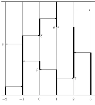
To formally construct the process and define a useful dual process, we recall the graphical representation of the biased voter model introduced by Harris (1976) and developed by Griffeath (1978). The ingredients are arrows that spread fluid in the direction of their orientation, andδ’s which are dams that stop fluid. At timessof ˜Px,y we draw an arrow from (s, y)→(s, x). At
timessofPx,ywe draw an arrow from (s, y)→(s, x) and put aδ at (s−, x). The s− indicates that the δ is placed just before the head of the arrow. Intuitively, we inject fluid into the bottom of the graphical representation at the sites of the configuration that are 1 and let it flow up. A sitex is in state 1 at timetif and only if it can be reached by fluid. If there is fluid aty
at timesand an arrow (with noδ) from (s, y)→(s, x), the fluid will spread to x, i.e., there is a birth at x if it is in state 0. If x is already occupied no change occurs.
−2 −1 0 1 2 3
✲
✲ ✛
✛
✛ ✛
✲
✛ ✲
✲
δ
δ
δ
δ
δ
Fig 1. Duality for the biased voter model.
before after
y x y x
1 0 1 1
0 1 0 0
1 1 1 1
0 0 0 0
In the first case the fluid spreads from y to x as if there was no δ. In the second, there is no fluid to be spread but the dam stops the fluid at x. In the third the dam stops the fluid at x, but it replaced by fluid from y. In the fourth, there is no fluid so nothing happens. Thus the effect in all cases is that ximitates y.
To define the dual, we inject fluid at x at time t and let it flow down. It is again stopped by dams but now moves across arrows in the direction OPPOSITE to their orientation. Givenz∈Λn= (Ln−1Z)× {1, . . . , Mn}, we
can be reached by fluid starting atz. A little thought shows thatζ0t,z ={z}
and follows the following rules:
• If a particle inζst,z is at x and an arrival inPx,y occurs at time t−s
then the particle jumps toy.
• If a particle inζst,z is at x and an arrival in ˜Px,y occurs at time t−s
then the particle gives birth to a new particle at y.
• If a jumping particle or an offspring lands on another particle in ζst,z,
then the two particles coalesce to 1.
For a picture see Figure 1. There the dark lines give the occupied sites in
ζst,1. At the end ζtt,1 ={−2,−1,1,3}.
To extend the definition to a collection of sitesA, we letζst,A=∪z∈Aζst,z.
We defined our dual process starting at a fixed timetso that the relationship in Lemma 1 holds with probability 1. If we have two times t < t′ then
the distributions of ζst,A and ζt ′,A
s agree up to time t, so the Kolmogorov
extension theorem implies that we can define a process ζsA for all time so that the distribution agrees withζst,Aup to timet. The collection of processes
{ζA: A⊂Λ
n}is referred to as the dual process of ξ.
It follows from the definition that
Lemma 1. ξt(z) = 1 for some z ∈A if and only if ξ0(x) = 1 for some x∈ζtt,A.
1.2. Measure valued limit for the biased voter model. We define the ap-proximate density by
unt(w) := 1
Mn Mn
X
i=1
ξt(w, i)
and linearly interpolate between demes to define unt(w) for all w ∈ R. We
retain the superscriptn on unt to be able to distinguish the approximating process from its limit. It is clear that for allt≥0, we have 0 ≤un
t(w) ≤1
for all w∈ Rand unt ∈Cb(R), the set of bounded continuous functions on R. If we equipCb(R) with the metric
(1) kfk=
∞
X
k=1
2−k sup
|x|≤k| f(x)|
i.e., uniform convergence on compact sets, then Cb(R) is Polish and the
pathst7→un
Theorem1. Suppose that asn→ ∞, the initial condition un0 converges in Cb(R) to f0 and that:
(a) αn≡rnMn/L2n→α∈(0,∞)
(b) βn≡Mn/Rn→β ∈[0,∞)
(c) γn≡rn/Ln→ γ∈[0,∞)
(d) Ln→ ∞ and LnRn→ ∞
Then the approximate density process (unt)t≥0 converges in distribution in D([0,∞), Cb(R)), as n→ ∞, to a continuous Cb(R) valued process (ut)t≥0
which is the weak solution to the (stochastic) partial differential equation
(2) ∂tu=α∆u+ 2θ β u(1−u) +|4γ u(1−u)|1/2W˙
with initial condition u0 = f0. Here W˙ is the space-time white noise on
[0,∞)×R.
Theorem 1 is a straight forward generalization of a result of Mueller and Tribe [38]. They considered a long range voter model onZ/n in which two
voters are neighbors if |x−y| ≤ n1/2. Their voters change their opinion at rate O(n) and imitate the opinion of a neighbor chosen at random. More precisely, for each of the 2n1/2 neighbors, they adopt the opinion of that
neighbor at rate n1/2 if it is 0 and at rate n1/2 +θn−1/2 if it is 1. Their model corresponds roughly in our situation to Ln=Mn=Rn=rn=n1/2.
Their limit is
∂tu= 1
6∆u+ 2θ u(1−u) +|4u(1−u)|
1/2W .˙
β=γ = 1 while the 1/6 comes from the fact that the variance of the uniform distribution on [−1,1] is 1/3.
Why is Theorem 1 true? If this discussion becomes confusing the reader can skip it. In Section3the analysis of the approximate martingale problem will give a more rigorous version of this explanation.
• To begin we note that only branching events change the expected number of ones. They occur from each site at rate 2θMn/Rn. Birth
events from x to y ∼ x with ξt(x) = 1 and ξt(y) = 0 will change the
local density of 1’s by 1/MnLn. In an interval of length h there are hLnMn possibilities for x, so using the assumptionMn/Rn→β gives
the drift term≈2θ β u(1−u).
so for the rest of the computation argument they can be ignored. Voting events occur from each site at rate 2rnMn. If they go from x
toy∼x withξt(x)6=ξt(y) then the local density of 1’s will change by ±1/MnLn. In an interval of lengthhthere arehLnMn possibilities for x, so using the assumptionrn/Ln→γ the infinitesimal variance term
is≈4γu(1−u).
• To see the source of the Laplacian note that in the dual particles jump at rate 2rnMnby an amount that±1/Lnwith equal probability so the
genealogies converge to Brownian motions with variance 2αt. Recalling the 1/2 in the generator of Brownian motion we have the termα∆u.
1.3. Convergence of the dual to Branching Brownian motions. Durrett and Restrepo [18] have earlier considered a related coalsescing random walk (with no births) onZ. We use their notation even though it conflicts slightly
from ours. There areM haploid individuals at each site and nearest neighbor migration (i.e., jumps±1 with equal probability) occur at rate ν. Theorem 2 in [18] states the following.
Theorem 2. Sample one individual from the colony at 0 and another one from the colony at L. Let t0 be the time at which they coalesce. IfL→
∞ and M ν/L → α ∈ (0,∞) then 2t0/(L2/ν) converges in distribution to ℓ−01(ατ)whereℓ0is the local time at 0 of a standard Brownian motion started
from1 and τ is an independent mean 1 exponential random variable.
Why is this true? Since migration occurs at rate ν, it tales time of order
L2/ν to move a distanceO(L). In this time the differencesw in the location of the two particles will visit each integer between 0 and L of order L/ν
times. If we want coalescence to have a probability strictrly between 0 and 1, we needM ν/L→α∈(0,∞).
The proof of Theorem2generalizes easily to give:
Theorem 3. Suppose that as n → ∞, the conditions on rn, Rn, Mn
and Ln in Theorem 1 hold. Then the dual process ζ of ξ converges in
dis-tribution to a limit in which particles move according to Brownian motions on the real line R with variance 2αt, branching occurs at rate θβ and two
particles coalesce when the local time at 0 of the difference between their locations exceeds ατ /γ, where τ is a mean one exponential random variable independent of the particle motions. If γ = 0 there is no coalescence.
in Theorem3, then Lemma 1and Theorem3 imply
(3) EY
x∈A
(1−ut(x)) =E Y
y∈χA t
(1−u0(y)).
Here A can be a multi-set, e.g., {a, a, a, b, b}. In this case we start three particles ataand two at b and duality says
E[(1−ut(a))3(1−ut(b))2] =E Y
y∈χA t
(1−u0(y)).
The duality relationship described in the last paragraph is not new. In 1986, Shiga and Uchiyama [43] introduced it to study a collection of Wright-Fisher diffusions coupled by migrations. Shiga [44] used it to show uniqueness in law for (2). Doering, Mueller, and Smereka [12] gave a simpler description and derivation of the dual. See also Hobson and Tribe [27].
1.4. Tracer Dynamics. Hallatschek and Nelson [25] take an interesting approach to studying the ancestral lineage of a particle. That is, the path within the dual ζsx,t that gives the actual ancestor at time t−s of the
individual atx at timet. Think of our expanding population as a fluid and inject a small amount of red liquid at time 0. The locations of the red fluid at timetwill identify the locations of their progeny. In particle terms, we will have states 0, 1, and 1∗ where the * indicates being labeled by the tracer.
ξ(x) is the indicator of the particle atxbeing in states 1 or 1∗. To construct the labeled process it is convenient to use the graphical representation. If there is an arrow-δ from y to x then x adopts the state of y. If there is an arrow fromy to x and y is in state 1 or 1∗ thenx will adopt the state ofy, but nothing happens ify is in state 0. In fluid terms, the color of fluid at y
replaces that atx.
The interacting particle system (IPS) dual process gives us the set of possible ancestors of the particle atxat time t. To analyze our new process with labeled and unlabeled particles, we assign an ordering to the particles in the IPS dual in such a way that the FIRST occupied site in the list will be the ancestor. The rules are as follows:
• If particleijumps and there is no coalescence, then its location changes but the order does not.
• If particle i jumps and coalesces with j then the particle with the higher index is removed from the dual. The surviving particle has its location updated. The remaining particles are reindexed.
To explain the definition, we will work through the example drawn in Figure
1. The successive states are
{1}, {0,1}, {0,2}, {−1,2}, {−1,3,2},
{0,−1,3,2}, {1,−1,3,2}, {1,−1,3}, {1,−2,−1,3}
To see this note that under our rules, at the point where the dual jumps from{1} → {0,1}, if there is a particle at 0 it will give birth and replace any particle at 1. The next two events involve voting, so the affected particles move but do not change their position in the ordering. The next event is an arrow from 3 to 2. A particle at 3 will replace one at 2, so 3 is inserted in the list before 2. The next novel event is the seventh transition when the particles at 2 and 1 coalesce: at that time we drop the lower ranked particle. For example, the actual ancestor of the particle (t,1) is 1 ifξ0(1) = 1; the
actual ancestor is−2 ifξ0(1) = 0 andξ0(−2) = 1.
Neuhauser [40] used a similar dual to show that in the multitype contact process, if the particle death rates are equal, then the one with the higher birth rate takes over the system. The idea of assigning an ordering to the particles to trace their genealogies is quite similar to that in the lookdown constructions of Donnelly and Kurtz [13,14]. There each particle is initially assigned a level. Genealogies of any set of particles can be read off from the evolution of the levels. See also Etheridge and Kurtz [20] for the lookdown constructions for a very general class of population models.
To do computations, we let ηt(x) = 1 if the individual at x at time t in
the biased voter model is labeled and 0 otherwise. We only label type 1’s, so ηt(x) ≤ξt(x). As noted above ηt(x) can be computed using the version
of the dual ζst,x in which the points are ordered. That is, ηt(x) = 1 if and
only if the first occupied site in the list is labeled. More formally, if under the ordering ζtt,x ={y1, y2, . . . yK} (note that K and y1, . . . yK are random
variables), then
P(ξt(x) = 0) =E K Y
i=1
(1−ξ0(yi)) !
≡EF(ζtx)
P(ηt(x) = 1) =E
K X
j=1 η0(yj)
jY−1
i=1
(1−ξ0(yi))
In the same way one computes
P(ξt(x1) = 0, . . . ξt(xm) = 0, ηt(xm+1) = 1, . . . , ηt(xn) = 1)
(4)
=E "m
Y
i=1 F(ζxi
t ) n Y
i=m+1 G(ζxi
t ) #
A standard argument shows that the probabilities just computed determine the distribution of (ξt, ηt).
As before, we define the approximate density for the labeled particles by
ℓnt(w) := 1
Mn Mn
X
i=1
ηt(w, i)
and linearly interpolate to obtain a function ℓnt(w) for all w ∈ R. The
fol-lowing is the main result of this paper.
Theorem 4. Suppose that as n → ∞, the conditions on rn, Rn, Mn
and Ln in Theorem 1 hold, and that the initial condition (un0, ℓn0) con-verges in Cb(R)×Cb(R) to(f0, g0). Then the pair of approximate densities
(un
t, ℓnt)t≥0 converges in distribution in D([0,∞), Cb(R)×Cb(R)) to a
con-tinuous Cb(R)×Cb(R) valued process (ut, ℓt)t≥0 which is the weak solution
to the coupled (stochastic) partial differential equations
∂tu=α∆u+ 2θ β u(1−u) +|4γ ℓ(1−u)|1/2W˙ 0+|4γ(u−ℓ)(1−u)|1/2W˙ 1
∂tℓ=α∆ℓ+ 2θ β ℓ(1−u) +|4γ ℓ(1−u)|1/2W˙ 0+|4γ ℓ(u−ℓ)|1/2W˙ 2
with initial condition (u0, ℓ0) = (f0, g0), where W˙ i, i = 0,1,2 are three
independent space-time white noises on[0,∞)×R.
As the proof shows the three noises ˙W0, ˙W1 and ˙W2 refer to voting
inter-actions between 1∗ and 0, 1 and 0, and 1∗ and 1 respectively. The drift inℓt
is 2θβ ℓ(1−u) because labeled particles only have a selective advantage in competition with those of type 0.
We will prove our result by showing that the sequence of approximating processes is tight. To conclude that there is weak convergence, we need to show
To do this we use our duality function (4). Details are in Section8.
In Theorems 1, 3 and 4, the assumption α > 0 is used crucially in the proof of tightness, but we allow β or γ to be 0. The deterministic regime (γ = 0) occurs, for instance, if rn=n1/a,Ln=n1/b,Mn=⌈αn2/b−1/a⌉and Rn =Mn/β, where 2a > b > a > 0. When γ = 0 the limiting process is a
PDE
∂tu=α∆u+ 2θ β u(1−u) ∂tℓ=α∆ℓ+ 2θ β ℓ(1−u).
This PDE obviously has a unique weak solution (solve the first equation and then solve the second), but if one wants, this can be proved using duality.
1.5. Lineage dynamics. Using tracer dynamics Hallatschek and Nelson [25], see page 163 and Appendix A, heuristically derived the probability density G(x, t|x′, t′) that an individual at x′ at time t′ is descended from
an ancestor at x at time t < t′. Here we describe their argument with
the hope that someone can find a way to make it rigorous. Making sense of equation (5) for the ancestral lineages seems difficult, but since these lineages are embedded in the limit of the branching coalescing random walk their behavior cannot be too pathological.
The authors of [25] considered a more general situation in which the population density in a frame moving with velocity v is
∂tu(x, t) =D∂x2u(x, t) +v∂xu(x, t) +K(x, t)
where, for instance, K(x, t) = su(1−u) +ǫpu(1−u)Z with Z being a space-time White noise, and we have changed theircto u. They concluded, see their (3), that
∂tG(x, t|x′, t′) =−∂xJ(x, t|x′, t′)
J(x, t|x′, t′) =−D∂xG+{v+ 2D∂xlog[u(x, t)]}G.
Here (x′, t′) is thought of as the initial condition and (x, t) as the finial condition, so this is the forward equation
(5) ∂tG=D∂x2G−∂x({v+ 2D∂xlog[u(x, t)]}G)
and the drift in the diffusion process isv+ 2D∂xlog[c(x, t)].
As we will now show, a closely related equation “follows” from Theorem
Suppose (u, ℓ) solves the SPDE and let ρ=ℓ/u. By Theorem 4,
∂tρ =
u ∂tℓ − ℓ ∂tu u2 =
1
u h
α∆ℓ+ 2θ β ℓ(1−u) +|4γℓ(1−u)|1/2W˙ 0
+|4γℓ(u−ℓ)|1/2W˙ 2i − ℓ u2
h
α∆u+ 2θ β u(1−u)
+|4γℓ(1−u)|1/2W˙ 0+|4γ(u−ℓ)(1−u)|1/2W˙ 1i.
The terms involving θβ cancel. To combine the Laplacian terms we use the formula
∆
ℓ u
= ∆ℓ
u − ℓ∆u
u2 −2 ∂xu
u ·∂x
ℓ u
.
To add up the noises we note that since the Wi are independent, the
vari-ances add up to
(u−ℓ)2
u4 ℓ(1−u) +
ℓ(u−ℓ)
u2 +
ℓ4(u−ℓ)(1−u) u4
=ℓ(u−ℓ)
u2
u−ℓ)(1−u)
u2 + u2 u2 +
ℓ(1−u)
u2
= ℓ(u−ℓ)
u3
since (u−ℓ)(1−u) +ℓ(1−u) +u2 =u(1−u) +u2 = u. Combining our
calculations,
(6) ∂tρ = α∆ρ+ 2α ∂xlogu·∂xρ + |4γ ρ(1−ρ)/u|1/2W˙
for some white noise ˙W. To compare (6) with (5), note that their D = α, they work in a moving reference frame and their equation is for a fixed realization of the total population size; while ours is in a fixed reference frame and does not condition on u(t, x) and hence retains the fluctuation term|4γ ρ(1−ρ)/u|1/2W˙ .
Equations (5) and (6) both contain drift terms of the form∂xlog[u(x, t)].
It is a well-known fact that solutions of the SPDE in (2) are H¨older contin-uous with exponent 1/2−ǫ in space and 1/4−ǫin time, so it is not clear how to make sense of these equations. The fact that ηt(x) ≤ ξt(x) means
thatℓ ≤u, so in computingℓ/u we will never divide a positive number by 0. However solutions touhave compact support [37], so it is not clear if the ratio of densitiesℓn/un will be tight.
for (unt, ℓnt) and formulate approximate martingale problems. This is now a common approach in the study of scaling limits of particle systems, see [17,11,16]. The calculations for theuequation are almost identical to those in Section 3 of Mueller and Tribe [38], but some minor changes are needed to study the joint distribution (ℓ, u).
In Sections 5–7 we prove tightness. Again many of the ideas come from [38], but since they only write out the details for their contact process limit theorem, and we have to prove the joint convergence, we have written out the details. See Kleim [31] for a recent example of convergence of rescaled Lotka-Volterra models to a one-dimensional SPDE, this time with a cubic drift term. The main ideas of the tightness proof are given in Section 5. Two lemmas that require a lot of computation are proved in Section 6. Some nonstandard random walk estimates are proved in Section 7. Finally Lemma2, which establishes distributional uniqueness for the coupled SPDE by using a duality based on (4), is proved in Section 8.
Acknowledgement. We would like to thank Carl Mueller and Edwin Perkins for their help while we were writing this paper. Two referees made many detailed comments that improved the readability (and correctness) of this paper.
2. Proof of Theorem 3. To get started suppose that there are no births in the dual and consider the special case in which there are initially two particles. LetStn be a random walk that jumps from x to x±1/Ln at rate 2rnMn. The reader should think of this difference of the location of two
particles (hence the factor of 2 in 2rnMn), but we allow the two lineages to
move independently even after they hit. An elementary computation shows that if
Vtn= 4rnMn
Ln Z t
0
1(Sn s=0)ds
|Stn| −Vtn is martingale. Ast→ ∞,|Stn|converges to the absolute value of a Brownian motion Bt with variance 4αt.
The next result has been proved for finite variance random walks by Borodin [4] in 1981. To keep this paper self-contained, we will give a simple proof for the nearest neighbor case.
Lemma 3. Vn
t converges in distribution to ℓ0(t) the local time at 0 for
the Brownian motion Bt.
stopping time
EVSn+t−VS ≤E0Vtn≤c
√
t
so by Aldous criterion (see e.g., Theorem 4.5 on page 320 of Jacod and Shiryaev [28] the sequenceVtnis tight. LetVtn(k)be a convergent subsequence with limitVt.|Stn(k)−V
n(k)
t is a martingale. Using the maximal inequality on
the random walk, and the dominated convergence theorem on the increasing process, both processes converge to their limits in L1. Since conditional
expectation is a contraction inL1, it follows that |Bt| −Vt is a martingale.
Now ℓ0(s) is the increasing process associated with |Bt| See e.g., (11.2) on
page 84 of Durrett’s Stochastic Calculus book [15]. By the uniqueness of the Doob- Meyer decomposition, there is only one subsequential limit, so the entire sequence converges in distribution toℓ0(t).
The sojurn times at 0 are independent and exponential with rate 4rnMn,
so the number of visits to 0 up to timet
Ntn∼4rnMn Z t
0
1(Sn s=0)ds
and it follows that Ntn/Ln → ℓ0(t). On each visit to 0, the two particles
have a probability 1/Mn to coalesce. Our assumptions imply that
Mn Ln ·
rn Ln →
α so Ln
Mn → γ α
and the desired result has been proved for the processes with no births. To add births we note there areMn cells at each deme and ˜Pxy has rate θR−n1,
so the branching rate at each deme isθMnR−n1 →θβ.
3. Approximate Martingale Problems. For simplicity we drop the subscriptn’s onM,L,Rand r. We leave the superscriptninunt and ℓnt to distinguish the approximating processes from their limits. We write
hf, gi:= 1
L X
w∈L−1Z
f(w)g(w)
whenever h|f|,|g|i <∞ and adopt the convention that φ(x) :=φ(w) when
3.1. Type 1 particles. To develop the martingale problem, we note that dynamics of (ξt)t≥0 can be described by the equation
ξt(x) =ξ0(x) + X
y∼x Z t
0
(ξs−(y)−ξs−(x))dPsx,y
(7)
+X
y∼x Z t
0
ξs−(y)(1−ξs−(x))dP˜sx,y.
In the first integral, ifξs−(y) =ξs−(x) then nothing happens.
Ifξs−(y) = 1 andξs−(x) = 0 thenξs(x) = 1;
if ξs−(y) = 0 andξs−(x) = 1 then ξs(x) = 0.
In the second integral, nothing happens unlessξs−(y) = 1 and ξs−(x) = 0.
In this case ξs(x) = 1.
Letφ: [0,∞)×R→Rbe continuously differentiable in t, twice
continu-ously differentiable inx and have compact support in [0, T]×R for anyT. Applying integration by parts toξt(x)φt(x), using (7), and summing overx,
we obtain for allt∈[0.T],
hunt, φti−hun0, φ0i − Z t
0 h
uns, ∂sφsids
= (M L)−1X
x X
y∼x Z t
0
(ξs−(y)−ξs−(x))φs(x)dPsx,y
(8)
+ (M L)−1X
x X
y∼x Z t
0
ξs−(y)(1−ξs−(x))φs(x)dP˜sx,y.
(9)
Drift term. We break (9) into an average term and a fluctuation term (M L)−1X
x X
y∼x Z t
0
ξs−(y)(1−ξs−(x))φs(x)θR−1ds
(10)
+ (M L)−1X
x X
y∼x Z t
0
ξs−(y)(1−ξs−(x))φs(x) (dP˜sx,y−θR−1ds).
(11)
Recalling the definition of the density, (10) becomes
θ·M R ·
1
L X
w∈L−1Z Z t
0
SinceM/R→β, this converges to
θβ Z t
0 Z
R
2us(w)(1−us(w))φs(w)dw ds
asn→ ∞. Here, and in what follows, the claimed convergences follow once we have provedC-tightness (see Section 5 for the proof). We have established convergence of finite dimensional distributions so the sequences of processes converge in distribution.
The second term (11) is a martingale Et(2)(φ) with
hE(2)(φ)it≤ θ R(M L)2
X
x X
y∼x Z t
0
φ2s(x)ds
≤LR2θ
Z t
0 h
1, φ2sids→0 sinceLR→ ∞.
White noises. We can rewrite (8) as (12) (M L)−1X
x X
y∼x Z t
0 {
ξs−(y)[1−ξs−(x)]−ξs−(x)[1−ξs−(y)]}φs(x)dPsx,y.
We now rewrite the integrand as
ξs−(y)[1−ξs−(x)]φs(y)−ξs−(x)[1−ξs−(y)]φs(x)
(13)
+ξs−(y)[1−ξs−(x)](φs(x)−φs(y)).
(14)
We work first with (13). Interchanging the roles of x and y in the double sum, letting ξtc(z) = 1−ξt(z), and writing Qx,yt = Psy,x−Psx,y this part of
(12) becomes
(15) (M L)−1X
x X
y∼x Z t
0
ξsc−(y)ξs−(x)φs(x)dQx,yt .
To prepare for treating the joint SPDE we split (15) into Z0
t(φ) +Zt1(φ)
where theZti(φ) are defined by the next two equations
(M L)−1X
x X
y∼x Z t
0
ξsc−(y)ηs−(x)φs(x)dQy,xs ,
(16)
(M L)−1X
x X
y∼x Z t
0
ξsc−(y) (ξs−(x)−ηs−(x))φs(x)dQy,xs .
These two martingale terms use the same Poisson processes but the product of their integrands is 0 since (1−ξt(x))ηt(x) vanishes for allxand t. Hence
these martingales are uncorrelated.
The variance process hQx,yit = 2rt. Our assumptions on φ imply that
sups∈[0,t]|φs(x)−φs(y)| ≤Kt/Lfor someKt<∞, so ignoring the difference
betweenφs(x) and φs(y), we have
hZ0(φ)it= 4rL−2 Z t
0 X
w∈L−1Z
ℓns−(w)(1−uns−(w))φs(w)2ds+o(1)
which converges to
4γ Z t
0 Z
R
ℓs(w)(1−us(w))φs(w)2dw ds sincer/L→γ.
Similarly, hZ1(φ)it converges to
4γ Z t
0 Z
R
(us(w)−ℓs(w)) (1−us(w))φs(w)2dw ds.
Laplacian Term. We denote the discrete gradient and the discrete Laplacian respectively by
∇Lf(w) :=L
f(w+L−1)−f(w) (18)
∆Lf(w) :=L2
f(w+L−1) +f(w−L−1)−2f(w).
(19)
We break (14) into an average term and a fluctuation term
(M L)−1X
x X
y∼x Z t
0
ξs−(y)ξsc−(x)[φs(x)−φs(y)]r ds
(20)
+ (M L)−1X
x X
y∼x Z t
0
ξs−(y)ξcs−(x)[φs(y)−φs(x)](dPsx,y−r ds).
(21)
We can replace ξsc− by 1 in (20) without changing its value, because by symmetry,PxPy∼xξs−(y)ξs−(x)[φs(x)−φs(y)] = 0 for alls >0.
Doing the double sum overy and then over x∼y the above is
rM L2 ·
1
L X
w
uns−(w)∆Lφs(w) = rM
L2 hu n
By assumption rM/L2 → α, so this term converges to αRRus∆φs. The
other term, (21), is a martingaleEt(1)(φ) with
hE(1)(φ)it≤ r
(M L)2 X
x X
y∼x Z t
0
(φs(x)−φs(y))2ds
(22)
= 2r
L3 Z t
0 h
1,|∇Lφs|2ids→0
(23)
sincer/L→γ and L→ ∞.
Combining our calculations, we see that in the limitn→ ∞,
Z
R
ut(w)φt(w)dw −u0(w)φ0(w)dw− Z t
0 Z
R
us(w)∂sφs(w)dw ds
−
Z t
0 Z
R
αus(w)∆φs(w)−2θβ us(w)(1−us(w))φs(w)dw ds
(24)
is a martingale with quadratic variation
(25) 4γ
Z t
0 Z
R
us(w)(1−us(w))φ2s(w)dw ds
which is the martingale problem formulation of (2).
3.2. Labeled Particles. To begin, we note that in terms of the previously defined Poisson processes,
ηt(x)−η0(x) = X
y∼x Z t
0
(ηs−(y)−ηs−(x))dPsx,y
(26)
+X
y∼x Z t
0
ηs−(y)(1−ηs−(x))−ξs−(y)(1−ηs−(y))ηs−(x)dP˜sx,y.
The first term gives the voter interactions. For the second term, note that ify is in state 1∗ andxis not, the number of 1∗’s will increase by 1, while if
xis in state 1∗ and y is in state 1 (ξ
s−(y) = 1 andηs−(y) = 0), the number
will decrease by 1.
Arguing as for the type 1 particles while using (26) instead of (7), we get
hℓnt, φti − hℓn0, φ0i − Z t
0 h
ℓns, ∂sφsi
= (M L)−1X
x X
y∼x Z t
0
(ηs−(y)−ηs−(x))φs(x)dPsx,y
(27)
+ (M L)−1X
x X
y∼x Z t
0
[ηs−(y)−ξs−(y)ηs−(x)]φs(x)dP˜sx,y,
where we have simplified the second term of (26) using ξs−(y)ηs−(y) =
ηs−(y).
Drift term. Breaking the second term (28) into an average term and a fluctuation term as before, we conclude that asn→ ∞, the average term is
θM LR
X
w∈L−1Z Z t
0
ℓns(w+L−1)−usn(w+L−1)ℓns(w)
+ℓns(w−L−1)−uns(w−L−1)ℓns(w)φs(w)ds
which converges to
θβ Z t
0 Z
R
2ℓs(w)(1−us(w))φs(w)dw ds.
White noises. We again change the integrand in (27) to {ηs−(y)[1−ηs−(x)]−ηs−(x)[1−ηs−(y)]}φs(x)
and then split it into two parts as in (13) and (14). That is, we rewrite the integrand as
ηs−(y)[1−ηs−(x)]ηs(y)−ηs−(x)[1−ηs−(y)]φs(x)
(29)
+ηs−(y)[1−ηs−(x)](φs(x)−φs(y)).
(30)
Arguing as before, we obtain the following sum coming from (29).
(M L)−1X
x X
y∼x Z t
0
[1−ξs−(y)]ηs−(x)φs(x) (dPsy,x−dPsx,y)
(31)
+(M L)−1X
x X
y∼x Z t
0
[ξs−(y)−ηs−(y)]ηs−(x)φs(x) (dPsy,x−dPsx,y).
The first noise is the same asZ0
t(φ) in (16) while the second noise, denoted
by Zt2(φ), has variance converging to
4γ Z t
0 Z
R
ℓs(w) (us(w)−ℓs(w))φs(w)2dw ds.
The product of any two of the three integrands inZti(φ) (i= 0,1,2) is 0, so these three martingales are uncorrelated.
Laplacian term. Breaking (30) into an average term and a fluctuation term as was done for (14), we see that as n→ ∞, the average term
rM L2 hℓ
n
s−,∆Lφsi →α Z
R
Combining our calculations, we see that in the limit, for any φ, ψ ∈ Cc1,2([0,∞)×R),
Z
R
(utφt−u0φ0+ℓtψt−ℓ0ψ0)dw
−α Z t
0 Z
R
us(∂sφs+ ∆φs) +ℓs(∂sψs+ ∆ψs)dw ds
−2θ β Z t
0 Z
R
us(1−us)φs + ℓs(1−us)ψsdw ds
(32)
is a continuous martingale with quadratic variation
(33) 4γ Z t
0 Z
R
us(1−us)φ2s+ℓs(1−ℓs)ψs2 + 2φsψsℓs(1−us)dw ds.
Any sub-sequential limit (u, ℓ) solves this martingale problem. It is standard (see p. 536-537 in [38]) to show that (u, ℓ) then solves the coupled SPDE in Theorem4weakly, with respect to some white noises.
4. Green’s function representation. As remarked earlier our proof follows the approach in [38]. The first step is to prove the analogue of their (2.11). Observe thatunt(z) =hunt, L1zi and ℓnt(z) =hℓnt, L1zi, where 1z is
the function onL−1Zwhich is 1 atzand zero elsewhere. Letαn=rnMnL−n2
which converges toα asn→ ∞ and let
(34) pnt(w) :=LP(Xn
t =w|X0n= 0)
be the transition probability of the simple random walk (Xt(n))t≥0 on L−1Z
with jump rate 2L2, so that it converges to pt(w) the transition density of
Brownian motion run at rate 2. Let {Pn
t }t≥0 be the associated semigroup
which has generator the discrete Laplacian ∆L defined in (19).
Applying the approximate martingale problems with test function
(35) φs(w) :=φt,zs (w) := (
pn
αn(t−s)(w−z) for s∈[0, t],
0 otherwise
and using the facts that ∂sφs+αn∆Lφs= 0 and hun0, φt,z0 i=Pαnntu
n 0(z), we
have
fort≥0 andz∈L−1Z. HereZt(φ),E(1)
t (φ) andE (2)
t (φ) are martingales
de-fined in (15), (21) and (11) respectively, withφsdefined in (35). To describe
the other term, we letβn=M R−1 which converges toβ, and let Yt(φ) be
(37) θβn
L Z t
0 X
w∈L−1Z
[uns(w−L−1) +uns(w+L−1)](1−uns(w))φs(w)ds.
Repeating the last argument for the labeled particles,
(38) ℓnt(z) =Pαnntℓn0(z) +Ytℓ(φ) +Ztℓ(φ) +Etℓ,1(φ) +Etℓ,2(φ).
Here Zt(ℓ)(φ) := Z0
t(φ) +Zt2(φ) is given by (31), E (ℓ,2)
t (φ) is obtained by
replacing (ξ, ξc) by (η, ηc) in (21), Et(ℓ,2)(φ) is the fluctuation term corre-sponding to (28). The remaining term is
Ytℓ(φ) = θβn
L Z t
0 X
w∈L−1Z h
ℓns(w+L−1)−usn(w+L−1)ℓns(w)
+ℓns(w−L−1)−uns(w−L−1)ℓns(w)iφs(w)ds.
5. Tightness. Recall that a sequence of probability measures is said to beC-tight, if it is tight in Dand any subsequential limit has a continuous version. The goal of this section is to prove:
Theorem 5. Suppose the assumptions in Theorem 1 hold. Then the sequence{(un, ℓn)}n≥1 isC-tight inD([0, T], Cb(R)×Cb(R))for everyT >
0.
Proof. The compact containment condition (condition (a) of Theorem 7.2 in [21, Chapter 3]) holds trivially as 0≤ℓn≤un≤1. SinceCb(R)×Cb(R)
is equipped with the product metric, the desired C-tightness follows once we can show that for anyǫ >0, one has
lim
δ→0lim supn→∞ P
sup
t1−t2<δ 0≤t2≤t1≤T
unt1 −unt2 > ǫ
= 0,
(39)
lim
δ→0lim supn→∞ P
sup
t1−t2<δ 0≤t2≤t1≤T
ℓnt1−ℓnt2 > ǫ
= 0.
(40)
First term in(36) and (38). By standard coupling arguments for simple random walk, we can check as in Lemma 7(b) of [38] that, upon linearly interpolatingPαnntun0(z) in space, we have
(41) sup
t∈[0,T]k
Pαnntun0 −Pαntf0k →0 asn→ ∞,
where{Pt}t≥0is the semigroup for the Brownian motion inRrunning at rate
2, andf0 is the initial condition foru functions in Theorem4. This implies,
by the continuity of the semigroup Pt, that (39) holds with unt replaced by Pαnntun0. By the same reasoning, we have
(42) sup
t∈[0,T]k
Pαnntℓn0 −Pαntg0k →0 asn→ ∞
whereg0 is the initial condition for ℓfunctions in Theorem 4.
Remaining terms in (36) and (38). For simplicity, we write
b
unt(z) :=Yt(φ) +Zt(φ) +Et(1)(φ) +E (2) t (φ), b
ℓtn(z) :=Yt(ℓ)(φ) +Zt(ℓ)(φ) +Et(ℓ,1)(φ) +Et(ℓ,2)(φ).
The next moment estimate for space and time increments is similar to Lemma 6 in [38], but ours implies H¨older continuity of the limits with ex-ponent<1/2 in space and<1/4 in time.
Lemma4. For anyp≥2andT ≥0, there exists a constantC(T, p)>0 such that
E|ubnt1(z1)−ubnt2(z2)|p ≤CT,p
|t1−t2|p/4+|z1−z2|p/2+M−p
(43)
E|ℓbnt1(z1)−ℓbnt2(z2)|p ≤CT,p|t1−t2|p/4+|z1−z2|p/2+M−p
(44)
for all0≤t2 ≤t1 ≤T, z1, z2 ∈L−1Z and n≥1.
The proof of this result is postponed to the next section since it requires a number of computations. We now argue that (43) implies (39) holds forubn. This idea is described in the paragraph before Lemma 7 in [38] and page 648 of [31]: we approximate the c`adl`ag processbunby acontinuousprocess ˜uand invoke a tightness criterion inspired by Kolmogorov’s continuity theorem.
andlimn→∞θn= 0. Then there existsn0 ∈Nsuch that for anyp≥2,T ≥0
andK ≥0,
(45) E|u˜nt1(z1)−u˜nt2(z2)|p ≤CT,p,K
|t1−t2|p/4+|z1−z2|p/2
,
for all0≤t2 ≤t1 ≤T, zi ∈R with |zi| ≤K (i= 1,2) and n≥n0.
By a standard argument (see, for example, Problems 2.2.9 and 2.4.11 of [29]), one can show that (45) implies that (39) holds whenu is replaced by ˜
un. Finally, by the reasoning in the proof of Lemma 7(a) in [38], there is a σ >0 so that
lim sup
n→∞
P sup
t∈[0,T]k
˜
unt −buntk ≥n−σ = 0.
Therefore (39) holds for ubn. By the same argument, (44) implies (40) holds forbℓn. Theorem5 will be proved once Lemmas4 and 5 are.
6. Proofs of Lemmas 4 and 5.
Proof of Lemma 4. We prove only (43) for unlabeled particles. The proof of (44) for labeled particles is similar. The basic ingredients are the following estimates of time and space increments of the transition probability of simple random walk. Namely, there exists a constant C >0 independent of nsuch that
0 ≤
Z T
0
pns(0)ds≤C√T ,
(46)
0 ≤
Z ∞
0
pns(0)−pns+θ(0)ds≤C√θ,
(47)
0 ≤
Z ∞
0
pns(0)−pns(z)ds≤C|z|
(48)
Z T
0
1
L X
w
|pns+θ(w)−pns(w)|ds ≤ C√T θ,
(49)
Z T
0
1
L X
w
|pns(w)−pns(z+w)|ds ≤ C√T|z|
(50)
for θ ≥ 0, z ∈ L−1Z and T > 0. These estimates can be either found or
We will show that each of the four terms of bun satisfies (43). To simplify notation, we assume, without loss of generality for the proof, that αn ≡1.
First, we deal with the processY that has no jumps. To reduce the size of the formulas we let
vsn(w) = [usn(w−L−1) +uns(w+L−1)](1−uns(w)).
Using the definitions of Y (37) and of our test function (35) we have for
t1> t2
Yt1(φt1,z1)−Yt2(φt2,z2) =θβn Z t1
t2
1
L X
w
vsn(w)pnt1−s(z1−w)ds
+θβn Z t2
0
1
L X
w
vsn(w)[pnt1−s(z1−w)−pnt2−s(z2−w)]ds
≡θβn(Θ1(Y) + Θ2(Y)).
The sums are over w∈L−1Z, which we have omitted to simplify notation.
Since 0≤un≤1 and L−1Pwpnt(z−w) = 1 (recall the definition ofpn in (34)), we have
(51) E|Θ1(Y)|p ≤2p(t1−t2)p.
by H¨older’s inequality.
By the triangle inequality and the translation invariance and symmetry of the transition density, we obtain
Z t2
0
1
L X
w
|pnt1−s(z1−w)−pnt2−s(z2−w)|ds
≤
Z t2
0
1
L X
w
|pnt1−s(z1−z2+w)−pnt1−s(w)|+|pnt1−s(w)−pnt2−s(w)|
ds
≤CT|z1−z2|+C√t1−t2
by (50) and (49). Since 0≤vn≤2,
(52) E|Θ2(Y)|p≤CT,p √t1−t2+|z1−z2|p
for all 0≤t2 ≤t1 ≤T,z1, z2 ∈L−1Z and n≥1.
It remains to consider Et(1)(φ), Et(2)(φ) and Zt(φ). Note that for each of
them, the largest possible jump is bounded almost surely by
2(M L)−1sup
s≥0k
becauseφs, as defined in (35), is bounded byL.
We shall employ a version of the Burkholder-Davis-Gundy inequality stated at the bottom of page 527 in [38]. Namely, for any c`adl`ag martin-galeX withX0 = 0 and for p≥2,
(53) E[ sup
s∈[0,t]|
Xs|p]≤C(p)E h
hXip/t 2+ sup
s∈[0,t]|
Xs−Xs−|p
i
, t≥0.
Writing Nsx,y for the compensated Poisson process Psx,y−rns, andPx,y∼x
for the double sumPxPy∼x, we decompose
Et1(1)(φt1,z1)−Et2(1)(φt2,z2)
= 1
M L X
x,y∼x Z t1
t2
ξs−(y)ξcs−(x) pnt1−s(z1−y)−pnt1−s(z1−x)dNsx,y
+ 1
M L X
x,y∼x Z t2
0
ξs−(y)ξsc−(x) pnt1−s(z1−y)−pt1n−s(z1−x)
−pnt2−s(z2−y) +pnt2−s(z2−x)dNsx,y
≡Θ1(E(1)) + Θ2(E(1)).
Writing ˜Nsx,y for the compensated Poisson process ˜Psx,y−θR−n1swe have
Et1(2)(φt1,z1)−Et2(2)(φt2,z2)
= 1
M L X
x,y∼x Z t1
t2
ξs−(y)(1−ξs−(x))pnt1−s(z1−x)dN˜sx,y
+ 1
M L X
x,y∼x Z t2
0
ξs−(y)(1−ξs−(x))[pnt1−s(z1−x)−pnt2−s(z2−x)]dN˜sx,y
≡Θ1(E(2)) + Θ2(E(2)).
Finally, writingQx,ys =Nsy,x−Nsx,y we have
Zt1(φt1,z1)−Zt2(φt2,z2)
= 1
M L X
x,y∼x Z t1
t2
(1−ξs−(y))ξs−(x)pnt1−s(z1−x)dQx,ys
+ 1
M L X
x,y∼x Z t2
0
(1−ξs−(y))ξs−(x)[pnt1−s(z1−x)−pnt2−s(z2−x)]dQx,ys
Once we use 0≤ ξ ≤ 1 to simplify the integrands the three expressions have a similar structure. E(1) will be the smallest since it has a difference
of transition densities at adjacent sites, so we begin by estimating E(2). To estimate Θ1(E(2)), we let
Xt1 = 1
M L X
x,y∼x Z t
0
ξs−(y)ξcs−(x)pnt1−t2−s(z1−x)dN˜sx,y.
By Markov property of (ξt)t≥0 and the stationarity of the compensated
Pois-son process,
E(|Θ1(E(2))|p) =E Eξt2(|Xt1
−t2|p),
whereEξt2 is the expectation w.r.t. the law of ξ starting at ξt2.
To prepare for the next calculation we note that using the symmetry of the transition density and the Chapman-Kolmogorov equation
(54) L−1X w
[pnu(w)]2 =L−1X w
pnu(w)pnu(−w) =p2u(0).
The predictable bracket process ofX1 is
hX1it= θ
Rn(M L)2 X
x,y∼x Z t
0
ξs−(y)ξcs−(x)[pnt1−t2−s(z1−x)]2ds.
Since there are 2M values of y for each x and M values of x for each
w∈L−1Z, if we let cn= 2θ/RnLn then the above is
≤cn Z t
0
L−1X w
pnt1−t2−s(w)2ds
=cn Z t
0
pn2(t1−t2−s)(0)ds≤cnC(t1−t2)1/2
for t∈ [0, t1−t2], where in the second step we have used the (54) and in
the last step we used (46), Note thatcn→0 since RnLn→ ∞.
If we do the calculation forZ then cn= 2rn/L→2γ so we get the same
upper bound. InE(1),c
n=rn/Ln →γbut we havepnt1−s(z1−y)−pnt1−s(z1− x) instead of a singlep, so
L−1X w
pnt1−t2−s(w)−pt1n−t2−s(w−L−1)2
If we use (50) now we would get an upper bound ofCTL−1when we integrate
the above expression with respect to dsfrom s= 0 to s=T. Therefore, by (53), we have
(55) E(|Θ1|p)≤Cp(|t1−t2|p/4+M−p).
forE(1),E(2) and Z.
Similarly,E(|Θ2(E(2))|p) =E(|X2
t2|p), where
Xt2 = 1
M L X
x,y∼x Z t
0
ξs−(y)ξcs−(x)[pnt1−s(z1−x)−pnt2−s(z2−x)]dN˜sx,y
is a c`adl`ag martingale for t≤t2 with predictable bracket process
hX2it≤cn Z t
0
L−1X w
[pnt1−s(z1−w)−pnt2−s(z2−w)]2.
Arguing as before using (54) we get
≤cn Z t
0
pn2(t1−s)(0) +pn2(t2−s)(0)−2pnt2+t1−2s(z1−z2)
a result that also holds forE(1)andZ. Adding and subtracting 2pn
t2+t1−2s(0)
and using (47) and (48) the above is at most
C√t1−t2+CT|z1−z2|).
Using (53) now, we have
(56) E(|Θ2|p)≤Cp,T(|t1−t2|p/4+|z1−z2|p/2+M−p)
which holds forE(1),E(2) and Z and the proof is complete.
Proof of Lemma 5. It suffices to consider the case|t1−t2|1/4 ≤M−1
and |z1−z2|1/2 ≤M−1, since otherwise Lemma 4 easily implies (45). The
triangle inequality gives
(57) |u˜nt1(z1)−u˜nt2(z2)| ≤ |u˜nt1(z1)−u˜nt2(z1)|+|u˜nt2(z1)−u˜nt2(z2)|.
We first estimate the time difference on the right. Writesk:=kθnfork∈Z+.
Since |t1−t2| ≤M−4 < θn, we have either sk ≤t2 < t1 ≤sk+1 for some k
or t2 < sk < t1 for somek. Since ˜un is linear between grid points, in either
case
|u˜nt1(z)−u˜nt2(z)| ≤2|bunsk+1(z)−busnk(z)| ∨ |bunsk(z)−ubnsk−1(z)||t1−t2|
Hence Lemma4, the assumptionM−4 < θn and|t1−t2| ≤M−4 imply that
E|u˜n
t1(z)−u˜nt2(z)|p ≤CT,p |
t1−t2|p θnp
θp/n4+M−p
≤CT,p
|t1−t2|
θ3n/4 p
≤CT,p|t1−t2|p/4.
Next, we estimate the space difference on the right of (57). Take n large so that M−1 <(1 +γ)L−1 and (1 +γ)2L−2 < L−1 (this is possible by our assumptions on scalings, even ifγ = 0). Then|z1−z2|<(1 +γ)2L−2 < L−1.
By almost the same argument used above, we easily obtain
E|u˜nt(z1)−u˜nt(z2)|p ≤C(T, p)|z1−z2|pLp L−p/2+M−p
≤C(T, p)|z1−z2|p(Lp/2+ (1 +γ)p)
≤C(T, p)h(1 +γ)p/2|z1−z2|3p/4+ (1 +γ)p|z1−z2|p i
.
The proof of Lemma5 is complete.
7. Random walk estimates. The first two, (46) and (47), follow di-rectly from the local central limit theorem (LCLT) (see, for example, Propo-sition 2.5.6 in [35]). (49) follows from (50) and the Chapman-Kolmogorov equation: the integrand can be written as
pns+θ(w)−pns(w) = 1
L X
z∈L−1Z
pnθ(z) pns(w−z)−pns(w).
It remains to prove (48) and (50). By scaling, pn
t(w) = L pL2t(Lw) where pt(k) is the transition density of
the simple random walk onZ. The integral of (48) is therefore
1
L Z ∞
0
pns(0)−pns(Lz)ds.
Splitting this integral into two parts according to whether s≤L|z|2 or s > L|z|2, the first part is bounded by L−1R0L|z|2pns(0)ds≤C|z|/√Laccording to (46). The second part is bounded by C|z| by the LCLT.
Formula (50) is similar to Proposition 2.4.1 in [35] which says that
(58) X
k∈Z
qm(k)−qm(k+j) ≤ √C j
where qm(k) is the transition density for the discrete time simple random
walk onZ. Hence, by using scaling and an independent Poisson process Nt,
we rewrite the left hand side of (50) as
1
L2 Z L2T
0
X
k∈Z
|pns(k)−pns(k+Lz)|ds
= 1
L2 Z L2T
0
X
k∈Z
∞
X
m=0
P(Ns=m) qm(k)−qm(k+Lz)ds
which is at most
C|z| L
Z L2 T
0
∞
X
m=0
P(Ns=m)
√
m ds
by (58). Arguing as in the proof of Proposition 2.5.6 in [35] by using Propo-sition 2.5.5 (the LCLT for Poisson processes), we obtain that the integral is of order√L2T and hence (50) holds.
8. Proof of Lemma 2. To prepare for the proof for the SPDE, we begin by considering the diffusion process
(59) dU =βU(1−U)dt+σpU(1−U)dB.
Following the approach of Doering, Mueller and Smereka [12], we change variables Z= 1−U to get (recall dZ=−dU)
(60) dZ=−βZ(1−Z)dt−σpZ(1−Z)dB.
The minus in front of the diffusion term is not important here but it will be in the next calculation in (63). Using Itˆo’s formula and ignoring the martingale terms
drift(Zm) =mZm−1(−βZ(1−Z)) +m(m−1)Zm−2σ 2
2 Z(1−Z)
=βm[Zm+1−Zm] +σ
2m(m−1)
2 [Z
m−1−Zm]).
LetN(t) be a Markov process with Qmatrix
Qm,m+1 =βm Qm,m−1 =σ2
m(m−1) 2
Qm,m=−βm−σ2
Combining our calculations,
d dtEZ
m =X
n
Qm,nEZn
Letting Pℓ,m(t) = P(N(t) = m|N(0) = ℓ) be the transition probabilities,
we have
Lemma 6. For fixed T >0 and ℓ≥1, Mt=Pm∞=1Pℓ,m(T −t)Zm(t) is
a martingale.
Proof. Differentiating we have
d
dtEMt= X
m
EZm(t)d
dtPℓ,m(T−t) +Pℓ,m(T −t) d dtEZ
m(t)
=X
m
−EZm(t)X
n
Pℓ,n(T −t)Qn,m
+Pℓ,m(T−t) X
n
Qm,nEZn(t) = 0
if we interchange the roles ofm and nin the second sum.
From Lemma6 we get
(62) EZN(0)(T) =EZN(T)(0).
Now consider the system
dZ=−βZ(1−Z)dt−σ√V Z dB0−σpZ(1−Z−V)dB1,
(63)
dV =βV Z dt+σ√V Z dB0+σpV(1−V −Z)dB2,
where the Bi are independent Brownian motions. To get our second dual
function, we consider Yn= Pnm=1Zm−1V. Using Itˆo’s formula and for the
second term recall (60),
drift
n X
m=1
Zm−1V !
=V n X
m=2
(m−1)Zm−2(−βZ(1−Z))
+σ
2
2 V
n X
m=3
(m−1)(m−2)Zm−3Z(1−Z)
+
n X
m=1
Zm−1βZV −σ2 n X
m=2
where the last term comes from the fact that the covariance of Z and V is −σ2V Z. Collecting the terms with β, and changing variables k=m−1 in
the second sum we get
=βV " n
X
m=2
(m−1)Zm− n−1 X
k=1 kZk+
n X m=1 Zm # .
Adding the third sum to the first
=βV " n
X
m=1
mZm− n−1 X
k=1 kZk
#
=nβV Zn=nβ n+1 X
m=1
Zm−1V − n X
m=1
Zm−1V !
which corresponds to jumps fromnton+ 1 at rateβn. Collecting the terms withσ2 and changing variables to haveZk−1, we get
=σ2V "n−1
X
k=2
k(k−1)
2 Z
k−1− n X
k=3
(k−1)(k−2)
2 Z
k−1− n X
k=2
(k−1)Zk−1 #
.
Moving termsk= 2 ton−1 from the last sum into the first one
=σ2V "n−1
X
k=2
(k−2)(k−1)
2 Z
k−1
−
n X
k=3
(k−1)(k−2)
2 Z
k−1
−(n−1)Zn−1 #
.
Thek= 2 term in the first sum vanishes. Terms 3 ton−1 in the first sum cancel with the second sum leaving
=−σ2Vn(n−1)
2 Z
n−1=σ2n(n−1)
2
n−1 X
m=1
Zm−1V − n X
m=1
Zm−1V !
which corresponds to jumpsnto n−1 at rateσ2n(n−1)/2.
Combining our calculations
d
dtEYn= X
m
Qm,nEYn.
whereQm,n is given in (61). Using Lemma6 again,
E N(0) X m=1
Zm−1(T)V(T)
=E
N(T) X
m=1
Zm−1(0)V(0)
8.1. Duality for the Wright-Fisher SPDE. We begin by proving the du-ality result for the equation for single SPDE (2). This is a known result due to Shiga [44]. However, he did not give many details and we need to general-ize his result to our coupled SPDE, so we will follow the approach of Athreya and Tribe [1]. Letz= 1−u. Define ¯zt(x) =R zt(y)pǫ(y−x)dy wherepǫis the
normal density with mean 0 and varianceǫ. Noting thatx→zt¯(x) is smooth and using the weak formulation of (2) with test functionφǫ,x(y) =pǫ(y−x), we have
¯
zt(x)−z¯0(x) = Z t
0
α∆¯zs(x)ds
−θβ Z t
0 Z
2zs(y)(1−zs(y))pǫ(y−x)dy ds
(64)
+
Z t
0 Z p
4γzs(y)(1−zs(y))pǫ(y−x)dW.
Using Itˆo’s formula (each ¯zt(x) is a semi-martingale so this is legitimate)
and writingLz for the generator of (¯zt(x1), . . . ,z¯(xn)) withx1, . . . xn fixed,
we see that (ignoring the martingale terms)
drift Lz¯ Y
i
¯
zt(xi) !
=
n X
i=1 Y
j6=i
¯
zt(xj)α∆¯zt(xi)
+ 2θβ n X
i=1 Y
j6=i
¯
zt(xj) Z
[zt2(y)−zt(y)]pǫ(y−xi)dy
(65)
+ 4γ n−1 X
i=1 n X
j=i+1 Y
k6=i,j
¯
zt(xk) Z
[zt(y)(1−zt(y))]pǫ(y−xi)pǫ(y−xj)dy.
The dual process is a system of branching coalescing Brownian particles. During their lifetime the particles are Brownian motions run at rate 2α
xj−xi at 0. Writing Lx for the generator, we have
drift Lx Y
i
¯
zt(xi) !
=
n X
i=1 Y
j6=i
¯
zt(xj)α∆¯zt(xi)
+ 2θβ n X
i=1 Y
j6=i
¯
zt(xj)·[¯zt2(xi)−z¯t(xi)]
(66)
+ 4γ n−1 X
i=1 n X
j=i+1 Y
k6=i,j
¯
zt(xk)·[¯zt(xi)(1−z¯t(xj))]δ{xj=xi}
in which we used the formal notation dLi,jt = δ{xj(t)=xi(t)}dt. The precise meaning of the last term involves integration w.r.t. local times and is ex-plained in (70).
We now follow Proposition 1 in [1] to use the duality method encapsulated in Theorem 4.4.11 of Ethier and Kurtz [21]. In their notation α=β = 0.
F(¯z, x) =
n Y
i=1
¯
z(xi) if x= (x1,· · · , xn).
They supposeF(¯zt, x)−R0tG(¯zs, x)ds and F(¯z, x(t))−R0tH(¯z, x(s))ds are
martingales and conclude that for t≥0,
(67) EF(¯zt, x(0))−EF(¯z0, x(t)) =E
Z t
0
G(¯zt−s, x(s))−H(¯zt−s, x(s))ds.
In our situation, (67) holds withG(¯z, x) =L¯zF(¯z, x) andH(¯z, x) =LxF(¯z, x).
By the continuity of x 7→ zt(x), we have F(¯zt, x(0)) → F(zt, x(0)) and F(¯z0, x(t)) → F(z0, x(t)) a.s. as ǫ→ 0, so using the bounded convergence
theorem,
EF(¯zt, x(0))−EF(¯z0, x(t))→EF(zt, x(0))−EF(z0, x(t)).
To prove the desired duality formula
(68) E
n(0) Y
i=1
zt(xi(0)) =E n(t) Y
i=1
z0(xi(t)), t≥0,
it remains to argue that the RHS of (67) tends to zero asǫ→0.
The first term in (65) agrees with that of (66). For the second terms, omitting 2θβ, the integrand of the difference is
(69)
E
Z t
0 n(s) X
i=1 Y
j6=i
¯
zt−s(xj(s)) h Z
a.s. for s ∈ (0, t), by continuity of y 7→ zs(y) and dominated convergence.
The contribution to (67) from the third term of (66) is (omitting 4γ)
(70) E
Z t
0 n(Xs)−1
i=1 n(s) X
j=i+1 Y
k6=i,j
¯
zt−s(xk(s))·[¯zt−s(xi(s)) 1−z¯t−s(xj(s))]dLi,js
which converges, by dominated convergence to
(71) E
Z t
0 n(Xs)−1
i=1 n(s) X
j=i+1 Y
k6=i,j
zt−s(xk(s))·[zt−s(xi(s)) 1−zt−s(xj(s))]dLi,js .
Finally, we consider the contribution to (67) from the third term of (65). After the substitutiony7→y+xi(s), we have (omitting 4γ)
(72) E
Z t
0 n(s)−1
X
i=1 n(s) X
j=i+1 Z
pǫ(y)pǫ(y+xi(s)−xj(s))Ys,ti,j(y)dy ds,
where for anyi, j,
Ys,ti,j(y) = Y
k6=i,j
¯
zt−s(xk(s))·[zt−s(y+xi(s))(1−zt−s(y+xi(s)))].
At this point we would like to apply Lemma 2 of [1], to obtain
(73)
Z t
0
pǫ(y+xi(s)−xj(s))Ys,ti,j(y)ds= Z Z t
0
pǫ(y+z)Ys,ti,j(y)dLi,j,zs dz,
whereLi,j,zt denotes the local time of the processxj−xi atz. Their formula
asssumesY is predictable, so we substitutes−forsand note that this does not change the integral in (72).
Putting (73) into (72), then using the continuity of the local time and that ofYs,ti,j(y) (see details in pages 1724–1725 of [1]), the integrand of (72) converges a.s. to the integrand of (71). Convergence of expectations then follows from dominated convergence and the proof of (68) is complete.