SURFACE REGISTRATION FOR
PHARYNGEAL RADIATION TREATMENT PLANNING
Qingyu Zhao
A dissertation submitted to the faculty of the University of North Carolina at Chapel Hill in partial fulfillment of the requirements for the degree of Doctor of Philosophy in the Department of
Computer Science.
Chapel Hill 2017
©2017 Qingyu Zhao
ABSTRACT
QINGYU ZHAO: Surface Registration for Pharyngeal Radiation Treatment Planning (Under the direction of Stephen Pizer)
Endoscopy is an in-body examination procedure that enables direct visualization of tumor spread on tissue surfaces. In the context of radiation treatment planning for throat cancer, there have been attempts to fuse this endoscopic information into the planning CT space for better tumor localization. One way to achieve this CT/Endoscope fusion is to first reconstruct a full 3D surface model from the endoscopic video and then register that surface into the CT space. These two steps both require an algorithm that can accurately register two or more surfaces. In this dissertation, I present a surface registration method I have developed, called Thin Shell Demons (TSD), for achieving the two goals mentioned above.
There are two key aspects in TSD: geometry and mechanics. First, I develop a novel surface geometric feature descriptor based on multi-scale curvatures that can accurately capture local shape information. I show that the descriptor can be effectively used in TSD and other surface registration frameworks, such as spectral graph matching. Second, I adopt a physical thin shell model in TSD to produce realistic surface deformation in the registration process. I also extend this physical model for orthotropic thin shells and propose a probabilistic framework to learn orthotropic stiffness parameters from a group of known deformations. The anisotropic stiffness learning opens up a new perspective to shape analysis and allows more accurate surface deformation and registration in the TSD framework. Finally, I show that TSD can also be extended into a novel groupwise registration framework.
ACKNOWLEDGEMENTS
I would like to express my sincere gratitude to my principal advisor Prof. Stephen Pizer for the continuous support of my Ph.D study and related research over the five years. He is truly a great mentor to me. His guidance has helped me a lot in both scientific research and in personal life. I could not have imagined having a better advisor and mentor for my Ph.D study. I would also like to thank my other two academic advisors, Prof. Marc Niethammer and Ron Alterovitz, for their patience, motivation and guidance all along the way. I would like to thank Prof. Julian Rosenman for providing this wonderful opportunity in working in the field of radiation oncology. I would like to thank Prof. Steve Marron for the meaningful discussions and serving as my committee member.
TABLE OF CONTENTS
LIST OF TABLES . . . x
LIST OF FIGURES . . . xi
LIST OF ABBREVIATIONS . . . xvi
1 Introduction . . . 1
1.1 Pharyngeal Radiation Treatment Planning . . . 1
1.2 CT/Endoscopy Fusion Pipeline . . . 2
1.3 Challenges of Surface Registration for the Fusion . . . 3
1.4 A Brief Outline of the Proposed Methods . . . 5
1.4.1 Geometric Feature Descriptor . . . 5
1.4.2 Thin Shell Physical Model . . . 6
1.4.3 Surface Disparity Estimation . . . 6
1.4.4 Groupwise TSD . . . 7
1.4.5 Anisotropic Elasticity Learning . . . 7
1.5 Thesis and Contributions . . . 8
1.6 Overview of Chapters . . . 9
2 Background . . . 10
2.1 Geometry of Surfaces . . . 10
2.1.1 Differentiable Manifold . . . 10
2.1.2 Differentiable Maps . . . 11
2.1.4 Riemannian Manifolds . . . 14
2.1.5 Levi-Civita Connection . . . 16
2.1.6 Curvature. . . 17
2.2 Surface Registration . . . 18
2.2.1 Matching-Based Methods. . . 18
2.2.2 Embedding-Based Methods. . . 19
2.2.3 Deformation-Based Methods. . . 21
2.3 Thin Shell Mechanics. . . 22
2.3.1 Strain-Displacement Relation for Thin Shells . . . 23
2.3.2 Thin Shell Deformation Energy . . . 25
3 Geometric-Feature-Based Spectral Graph Matching . . . 28
3.1 Geometric Feature Descriptor . . . 29
3.2 Feature Matching . . . 31
3.3 Geometric-Feature-Based Spectral Graph Matching . . . 33
3.3.1 Spectral Graph Matching on an Association Graph . . . 34
3.3.2 Geometric-Feature-Based Affinity Matrix . . . 35
3.3.3 Different Intrinsic Geometry . . . 36
3.4 Results. . . 37
3.4.1 Synthetic Data . . . 38
3.4.2 Real Endoscopic Reconstruction Surfaces . . . 41
3.5 Conclusion . . . 41
4 Thin Shell Demons . . . 43
4.1 Thin Shell Deformation Model . . . 45
4.1.1 Stretching Strain . . . 45
4.2 Thin Shell Demons Algorithm . . . 50
4.2.1 Geometric-Feature-Based Demons Force . . . 51
4.2.2 Computing Deformations . . . 51
4.3 Thin Shell Energy Approximation . . . 52
4.3.1 Isometric Approximation to the Bending Strain . . . 52
4.3.2 Quadratic Approximation . . . 53
4.4 Results. . . 54
4.4.1 Synthetic Deformation . . . 54
4.4.2 The Phantom . . . 56
4.4.3 Real Patient Data . . . 57
4.5 Discussion and Conclusion . . . 59
5 Groupwise TSD and Its Use in Endoscopogram Construction. . . 61
5.1 Shape-from-Motion-and-Shading . . . 63
5.2 Geometry Fusion . . . 64
5.2.1 The N-body Scenario . . . 65
5.2.2 Outlier Geometry Removal . . . 68
5.3 Texture Fusion . . . 71
5.4 Results. . . 73
5.5 Discussion . . . 76
6 Anisotropic Elasticity Estimation . . . 78
6.1 Related Work . . . 80
6.2 Orthotropic Thin Shell . . . 81
6.3 Elasticity Estimation via MAP . . . 83
6.3.1 Problem Statement . . . 84
6.4 Joint Estimation of Registration and Elasticity . . . 90
6.5 Experiments . . . 93
6.6 Discussion . . . 97
7 CT/Endoscopy Surface Registration Revisited . . . 99
7.1 Initial Alignment . . . 102
7.2 Surface Registration with Disparity Estimation . . . 104
7.2.1 MAP via EM . . . 104
7.2.2 Likelihoods and Priors . . . 106
7.2.3 Two Approximations in EM . . . 109
7.3 Tumor Transfer. . . 112
7.4 Results. . . 113
7.4.1 Synthetic Tests . . . 114
7.4.2 Real Patient Data . . . 119
7.5 Discussion . . . 119
8 Conclusion and Discussion . . . 122
8.1 Summary of Contributions . . . 122
8.2 Discussion and Future Work . . . 127
8.3 Remaining Technical Issues . . . 132
LIST OF TABLES
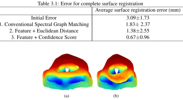
3.1 Error for complete surface registration . . . 39
3.2 Error for partial surface registration . . . 40
7.1 Surface registration error (mm) . . . 115
LIST OF FIGURES
1.1 CT/endoscopy fusion pipeline. . . 2
2.1 Charts on a 2D manifold. Two surface patches Uα, Uβ are respectively
parameterized viaφα, φβ. . . 11 2.2 Local representation of a map between manifolds.fis a differentiable map
betweenM1 andM2. fˆis the corresponding map represented on local charts. . . 12
2.3 The derivative of a differentiable mapf is a linear transformation(df)p
that maps a tangent vectorv ∈TpM1 to(df)p(v)∈Tf(p)M2. . . 13
2.4 A thin shell structure. . . 23
2.5 (a) General situation: in a infinitesimal local region, a vectora is trans-formed intox. (b) Thin shell: the third coordinate direction (z-direction)
overlaps with the normal direction. . . 24
3.1 (a) Local geometry from which the geometric signaturef(v)is computed. (b) A vertexv, indicated as the cross point, is selected inM1. The feature
descriptor (the same one as shown in part (a)) is deployed onvto get the geometric feature vectorf(v). (c) The value of theithrow in the confidence score array ∆is plotted onM2 (red indicates large value). v0 ∈ M2 is
regarded as the most similar point tov ∈ M. . . 29 3.2 (a)M1 is uniformly colored. The overall correspondences are indicated by
the corresponding color inM2. (b) Correspondences derived from direct
feature matching via confidence scores. (c) Correspondences derived from
geometric-feature-based spectral graph matching. . . 33
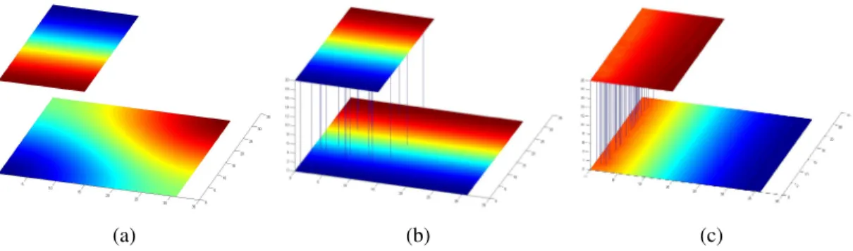
3.3 (a) Separate spectral decompositions are respectively applied to two sur-faces. The top surface is half of the bottom complete surface. The first eigenmode of each eigendecomposition is respectively color-coded on that surface. (b) A joint spectral decomposition is applied on an association graph connected by a sparse set of initial links. The color-coding shows the first joint eigenmode. (c) A joint spectral decomposition is applied on an association graph with initial links only on one side.Conclusion: only Fig.
b shows the desired eigenmode for the matching between the two surfaces. . . 36 3.4 The color-coded correspondences (a,b) between a complete surface and a
partial surface with a hole and truncation. (c,d) between surfaces with a
3.5 (a) A CT segmentation surface. (b) A synthetically deformed surface created from the surface in Figure a. The deformation includes the opening
of the epiglottis and the contraction of the pharyngeal wall. . . 39
3.6 The same surface pair as shown in Fig. 3.5 except that some holes and
truncation were added to (a). . . 40
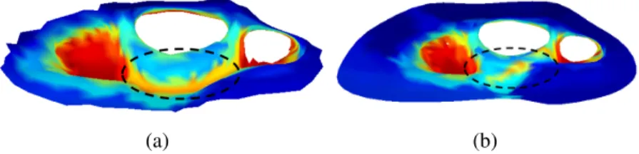
3.7 (a) A CT segmentation surface. (b) A bridge is manually created between the epiglottis tip and the pharyngeal wall. The circled regions indicate
inaccurate matching. . . 40
3.8 (a) A pharyngeal CT segmentation surface. (b) An endoscopic video reconstruction surface. (c,d) Color-coded correspondences between the CT surface (c) and the reconstruction (d). The circled regions indicate the
bridging situation. . . 41
4.1 The Cauchy-Green strain tensorquantifies how an infinitesimal circle is
deformed into an infinitesimal ellipse. . . 46
4.2 (a) A triangle before deformation. The two edges are represented asv1,v2
under an arbitrary 2D local coordinate system. (b) After deformation, the two edges are represented asv01,v02 under another arbitrary 2D local
coordinate system. . . 46 4.3 A basis stencil used for computing the discrete shape operator. θi (i =
1,2,3)measures the dihedral angle between adjacent triangles, li is the length of edgei,ti is a unit tangent vector orthogonal to edgei, andAis
the triangle area.. . . 48
4.4 Five structural links (red) are manually placed between the frontal and posterior wall of the epiglottis. The structural energy is based on the links’
length change to preserve the epiglottal thickness. . . 49
4.5 (a) Original tessellation before registration (b) Deformed tessellation after registration using edge-based stencils (Pauly et al., 2005; Bergou et al., 2006) (c) Deformed tessellation after registration using triangle-based
stencils (Section 4.1.1 and 4.1.2) . . . 53
4.6 Registration error for 12 complete surface pairs. The center-point of each vertical bar is the surface registration error, which is defined as the average ofvertex registration error; the length of the error bar denotes the standard
4.8 From left to right: deformable surface before registration; static surface; initial overlay between the two surfaces before registration.; final overlay
between the two surfaces after registration; deformable surface after registration. . . . 56
4.9 Experimental setup for the phantom case: a real-size static 3D-printed model was produced from a CT segmentation of a real patient. We took endoscopy and CT of the phantom model and produced its reconstruction and CT segmentation. TSD was used to find the deformation caused by
reconstruction artifacts. . . 57
4.10 TSD on the phantom case. From left to right: Endoscopic reconstruction;
CT surface before registration; Initial overlay; Final overlay; Registered CT. . . 57 4.11 TSD on the two real patient cases. From left to right: Endoscopic
recon-struction; CT surface before registration; Initial overlay; Final overlay;
Registered CT. . . 58 4.12 (a) Original epiglottis (b) Deformed epiglottis with structural links. (c)
Deformed epiglottis without structural links. . . 59
5.1 The construction of an endoscopogram involves three major steps: (a) Structure-from-Motion-and-Shading (SfMS); (b) geometry fusion; (c)
tex-ture fusion. . . 62 5.2 Structure-from-Motion-and-Shading diagram (figure from (Price et al., 2016)). . . 63
5.3 (a) 5 registered surfaces are overlaid together with the pink surface having a piece of outlier geometry (circled in black). (b) A direct geometry fusion
with the presence of outlier geometry creates an unreasonable result. . . 69
5.4 (a) Local point cloudN(v)around vertexv. (b) Robust quadratic fitting (red grid) to normalizedN(v). The outlier scores ofN(v)are indicated by
the color-coding. . . 70
5.5 (a) Color-coded outlier scoresW of all vertices inL. (b) The remaining point cloud after thresholding the ourlier scoresW. (c) The largest remain-ing component. (d) Fused surface created from the largest component of
the remaining point cloud after outlier geometry removal. . . 70
5.6 Each vertex of the fused surface R finds its corresponding vertex in a registered single-frame reconstructionR0
i and traces back the color in the corresponding texture imageFi. Some vertices (green, yellow, red) inR have ambiguity in choosing the corresponding frame because they have corresponding vertices in bothR0
1andR
0
2. . . 72
5.8 A phantom endoscopic video frame (left) and the fused geometry (right)
with color-coded deviation (in millemeters) from the ground truth CT surface. . . 75
5.9 OD plot on the point cloud of 20 surfaces (a) before registration; (b) after registration; (c) after outlier geometry removal. (d) The final
endosco-pogram. . . 76
5.10 Four endoscopograms produced by the entire pipeline. . . 76
6.1 Anatomy of the pharynx: the three tissue types shown above have different
anisotropic elasticity properties. . . 79
6.2 A thin shell model: for a local point, the elastic properties on the tangent plane (blue) are symmetric with respect to two natural axes. The local strains may be parameterized by any other orthogonal frame. The angle,θ,
between the two frames is known as the canonical angle. . . 82 6.3 A Gaussian MRF model with nodes (white) defined on the dual graph
(blue) of a triangle mesh. Nodej (triangleTj) is associated with unknown
variables(Cj, θj)and a set of observed variables{ϕαj, καj|α= 1...N} . . . 85 6.4 Illustration of discrete parallel transport between two neighboring triangles.
The black frames are the parametrization frames, and the colored frames are the natural axes. The natural axes ofTi (blue) are transported intoTj
and are compared with the natural axes ofTj (green). . . 87
6.5 (a) A reference bar-shaped surface. (b) The two ground truth Young’s mod-uli are respectively color-coded across the surface. Red regions indicate smaller Young’s moduli (more elastic). Each local Young’s modulus is associated with a natural axis direction (black vector fields) (c) A surface deformation can be derived by first fixing its two ends at designated posi-tions and by optimizing Eq. 7 using ground truth elasticity. (d) The group
of simulated deformationsΦ. . . 89
6.6 (a) Estimated Young’s moduli and the associated estimates of natural axes. (b) Simulated surface deformations derived from ground truth elasticity (blue wireframe), estimated elasticity (gray surface) and isotropic elasticity (red frame). (c) The two ground truth Young’s moduli (the orange curves)
and the two estimated Young’s moduli (the blue curves) on all faces. . . 89
6.7 A reference surface (gray surface) and one of its synthetic deformations
(red wireframe). . . 93 6.8 (a) Ground truth Young’s moduli along the two natural axes. The epiglottis
(blue region in the top figure) is set to be stiffer than the vallecula (yellow
6.9 Registration accuracy over registration iterations under different options. The 2nd-round orthotropic registration (blue curve) performs better than the1st-round isotropic registration (black). Meanwhile, it is only slightly worse than the results derived using ground truth elasticity parameters.
This means further iterations won’t improve the accuracy too much. . . 95
6.10 The2nd-round orthotropic registration performs better than the isotropic registration under different levels of noise. . . 95
6.11 (a) 3D endoscopogram surfaces reconstructed from video. Red circles indicate the arytenoid cartilage. Green circles indicate the epiglottis. (b)(c) Estimated Young’s moduli and the associated natural axes. . . 96
7.1 Different kinds of disparity between an endoscopogram and a CT surface. Red: missing patches in the endoscopogram due to occlusion. Blue: miss-ing parts in the CT surface due to the partial volume effect. Green: missmiss-ing parts in the CT surface due to tissue collapsing. . . 101
7.2 The initial alignment pipeline.. . . 103
7.3 Convergence curves of the average surface registration error. . . 116
7.4 Convergence curves of the average disparity estimation error. . . 117
7.5 The upper row and the bottom row respectively show two surfaces to be registered in one synthetic case. From left to right: ground truth indicator functions, mode-derived indicator functions, Monte-Carlo-derived indicator functions, uncertainty maps. . . 118
7.6 left: an endoscopogram. Middle: a stripe pattern is plotted on the endosco-pogram surface. Right: The stripe pattern is transferred to the CT surface using the resulting deformationsΦ1◦Φ−21. The cyan regions correspond to incompatible regions in the CT surface that do not have counterparts in the endoscopogram. . . 119
LIST OF ABBREVIATIONS
TSD Thin Shell Demons MRF Markov Random Field EM Expectation-Maximization FEM Finite Element Method HKS Heat Kernel Signatures
CT Computed Tomography
CGAL Computational and Geometry Algorithms Library SfS Shape-from-Shading
SfMS Shape-from-Motion-and-Shading SfM Structure-from-Motion
OD Overlapping Distance MAP Maximum-a-Posteriori
CHAPTER 1
Introduction
1.1 Pharyngeal Radiation Treatment Planning
Modern radiation therapy treatment planning relies on imaging modalities such as computed tomography (CT) to determine tumor location and spread. CT scans are preferred since it is an x-ray based technique that can capture normal-tissue/tumor characteristics (electron density) as seen by the treatment beams used in radiation oncology and be used directly for dose calculation (Pereira et al., 2014). CT images also provide anatomical information necessary for tumor localization and verification of the treatment plans. However, for head and neck cancer, CT may not fully reveal tumor locations due to limited spatial and intensity resolution. Specifically, in the case of pharyngeal cancer, evidence has been shown that the cancer begins in the flat, squamous cells that make up the lining surface of the anatomical structures in the nasopharynx (Wei and Kwong, 2010). This fact makes it more difficult for tumor detection and localization in CT because CT inherently does not image tissue boundaries (Zhang et al., 2014).
prohibiting direct 3D tumor localization. Moreover, reviewing the video is time-consuming, and the optical views do not provide the full geometric conformation of the throat.
Hence, a data fusion between CT and endoscopy would be helpful in producing improved tumor localization and likely better treatment plans; this has motivated doing the registration between the two imaging modalities. In the next section, I will briefly describe the overall pipeline for the fusion between a 3D CT image and an endoscopic video, and I will point out the need for surface registration that is used in this pipeline.
1.2 CT/Endoscopy Fusion Pipeline
Given a 3D head-and-neck CT scan of a patient and a nasopharyngoscopic video of the same patient, the goal of the fusion is to transfer the texture and location information extracted from the endoscopic video into the CT space.
The general idea is to register an endoscopy-reconstructed 3D surface model with a CT segmentation surface. Fig. 1.1 shows the overall pipeline. The pipeline can be generally divided into the two following steps.
i. A 3D surface model, which we call anendoscopogram, is built from the endoscopic video using many 2D video frames. To do this, a partial 3D surface model is reconstructed for each
individual 2D frame. Then multiple single-frame-based partial 3D reconstructions are registered together to achieve a complete pharyngeal surface model (endoscopogram).
ii. The endoscopogram is registered to the 3D pharyngeal surface segmented out from the CT scan. The computed deformation between the two surfaces allows the transfer of tumor location and texture information from the endoscopogram to the CT space.
The above two steps require accurate surface registration. Surface registration is a long-studied topic (Audette et al., 2000) in the medical image computing field, and many promising methods have been proposed for various applications (Tam et al., 2013). Unfortunately, none of them suits the CT/endoscope fusion pipeline. The next section elaborates on some special challenges we have to face in our surface registration problem.
1.3 Challenges of Surface Registration for the Fusion
Surface Disparity. As mentioned above, the endoscopogram is built from multiple single-frame-based reconstructions. The challenge here for the surface registration is that all individual single-frame-based reconstructions are only partially overlapping with each other due to the con-stantly changing camera viewpoint across frames. Moreover, the individual reconstructions may have missing data (holes) due to camera occlusion. Despite the missing data situation, there is also a significant disparity between the endoscopogram and the CT surface. Because of the partial volume effect on CT and tissue collapse caused by pharyngeal deformations, there are surface patches in either the CT surface or the endoscopogram that do not have counterparts. This fact requires us to have a surface registration method that can handle partial data, different surface topology and other disparity problems. However, many surface registration algorithms are purely based on matching intrinsic surface geometry, thereby not suitable in our application.
groupwise surface registration method that can simultaneously register all the frames to a single target. Current groupwise methods rely on having a known template or iteratively estimating the mean surface. However, neither approach is feasible in our application due to the only partially overlapping nature of the single-frame reconstructions.
Large Nonrigid Deformation.Another challenge in building the endoscopogram is that one needs to take into account the fact that all single-frame-based reconstructions may be slightly deformed since the tissue may have deformed between 2D frame acquisitions. Such non-rigid tissue deformations, often caused by the swallowing motion of the patient during endoscopy, are physical processes governed by pharyngeal muscles. Other physical deformations in the pharynx come from the patient’s posture change between the CT scan time and the endoscopy time. During a CT scan, the patient is lying down on a curved table, whereas during endoscopy the patient is sitting straight up. Different gravity effects may cause significant shape changes in the pharynx, yielding large deformations between the endoscopogram surface and the CT segmentation surface. Finally, the presence of the endoscope can irritate the throat, leading to drastic pharyngeal motion. This mixture of different sources of deformations poses serious challenges to most current surface registration methods.
Physical Reality. Following the above argument, we prefer producing physically plausible deformations in the registration process. Unfortunately, most surface registration algorithms do not consider the physical properties of the surface material. Moreover, the apparent pharyngeal surface deformation is affected by the underlying muscles and bones. An accurate physical model there-fore requires comprehensive anatomical knowledge of the entire head-and-neck region, including material stiffness parameters of different tissue types. However, patient-specific measurements of these parameters are not obtainable in our application, which makes realistic physical modeling extremely challenging.
training/prediction procedure relies on the pure geometric appearance of the training examples, and physical reality is rarely considered in this line of thinking.
Initial Surface Alignment. The endoscopogram surface and the CT surface live in two unrelated Euclidean spaces respectively: the camera space and the CT imaging system coordinate space. They therefore differ by a similarity transform. We need to first determine that transformation before solving for the aforementioned non-rigid deformation. However, an endoscopogram only portrays that portion of the pharyngeal surface that is present in the endoscopic video, so the initial alignment (transformation, rotation, scaling) between this partial surface and a complete CT segmentation surface is made difficult. Simple alignment methods, such as Iterative Closest Point (ICP), will not suffice because of the additional large non-rigid deformations.
1.4 A Brief Outline of the Proposed Methods
With all the aforementioned challenges in mind, in this dissertation I investigate the surface registration problem under the context of CT/Endoscope fusion from three major perspectives: geometry, physics and statistics. With the consideration of all three aspects, my proposed method, Thin Shell Demons, can efficiently solve the surface registration problem in our application.
1.4.1
Geometric Feature Descriptor
I show that the feature matching strategy for surface registration can effectively handle partially overlapping surfaces with missing data and topology change.
1.4.2
Thin Shell Physical Model
We seek to produce physically plausible deformations from one surface to the other. This may require complex 3D physical modeling of the pharyngeal mechanics. To simply the problem, I propose to approximate 3D mechanics using the thin shell model, which concentrates only on the physical properties of 2D surface geometry. Results have shown that the thin shell model can produce reasonable registration results in our application while having a low computational cost. Based on the thin shell physical model, I propose a pairwise surface registration method, called Thin Shell Demons (TSD), that can be used to register the endoscopogram to the CT surface. In general, TSD constructs some virtual attraction forces between the two surfaces using geometric feature matching and computes a physically plausible deformation under the attraction. The method is robust against partial data and surface topology change.
1.4.3
Surface Disparity Estimation
1.4.4
Groupwise TSD
By mimicking the idea of N-body interaction, I extend TSD into a groupwise framework, where the attraction forces are computed among N surfaces and can gradually deform all the surfaces towards an implicit mean shape. The advantages of groupwise TSD over other groupwise frameworks include its template-free nature and the ability to handle partially overlapping surfaces with missing data and different topology. Groupwise TSD is well suited for registering many single-frame-based reconstructions into a unified piece of geometry (endoscopogram).
1.4.5
Anisotropic Elasticity Learning
1.5 Thesis and Contributions
Thesis: Geometric information and physical modeling can improve surface registration results in the context of CT/endoscopy fusion. The anisotropic parameters in the physical model can be
inferred probabilistically from a set of observed material deformations.
The contributions of this dissertation are as follows:
1. A novel geometric feature descriptor has been designed for discrete triangle meshes. This high-dimensional descriptor can capture multiscale curvature information of local shapes and provide the opportunity for advanced feature matching for matching pharyngeal shapes.
2. A geometric-feature-based spectral graph matching method has been proposed to compute dense correspondences between two partial surfaces. The method makes use of the aforementioned feature descriptor to produce initial correspondences for an improved joint spectral graph matching.
3. A surface registration method, called Thin Shell Demons, has been proposed to efficiently deal with partial surfaces with different topology. The method uses both geometric feature matching and a thin shell deformation model to produce physically plausible surface deformations.
4. A joint estimation framework based on Monte-Carlo Expectation-Maximization has been proposed to simultaneously estimate deformations and incompatible regions between the two surfaces.
5. A groupwise surface registration framework based on TSD has been proposed to robustly register many partially overlapping surfaces with missing patches. The framework mimics the N-body interaction principle and is template-free to deal with the challenge of mean surface estimation.
7. Based on the above elasticity learning framework, a joint estimation framework has been proposed to simultaneously estimate surface deformations in a groupwise registration setting and the elasticity parameters.
Besides the above methodological contributions, I have also accomplished the following engineering contributions:
1. A similarity transform fitting method has been designed to robustly compute an initial alignment between the partial endoscopogram surface and the complete CT surface.
2. A texture fusion algorithm has been designed to consistently stitch texture patches from multiple frames into a unified endoscopogram texture.
3. An overall pipeline for building an endoscopogram has been designed to effectively integrate reconstruction, geometry registration and texture fusion.
With the above scientific and engineering contributions, tumor transfer from an endoscopic movie to the CT space is enabled. To conclude, this dissertation develops necessary image computing techniques for making potential improvements in radiation treatment planning of pharyngeal cancer.
1.6 Overview of Chapters
CHAPTER 2
Background
This chapter presents some background required in this dissertation. In particular, mathematical background of differential geometry is briefly reviewed in Section 2.1. Background for surface registration algorithms is discussed in Section 2.2. Finally, some basic physics for 2D/3D elastic materials is reviewed in Section 2.3.
2.1 Geometry of Surfaces
This dissertation has to deal with surfaces represented by noisy discrete triangle meshes. How-ever, I will first review properties of continuous smooth curved surfaces, which are mathematically defined as 2-dimensionaldifferentiable manifolds. This will facilitate analysis of practical real-life problems, and we can in turn draw many useful insights from some of the well-developed theories. In this section, I will briefly review some mathematical definitions and properties of differentiable manifolds. Without loss of generality, we assume the manifold is 2-dimensional (surfaces), but the theories can be applied to higher dimensional manifolds.
2.1.1
Differentiable Manifold
The key entities investigated in this dissertation are smooth curved surfaces, such as endoscopic reconstruction surfaces and CT segmentation surfaces. Such surfaces are more often mathematically understood asdifferentiable manifolds. ADifferentiable Manifoldis a specific type oftopological manifold. The local surface is constrained to smoothly resemble a 2D Euclidean space, a 2D plane. Formally, a differentiable manifold is a topological manifold equipped with an equivalence class of
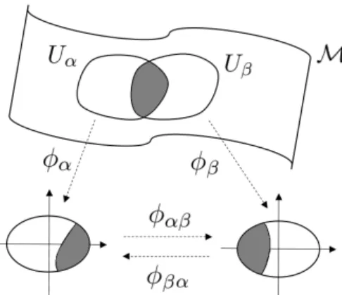
Figure 2.1: Charts on a 2D manifold. Two surface patchesUα, Uβ are respectively parameterized viaφα, φβ.
Anatlason a topological spaceMis a collection of pairs{(Uα, φα)}calledcharts, where the Uαare open sets that coverM, and for each indexα,
φα :Uα→R2 (2.1)
is a homeomorphism ofUαonto an open subset of2-dimensional real space. In other words, a chart serves as a 2D parameterization of the local surface ontoR2. Thetransition mapsof the atlas are
the functions
φαβ =φβ ◦φα|φα(Uα∩Uβ):φα(Uα∩Uβ)→φβ(Uα∩Uβ). (2.2)
If the atlas isC1 (allφα, φαβ areC1 differentiable), it is called a differentiable structure of a differentiable manifold. Intuitively, this definition (Fig. 2.1) reflects the notion of ”patching together pieces of flat spaces to make a manifold”. Different atlases (patchings) may produce “the same” manifold.
2.1.2
Differentiable Maps
Figure 2.2: Local representation of a map between manifolds. f is a differentiable map between M1andM2. fˆis the corresponding map represented on local charts.
point on the first surface to a point on the second surface. (The background of surface registration algorithms is given in Section 2.2.) Formally, letM1 andM2 be two 2D differentiable manifolds.
A mapf :M1 → M2 is said to be differentiable at a pointp∈ M1if there exist parameterizations
(U, φ)ofM1 atp(i.e.,p∈φ(U)) and(V, ψ)ofM2 atf(p), withf(φ(U))⊂ψ(V), such that the
map
ˆ
f :=ψ−1◦f ◦φ:U ⊂R2 →
R2 (2.3)
is smooth. As Fig. 2.2 shows, this definition decomposes a global mapping function into local mapping functions parameterized on local pieces (charts).
As coordinate changes are smooth, this definition is independent of the parameterizations chosen at f(p)and p. A differentiable mapf : M1 → M2 between two manifolds is called a
diffeomorphismif it is bijective and its inversef−1 :M1 → M2 is also differentiable.
2.1.3
Tangent Spaces
Figure 2.3: The derivative of a differentiable mapf is a linear transformation(df)p that maps a tangent vectorv ∈TpM1 to(df)p(v)∈Tf(p)M2.
of local stretching parameters and local bending parameters. It turns out that tangent spaces are the most commonly used local flat spaces for such local parameterizations.
Recall from elementary vector calculus that a vectorv∈R3is said to betangentto a surfaceM
at a pointp∈ M2if there exists a differentiable curvec: (−, )such thatc(0) =pandc˙(0) =v.
The setTpMof all these vectors is a 2-dimensional vector space, called the tangent space toMat p, which can be identified with the plane inR3that is tangent toMatp.
Now we can parameterize a local manifold patch onto the tangent plane. Choosing a parame-terizationφ:U ⊂TpM → Maroundp, the curvecon the manifold can be mapped back to the tangent plane asˆc(t). Its coordinates on the tangent plane are given by
ˆ
c(t) := (φ−1◦c)(t) = (x1(t), x2(t))). (2.4)
Taking its derivative at pointp, we can write
˙
c(0) = ˙x1(0)( δ
δx1)p + ˙x
2(0)( δ
δx2)p, (2.5)
We now can talk about a differential map between two manifolds in terms of the collection of local transformations defined on the tangent plane. Letf : M1 → M2 be a differentiable map
between smooth manifolds. Forp∈ M1, the derivative off atpis the map
(df)p :=TpM1 →Tf(p)M2. (2.6)
It can be proven that(df)pis alineartransformation. In other words, as shown in Fig. 2.3,(df)p transforms a tangent vectorv∈TpM1into another tangent vector(df)p(v)∈TpM1.
2.1.4
Riemannian Manifolds
As mentioned in the last subsection, the deformation of a surface can be classified into two categories: stretching and bending. Between those two, the stretching deformation will always alter the distance measurement between two points on the surface; this is an important phenomenon in this study. In the standard 3D Euclidean space the metric properties of distances are determined by the canonical Cartesian coordinates. In a general differentiable manifold, however, there are no such preferred coordinates to define distances, angles and volumes. We must rely on a new structure, a special tensor field called theRiemannian metric.
A Riemannian metric on a manifoldMis a function that smoothly assigns to each point p∈ Ma symmetric positive definite 2-tensorg on the tangent spaceTpM. The tensorgis called a metric tensor; it defines how distances are measured locally. Ifx:V →R2is a local chart, we have
g =
n X
i,j=1
gijdxi⊗dxj, (2.7)
inV, wheredxiis the 1-norm associated with( δ δxi)and
gij =h( δ δxi),(
δ
A smooth manifoldMequipped with a Riemannian metric g is called aRiemannian manifold, and is denoted by(M, g).
A Riemannian metric allows us to compute the length||v|| =< v, v >12= pgp(v, v)of any vectorv∈ TpM. Therefore we can measure the length of a curvec: [a, b]→ Mby integrating along its path
l(c) =
Z b
a
||c˙(t)||dt. (2.9)
If two manifolds are equipped with identical Riemannian metrics, they are regarded asisometric. Formally, let (M1, g) and (M2, h)be two Riemannian manifolds equipped with metrics g and
h respectively. A diffeomorphism f : M1 → M2 is said to be an isometry if f ◦ h = g,
i.e., the metrics are identical after the mapping. This also means thatf doesn’t change distance measurement between the two manifolds, i.e.,d(p, q) = d(f(p), f(q)), whered(·,·)is the distance function between two points on the manifold.
The algebraic form of the metric tensorg is different under different parameterizations. For a point p ∈ M, a special parametrizationφp : U → R2 is called canonical if the metric tensor gp is the identity matrix. Now let us consider a diffeomorphic mapf :M1 → M2 between two
Riemannian manifolds. For a pair of correspondencesp→q,p∈ M1 andq =f(p)∈ M2, letgp andgqbe their respective metric tensors under canonical parameterization. We have the following transformation:
gp =JpTgqJp, (2.10)
whereJpis the Jacobian of(df)p (derivative off atp, which is a linear transformation defined on TpM1). In particular, the matrixJpTJpcharacterizes how an infinitesimal circle is deformed into an infinitesimal ellipse on the tangent plane. In physics, this matrix is understood as a tensor
=JpTJp−I, (2.11)
2.1.5
Levi-Civita Connection
In Chapter 5, in order to study the anisotropic directional information for elastic materials, the notion of smoothness of a vector field has to be defined on a manifold. In the Euclidean space, one way to measure the “smoothness” of vector fields is through the notion of directional derivatives. To be more specific, ifX andY are two vector fields in Euclidean space, we can define the directional derivative∇XY ofY alongX. Parallel transport of a vectorvalongXis expressed as∇Xv= 0, which means the direction ofvkeeps unchanged during the transport. This definition, however, uses the existence of Cartesian coordinates, which no longer holds in a general manifold. To overcome this difficulty we must introduce more structures.
TheLevi-Civita Connectiongeneralizes the idea of taking directional derivatives to manifolds. Intuitively, the parallel transport of a vector from one tangent plane to another on a manifold is done by first “unfolding” the local manifold to a flat space, then transporting the vector in a Euclidean fashion and finally ”folding” the flat space back to a manifold. Formally, the derivative vector
(∇XY)p ∈TpM, known as the covariant derivative ofY alongX, is computed as
∇XY = n X
i=1
(X·Yi+
n X
j,k=1
ΓijkXjYk) δ
δxi, (2.12)
where the form Xi indicates theith coordinate of the vector field X, andΓi
jk are theChristoffel
symbolsfor the Levi-Civita connection:
Γijk = 1 2
n X
l=1
gil(δgkl
δxj +δgjl δxk −δgjk δxl ) (2.13)
wheregij = (g−1
ij ).
differen-tiable curvecsuch thatV(t)∈Tc(t)M.Its covariant derivative alongcis given by
DV
dt (t) := ∇c˙(t)V = (∇XY)c(t). (2.14)
Then a vector fieldV defined along a curvecis said to beparallelalongcif DVdt (t) = 0.
With the definition of directional derivative, we can also generalize the notion of a ”straight line” to manifolds. To that end, a curvecis called ageodesicifc˙is parallel alongc, i.e., if Ddtc˙(t) = 0. Intuitively, geodesics serve as straight lines in Riemannian geometry. They are locally distance-minimizing paths; Thegeodesic distanced(p, q)between two pointspandqofMis defined as the infimum of the length taken over all continuous, piecewise continuously differentiable curves.
2.1.6
Curvature
Finally, the notion of surface ”curvedness” is constantly used throughout this dissertation. In the registration task, in order to build correspondences between two surfaces, similarly curved surface patches have to be first detected. Curvatures are well-defined for spatial curves. However, as discussed in Section 2.1.3, for a pointp∈ M, any tangent vectorv∈TpMcan be associated with a spatial curvec: (−, )such thatc˙(0) =v, which means that the curvatures are different atp along different tangent vector directions.
It turns out that the curvature at a pointpcan be fully encoded by thesecond fundamental form
II(u,v), algebraically represented by a2×2symmetric matrix:
[IIij] =
ω2hf1i ω1hf1i
ω2hf
2i ω1hf2i
(2.15)
where {f1,f2} stands for two orthogonal coordinate directions spanning the tangent plane, and
ωihf
With this definition, II(v,v)gives the curvature along directionvasvT[IIij]v. Theprincipal curvaturesatp, denotedk1 andk2, are the maximum and minimum values of this curvature, and
they are computed as the eigenvalues of[IIij]. The corresponding eigenvectors are theprincipal directions, vectors along which the principal curvatures are achieved. Note that both the algebraic form of [IIij] and the coordinates of principal directions are dependent on the choice of local parameterization (orthogonal basis).
TheGaussian curvatureatpis defined as the product of the two principal curvatures:K =k1k2,
and the mean curvature is defined as the mean of the two principal curvatures: H = (k1 +
k2)/2. Gaussian curvature and mean curvature are both very important curvature measurements, as
Gaussian curvature indicates the local surface type (hyperbolic, flat, elliptic) and mean curvature indicates local curvedness in average.
2.2 Surface Registration
The goal of surface registration (shape matching or alignment) is to find point-to-point cor-respondences between two or multiple geometric surfaces. This problem is a key algorithmic component in various tasks, such as 3D scan alignment and statistical medical shape analysis. Surface registration methods can be generally classified into two categories: rigid and non-rigid registration. Recently most research attention has been drawn to the non-rigid case because in many applications a rigid transformation can not sufficiently registration deformable objects. In fact, non-rigid registration problems are more ill-posed and thus require more complicated models. Therefore, this section only gives the background of existing non-rigid surface registration methods.
2.2.1
Matching-Based Methods.
pro-These methods usually can credibly find a set of correspondences at places that yield distinct and matchable feature descriptors. However, feature matching by itself may produce outliers, which can lead to an illegal or non-smooth global mapping between surfaces. Therefore, even though feature descriptors play an important role in the registration process, further mechanisms have to be incorporated to guarantee the correctness and smoothness of the global mapping. Higher-order graph constraints (Zeng et al., 2010) or higher-order Markov Random Fields (MRF) (Zeng et al., 2013) have been proposed, but these algorithms are NP-hard in nature and thus only feasible in small scale problems. In Chapter 3 I will introduce a new geometric feature descriptor that can help the registration and will show that it can be combined with other methods to produce smooth mappings.
2.2.2
Embedding-Based Methods.
MDS along with the idea of eigendecomposition on affinity matrices is indeed a powerful tool for surface matching. However, MDS requires a dense affinity matrix for preserving geodesic distances among all pairs of vertices. From Section 2.1.4, we can see that isometry can also be defined via identical Riemannian metrics. Based on this notion, the spectral matching method has shown its success by using the Laplace-Beltrami operator instead of the dense affinity matrix to perform eigendecomposition (Zigelman et al., 2006; Balci et al., 2007; Reuter, 2010). Closely related to the Riemannian metric, the Laplace-Beltrami operator is defined only from local surface geometry, so its discrete version has a sparse matrix structure, allowing fast computation for surfaces with hundreds of thousands of vertices. Other variants along this line of thinking are based on graph Laplacian (Lombaert et al., 2011; Mateus et al., 2008) and Laplace-Beltrami functional spaces (Pokrass et al., 2013; Ovsjanikov et al., 2012). Generally speaking, all these methods rely on surfaces having the same intrinsic geometry (isometry) and can only handle bending deformations between surfaces. Moreover, they certainly can not handle more complicated issues such as surface topology change or the existence of missing surface patches (partial data).
Conformal mapping (Gu et al., 2004) and the M¨obius transformation (Lipman and Funkhouser, 2009) can be used to deal with near-isometry situations by relaxing the geodesic-preserving con-straint to the angle-preserving concon-straint. Quasi-conformal mapping (Lam et al., 2014; Zeng and Gu, 2011) has also been proposed to handle the most general diffeomorphic situation. However, these methods mostly require the surface to be genus-zero in order to be embedded into a common disc/sphere domain, and they have also not been shown to be effective in dealing with partial data and complicated topology change.
2.2.3
Deformation-Based Methods.
As discussed in the previous section, embedding-based methods are inherently not suitable for dealing with different intrinsic geometry. A better way to understand our registration problem is to seek a deformation that carries one surface closer to the other. This will bypass the many geometric constraints needed in the embedding-based methods. Following this notion, the registration is formulated as an optimization over the set of possible deformations to minimize a function of two energy terms: data mismatch and deformation regularity. The first term, also known as data fidelity, encourages the optimized deformation field to carry one surface as close to the other as possible. The second term, also known as regularization, prefers to produce “realistic” surface deformations. Many approaches have been proposed to explore different formulations of these two terms.
Some works in registering 3D range scans (Pauly et al., 2005; Li et al., 2008) have been using the so-called closest-point rule, which refers to the strategy that each point on a surface is driven to the closest point on the other surface. Clearly, this strategy suffers with large deformations and inaccurate point positions. LDDMM (Bauer and Bruveris, 2011) and Currents (Vaillant and Glaun`es, 2005) have provided another elegant mathematical framework that produces diffeomorphic deformations between surfaces by comparing their normal fields. However, this framework still can not handle missing surface parts.
to be superior to the closest-point rule. Recently, Iglesias et. al. (Iglesias et al., 2013) developed a similar framework with implicit surface representation and a physically meaningful smoothness term by regarding the surface as a layer of an elastic material. However, the implicit presentation in these works requires embedding a surface into the ambient space using a signed-distance level-set function. However, voxelizing the 3D space can highly increase the data dimension and lacks the triangulation flexibility of surface meshes. Moreover, the signed-distance function itself is hard to track under large deformations.
Nevertheless, the Demons idea is still appealing because it has few assumptions about deforma-tion/surface properties; it does not require surface completeness and identical topology. Based on this observation, I will introduce in Chapter 4 a physics-based surface registration method called Thin Shell Demons.
2.3 Thin Shell Mechanics
The deformation of the pharyngeal tissues are physical processes caused by surrounding muscles and the forces on these tissues from the endoscope. A realistic physical model is then needed in a registration framework to produce such deformations. In our case, an endoscopic movie only sees the pharyngeal surface and the only CT information relevant to registration is that surface. Therefore, I propose to only model surface deformations. In particular, I adopt the thin shell physical model, which has been shown to be effective in the graphics literature (Gingold et al., 2004) to animate deformations of curved surface structures.
Figure 2.4: A thin shell structure.
For the purpose of analysis, a shell may be considered as a three-dimensional body, and the theory of linear elasticity may then be applied. However, this will generally be complicated and computationally demanding. In the theory of shells, an alternative simplified method is therefore employed. Based on some hypotheses made in the later sections, the 3D mechanics of a shell may be reduced to the analysis of its middle surface only. This also serves our purpose, which is to concentrate on the surface deformation instead of the whole 3D body.
For notational convenience in the following, we constrain subscripts denoted by Greek letters to have values in{1,2}, and those denoted by Roman letters to have values in{1,2,3}.
2.3.1
Strain-Displacement Relation for Thin Shells
General 3D Strain.Strain refers the relative displacement of particles in an infinitesimal area of an object. Suppose an elastic deformation transforms a vectora= [a1, a2, a3]intox= [x1, x2, x3].
In engineering, the strainEis a measurement of relative displacementds2−ds2
0, whereds0 is the
increment of initial length anddsis the increment of current length. Fig. 2.5 suggests the following relation
xi =ai+ui, dxi =dai+dui, ds=||da||, ds0 =||dx||, (2.16)
whereu= [u1, u2, u3]is the displacement vector. Then it is easy to get
(a) (b)
Figure 2.5: (a) General situation: in a infinitesimal local region, a vectorais transformed into x. (b) Thin shell: the third coordinate direction (z-direction) overlaps with the normal direction.
where Einstein summation is used in the above equation overi,j andk. In Eq. 2.17 the notation •,i represents the partial derivative with respect to the ith coordinate. From this equation the
Green-Lagrangian strain tensor is defined to be of the following form
E= [εij] =
ε11 ε12 ε13
ε21 ε22 ε23
ε31 ε32 ε33
(2.18)
where εij = uj,i +ui,j +ui,kuj,k. The notion of strain allows the measurement of local elastic deformation. In fact, we can see that given an arbitrary vectorv,vTEvgives the squared length change along thevdirection.
Thin Shell Strain Approximation. We place the coordinate system on a thin shell in such a way that the third coordinate direction (z-direction) overlaps with the normal and the first two coordinate directions span the tangent plane. We further assume the Love-Kirchhoff hypothesis is satisfied: the in-plane displacement is a linear function of the z-coordinate (out-of-plane coordinate): uα =u0α−zu3,α, whereu0αis the in-plane displacement (stretching) of the middle surface. With this hypothesis, Eq. 2.18 can be recast in the form (Ventsel and Krauthammer, 2001):
whereαβ = 12(u0α,β +u0β,α)is the 2D strain tensor of the middle surface, which is also known as the Cauchy-Green tangential strain tensor (Eq. 2.11). καβ =II0αβ −IIαβ is the shape operator (curvature) difference induced by the bending of the middle surface.
It has also been shown in (Ventsel and Krauthammer, 2001) that the strain tensor’s out-of-plane termsE3α, Eβ3, E33 can be negligible in the thin shell situation. In this way, the 3D strain of a
thin shell can be reasonably approximated using the 2D stretching and bending strain of its middle surface.
2.3.2
Thin Shell Deformation Energy
Coupled with strain is a physical quantity called stress, which expresses the internal forces that neighboring particles of an elastic material exert on each other. The existence of stress will induce potential energy, which I call thin shell deformation energy in our case. The measurement of such deformation energy plays an important role in my work. As will be discussed later, we prefer in many situations a low energy configuration of material deformations.
Hooke’s Law.In the modern theory of elasticity, the relation between strain and stress of an elastic material is summarized by Hooke’s Law:
[σ11, σ22, σ12]T =C[ε11, ε22, ε12]T, (2.20)
whereσαβ andεαβ are the in-plane stress and strain, andC is a3×3positive definite matrix, called astiffness matrix, characterizinglocalelasticity.
In the most common isotropic case, the elastic property of a local point is the same along all directions, and the stiffness matrix has the following simplified form:
C = E
1−ν2
1 ν 0
ν 1 0
0 0 (1−ν)/2
whereE is Young’s modulus, which represents the material’s stiffness, andνis the Poisson’s ratio, which represents the material’s compressibility.
For the isotropic case, it can be further shown that the local deformation energy of a point on a thin shell can be classified into two catergories: membrane (stretching) and bending. With Eq. 2.19, the membrane energy can be computed as
Wmembrane =
Eh
2(1−ν2)((1−ν)Tr(
2) +ν(Tr)2),
(2.22)
where Tr(·) stands for the trace operation andhis the shell thickness. The bending energy has a
similar form:
Wbending=
Eh3
24(1−ν2)((1−ν)Tr(κ 2
) +ν(Trκ)2). (2.23)
Then the total local energyW =Wmembrane+Wbending. Note that the above energy computation is only related to a single local point on the shell. To get the total deformation energy of an entire shell, one has to integrateW over the area of the shell:
Wtotal = Z
S
W dS (2.24)
Orthotropy.In the theory of elasticity mechanics, the termanisotropy, as opposed to isotropy, implies different elastic properties in different directions. In that case, the stiffness matrixCcan be an arbitrary3×3positive definite matrix with 6 free parameters. As a matter of fact, human tissue is mostly anisotropic (Kroon and Holzapfel, 2008). Therefore, the study of anisotropic elasticity becomes essential in realistic physical modeling.
system: C=
c1 c2 0
c2 c3 0
0 0 c4
= 1
1−ν12ν21
E1 ν21E1 0
ν12Ey E2 0
0 0 2G12(1−ν12ν21)
, (2.25)
where theEαare the Young’s moduli along the natural axes, theναβ are the Poisson’s ratios, and G12is the shear modulus.
Similar to the isotropic case, the local energy is the sum of the membrane and bending energy:
W = Eh
2(1−ν2)
TC+ Eh
3
24(1−ν2)κ
TCκ, (2.26)
CHAPTER 3
Geometric-Feature-Based
Spectral Graph Matching
The goal of surface registration is to seek a 3D deformation field that can aligncorresponding regionsin the two surfaces. Since a surface represents the boundary of an object of interest, these
corresponding regions are usually identified through distinguishable geometric shapes of local regions of the object. For example, in both the endoscopogram and CT surface, the epiglottis region appears as a convex curvy ridge, where the curvature along the sagittal direction is larger than that along the coronal direction. The pharyngeal wall in both surfaces is approximately cylindrical, where the curvature along the axial direction is very small. Therefore, the capability of describing local shapes is a fundamental building block of a successful surface registration method that seeks to match similar geometric structures.
(a) A local surface patch (b) M1 (c) M2
Figure 3.1: (a) Local geometry from which the geometric signaturef(v)is computed. (b) A vertex v, indicated as the cross point, is selected inM1. The feature descriptor (the same one as shown in
part (a)) is deployed onvto get the geometric feature vectorf(v). (c) The value of theithrow in the confidence score array∆is plotted onM2(red indicates large value). v0 ∈ M2is regarded as
the most similar point tov ∈ M.
3.1 Geometric Feature Descriptor
As discussed in Section 2.1, a surface is mathematically defined as a differentiable manifoldM. Without loss of generality, we assume the two principal directions and the associated two principal curvatures can be defined almost anywhere inM, with finite singular points, known as umbilics, where the curvature is the same along all directions (Koenderink, 1990).
We design a novel feature descriptorf to create ageometric signaturef(v)for a given point v ∈ M. Since local shape can be described by curvatures measured at different scales in a local region, the feature descriptorf is designed to collect curvature information on both its own location and a number of surrounding locations. As shown in Fig. 3.1a, for a given pointv, we find 8 surrounding points {vi |i = 1...8} by going along 8 equally angularly spaced geodesic directions {gi|i = 1...8} fromv by a certain distance d. The choice of the value of d will be discussed in Section 3.4. The two orthogonal geodesic directionsg1andg3 are respectively the two principal directionsp1 andp2. In order to capture curvatures at different scales, the descriptor is defined based on the curvature and normal information collected at the 9 points in the local patch: f(v) = (C,S,∆N,∆N1,5,∆N3,7). The signaturef(v)is detailed as follows.
two curvature measuresc, s, which are more informative in differentiating different type of shapes and are derivable from the two principal curvaturesk1, k2 in the following way:
c =
r k2
1+k22
2 (3.1)
s = −2
πarctan[(k1+k2)/(k1−k2)] (3.2)
Intuitively,cindicates the level of curvedness, andsindexes shape types, i.e., being convex, concave, hyperbolic or parabolic. These two curvatures are computed atv and the 8 surrounding points{vi |i= 1...8}to describe local curvatures, i.e.,C=c∪ {ci|i= 1...8},S=s∪ {si |i=
1...8}. Larger scale measures of curvature between each of the surrounding points and the center are computed as the magnitudes of the normal direction difference between each of the end points and the center point, i.e.,∆N={||n−ni||2 |i= 1...8}. Finally, normal direction differences between
two extreme endpoint pairs (v1,v5) and (v3,v7) are computed to describe the general shape structure,
i.e.,∆N1,5 =||n1−n5||,∆N3,7 =||n3−n7||.
Discretization. In the discrete setting, a surface is represented as a triangle meshM. With some abuse of notation, the feature descriptor is applied to each vertexvin the mesh. In this work, geometric properties like normal directions, principal directions and curvatures are estimated for all the vertices using theComputational and Geometry Algorithms Library(CGAL). The 8 geodesic directions are sampled on the tangent plane, and geodesic marching is performed by the discrete Levi-Civita parallel transport (Crane et al., 2010). Since in the discrete case the end point of a geodesic path can end up being an arbitrary point on a triangle, whereas curvatures can only be estimated at triangle vertices, I choose the nearest vertex to the end point of the geodesic path to be {vi |i= 1...8}. Fig. 3.1b shows a case where the descriptor is deployed on a vertex of a triangle
3.2 Feature Matching
With the novel multiscale curvature feature descriptorf, we can perform traditional feature matching techniques to find corresponding regions between two surfaces. Here I propose afeature distancemeasurement for comparing the similarity between two feature vectors. A naive way is to adopt theL2metric on the feature vector space, and the distance between the two feature vectors of
v anduis simply defined as||f(v)−f(u)||2.
This definition naturally assumes that the order of the 8 surrounding points is consistent between vandu. However, the two principal directions are only uniquely defined up to a 180-degree rotation,
which means that both{p1,p2}and{−p1,−p2}are valid principal direction pairs. In practice, this poses a problem that the principal directions might experience a sign change from place to place. Taking consideration of this, the distance is then defined as
min{||f(v)−f(u)||,||f(v)−f∗(u)||}, (3.3)
where f∗ represents the feature vector computed after rotating the principal directions by 180 degrees.
In our application, when the two surfaces are rigidly aligned, corresponding anatomical regions shouldn’t be spatially too far apart. Therefore, a soft Euclidean thresholdτ is added into the feature distance measurement, yielding
δ(v, u) = min{||f(v)−f(u)||,||f(v)−f∗(u)||}+α(1 +e−(||xv−xu||−τ))−1, (3.4)
where the second part is a sigmoid function penalizing a too large Euclidean distance||xv−xu|| between two corresponding vertices and whereαis a weighting factor. With this feature distance measurement, we can construct anN1×N2 distance 2D-arrayDbetween two surfacesM1,M2
Normalizing the Distance Array. Here an additional step is to normalize the distance array to be aconfidence array. When used for computing credible initial correspondences, the distance measurement is not commensurable across different regions. For example, the matching between two flat regions is highly ambiguous, but the feature distance is likely to be zero due to the small local curvatures. Distinguishable curved shapes are less ambiguous to match, but these places tend to yield larger feature distances. To summarize, in the original distance arrayD, small feature distances don’t correlate well with good matchings. To deal with this problem, I propose the following normalization technique.
The idea is to consider a confidence score that measures how likely{vi ∈ M1, uj ∈ M2}is a
pair in correspondence. We consider both-way corresponding likelihoods measured byδ1
i,j andδ2i,j respectively. δ1
i,j is defined as the likelihood ofuj ∈ M2 being the most similar vertex ofvi ∈ M1,
compared to all other vertices inM2. A simple way to compute this quantity is to normalize theith
row ofDto the range of[0,1].
δi,j1 = 1−(δ(i, j)−min
k δ(i, k))/(maxk δ(i, k)−mink δ(i, k)). (3.5)
δ2
i,j is defined and computed vice versa:
δi,j2 = 1−(δ(i, j)−min
k δ(k, j))/(maxk δ(k, j)−mink δ(k, j)) (3.6)
Because the two likelihoods are now at the same scale, the confidence score∆i,jis computed by taking the sum ofδi,j1 andδ2i,j. All the confidence scores will form aN1×N2confidence score
array∆. As shown in Fig. 3.1b and Fig. 3.1c, for the vertexvi selected inM1, theith row in∆is
color-coded inM2. The vertex with the largest value is selected as the corresponding point. The
(a) M1 (b) M2 (c)M2
Figure 3.2: (a)M1 is uniformly colored. The overall correspondences are indicated by the
corre-sponding color inM2. (b) Correspondences derived from direct feature matching via confidence
scores. (c) Correspondences derived from geometric-feature-based spectral graph matching.
∆and add(vi, vj)to the initial correspondence set. To avert non-one-to-one correspondences, we zero out theith row andjth column of∆after each selection. I repeat this procedurettimes to select thetmost credible correspondences.
3.3 Geometric-Feature-Based Spectral Graph Matching
3.3.1
Spectral Graph Matching on an Association Graph
Two graphsG1 ={V1,E1}andG2 ={V2,E2}can be constructed from the two surfacesM1
andM2with the vertices and edges of their triangle meshes. Anassociation graphG={V,E}is
built by connectingG1andG2with a set of initial links. Gis equipped with an|N1+N2| × |N1+N2|
affinity array W, where the affinitieswi,j between vertexi and vertexj are measured using the Euclidean distance between two vertices in the original 3D space for both intra-surface links and inter-surface links; that is,wi,j =||xi−xj||−2if∃ei,j ∈E. WithVbeing the ordered pair(V1,V2),
Wtakes the form of
W1 W21
W12 W2
(3.7)
whereW1,W2are intra-surface affinities andW12andW21are inter-surface affinities. Thegraph
LaplacianoperatorLis defined asL=D−W, whereDis a diagonal array withdi = P
jwi,j. The spectral decomposition ofLprovides an orthogonal set of eigenvectors[u1,u2, ...,u|N1+N2|] with corresponding non-decreasing eigenvalues. The first eigenvector is always constant with an associated zero eigenvalue; it is not useful for our matching purpose. Then thespectral embedding
of the graph into ak-dimensional Euclidean space (spectral domain) is given by[u2,u3, ...,uk+1]. Formally, we defineF= [f1,f2, ...,fk]as an|N1+N2| ×karray. Then the firstkeigenmodes with
non-zero eigenvalues[u2,u3, ...,uk+1]is the solution to the following minimization problem:
arg min
f1,f2,...,fk
|N1+N2| X
i,j=1
wi,j kf(i)−f(j) k2, withFTF=I (3.8)
wheref(i)is theithrow ofF, representing the embedded Euclidean coordiantes (spectral represen-tation) of theithvertex. Intuitively, thekeigenmodes define an embedding into ak-dimensional Euclidean space that tries to respect the edge lengths of the graph. In other words, the distance between neighboring vertices in the embedded domain, computed by||f(i)−f(j)||, is close to that
Moreover, each eigenvectorui, known as theithvibration mode of graphG, can be separated into two functions: ui
1, the firstN1 values ofui, representing theith vibration mode ofG1, andui2,
the last N2 values of ui, representing the ith vibration mode ofG2. In fact, the aforementioned
spectral embedding of the association graphGsimultaneously embeds both graphsG1,G2into the
same spectral domain. As mentioned in (Lombaert et al., 2013), this association-graph-based spectral embedding provides several advantages over separate spectral embeddings. In particular, it solves the eigenvector permutation problem, namely that the order of eigenvectors often changes when they are associated with similar eigenvalues. Here, the inter-surface links of the association graph ensure that the combined eigenvectoruiincludes consistent vibration modes(ui
1,ui2)from
both graphs.
After knowing the spectral coordinates for all vertices, the final matching between the two surfaces is accomplished by a nearest-neighbor search in the k-dimensional spectral domain. Note that this method only yields a dense matching as a result but does not explicitly produce deformation fields between surfaces.
3.3.2
Geometric-Feature-Based Affinity Matrix
The inter-surface affinity in the Lombaert paper was defined according to the Euclidean distance between vertices, which is conceptually unnatural, because in most large deformation situations, two corresponding vertices might have a large Euclidean distance, ending up with a small affinity, even though there is a clear evidence showing the correspondence is correct and should have a high affinity. Therefore, I propose to compute the inter-surface affinity based on the confidence score of the initial correspondences derived by geometric feature matching. Withtinitial correspondences selected via the algorithm in Section 3.2, the affinity arrayW is now defined as
wi,j =
||xi−xj||−2 ifvi, vj are in same the surface,
The final matching result is shown in Fig. 3.2c. As we can see, the correspondences are smoother than from the feature matching directly.
3.3.3
Different Intrinsic Geometry
In our application, the two surfaces have different intrinsic geometry, such as different boundary locations and holes. Conventional separated spectral decompositions (Lombaert et al., 2011) in this situation will yield two totally different sets of eigenmodes. Just think of the simplest partial surface problem in Fig. 3.3a, in which one surface is a half of the other one. The first eigenmodes have distinct patterns, because surfaces with different sizes have different vibration modes. However, if only 5% of all the initial correspondences are assigned between the two surfaces, as shown in Fig. 3.3b, the first eigenmodes become consistent with each other. Intuitively, a joint vibration can be achieved by associating the partial surface onto the other one using the initial links, so that the partial surface is forced to vibrate together with the other. Moreover, it is already obvious in the objective function (Eq. 3.8) that the energy is minimized when both intra-surface and inter-surface affinities are preserved in the spectral domain, which means corresponding vertices have similar embedded coordinates, as well as vibration properties.
(a) (b) (c)