arXiv:1509.05206v1 [cond-mat.quant-gas] 17 Sep 2015
F. Tsitoura,1Z. A. Anastassi,2 J. L. Marzuola,3 P. G. Kevrekidis,4, 5and D. J. Frantzeskakis1 1
Department of Physics, University of Athens, Panepistimiopolis, Zografos, Athens 15784, Greece
2Department of Mathematics, Statistics and Physics, College of Arts and Sciences, Qatar University, 2713 Doha, Qatar 3
Department of Mathematics, University of North Carolina, Chapel Hill, NC 27599, USA 4
Department of Mathematics and Statistics, University of Massachusetts, Amherst, Massachusetts 01003-4515 USA 5Center for Nonlinear Studies and Theoretical Division,
Los Alamos National Laboratory, Los Alamos, NM 87544
We study dark solitons near potential and nonlinearity steps and combinations thereof, forming rectangular barriers. This setting is relevant to the contexts of atomic Bose-Einstein condensates (where such steps can be realized by using proper external fields) and nonlinear optics (for beam propagation near interfaces separating optical media of different refractive indices). We use perturbation theory to develop an equivalent particle theory, describing the matter-wave or optical soliton dynamics as the motion of a particle in an effective potential. This Newtonian dynamical problem provides information for the soliton statics and dynamics, including scenarios of reflection, transmission, or quasi-trapping at such steps. The case of multiple such steps and its connection to barrier potentials is also touched upon. Our analytical predictions are found to be in very good agreement with the corresponding numerical results.
PACS numbers: 03.75.Lm, 05.45.Yv
I. INTRODUCTION
The interaction of solitons with impurities is a fundamen-tal problem that has been considered in various branches of physics – predominantly in nonlinear wave theory [1] and solid state physics [2] – as well as in applied mathematics (see, e.g., recent work [3] and references therein). Especially, in the framework of the nonlinear Schr¨odinger (NLS) equa-tion, the interaction of bright and dark solitons with δ-like impurities has been investigated in many works (see, e.g., Refs. [4–8]). Relevant studies in the physics of atomic Bose-Einstein condensates (BECs) have also been performed (see, e.g., Refs. [9–13]), as well as in settings involving potential wells [14, 15] and barriers [16, 17] (see also Ref. [18] for ear-lier work in a similar model). In this context, localized impu-rities can be created as focused far-detuned laser beams, and have already been used in experiments involving dark solitons [19, 20]. Furthermore, experimental results on the scattering of matter-wave bright solitons on Gaussian barriers in either
7Li [21] or85Rb [22] BECs have been reported as well. More
recently, such soliton-defect interactions were also explored in the case of multi-component BECs and dark-bright soli-tons, both in theory [23] and in an experiment [24].
On the other hand, much attention has been paid to BECs with spatially modulated interatomic interactions, so-called “collisionally inhomogeneous condensates” [25, 26]; for a re-view with a particular bend towards periodic such interac-tions see also Ref. [27]). Relevant studies in this context have explored a variety of interesting phenomena: these in-clude, but are not limited to adiabatic compression of matter-waves [25, 28], Bloch oscillations of solitons [25], emission of atomic solitons [29, 30], scattering of matter waves through barriers [31], emergence of instabilities of solitary waves due to periodic variations in the scattering length [32], formation of stable condensates exhibiting both attractive and repulsive interatomic interactions [33], solitons in combined linear and nonlinear potentials [34–38], generation of solitons [39] and
vortex rings [40], control of Faraday waves [41], vortex dipole dynamics in spinor BECs [42], and others.
Here, we consider a combination of the above settings, namely we consider a one-dimensional (1D) setting involv-ing potential and nonlinearity steps, as well as pertinent rect-angular barriers, and study statics, dynamics and scattering of dark solitons. In the BEC context, recent experiments have demonstrated robust dark solitons in the quasi-1D set-ting [43]. In addition, potential steps in BECs can be realized by trapping potentials featuring piece-wise constant profiles (see, e.g., Refs. [44, 45] and discussion in the next Section). Furthermore, nonlinearity steps can be realized too, upon em-ploying magnetically [46] or optically [47] induced Feshbach resonances, that can be used to properly tune the interatomic interactions strength – see, e.g., more details in Refs. [30, 35] and discussion in the next Section.
version of such a setting has been touch upon in Ref. [35]. It is our purpose, in this work, to address this problem. In particular, our investigation and a description of our presen-tation is as follows. First, in Sec. II, we provide the descrip-tion and modeling of the problem; although this is done in the context of atomic BECs, our model can straightforwardly be used for similar considerations in the context of optics, as mentioned above. In the same Section, we apply perturbation theory for dark solitons to show that, in the adiabatic approx-imation, soliton dynamics is described by the motion of an equivalent particle in an effective potential. The latter has a tanh-profile, but – in the presence of the nonlinearity step – can also exhibit an elliptic and a hyperbolic fixed point. We show that stationary soliton states do exist at the fixed points of the effective potential, but are unstable (albeit in different ways, as is explained below) according to a Bogoliubov-de Gennes (BdG) analysis [57, 58] that we perform; we also use an analytical approximation to derive the unstable eigenvalues as functions of the magnitudes of the potential/nonlinearity steps. In Sec. III we study the soliton dynamics for various parameter values, pertaining to different forms of the effective potential, including the case of rectangular barriers formed by combination of adjacent potential and nonlinearity steps. Our numerical results – in both statics and dynamics – are found to be in very good agreement with the analytical predictions. We also investigate the possibility of soliton trapping in the vicinity of the hyperbolic fixed point of the effective poten-tial; note that such states could be characterized as “surface dark solitons”, as they are formed at linear/nonlinear inter-faces separating different optical or atomic media. We show that quasi-trapping of solitons is possible, in the case where nonlinearity steps are present; the pertinent (finite) trapping time is found to be of the order of several hundreds of millisec-onds, which suggests that such soliton quasi-trapping could be observable in real BEC experiments. Finally, in Sec. IV we summarize our findings, discuss our conclusions, and provide provide perspectives for future studies.
II. MODEL AND ANALYTICAL CONSIDERATIONS
A. Setup
As noted in the Introduction, our formulation originates from the context of atomic BECs in the mean-field picture [57]. We thus consider a quasi-1D setting whereby matter waves, described by the macroscopic wave functionΨ(x, t), are oriented along the x-direction and are confined in a strongly anisotropic (quasi-1D) trap. The latter, has the form of a rectangular box of lengthsLx≫ Ly =Lz ≡L⊥, with
the transverse length L⊥ being on the order of the healing
lengthξ. Such a box-like trapping potential, Vb(x), can be
approximated by a super-Gaussian function, of the form:
Vb(x) =V0
h
1−exp−x
w
γi
, (1)
whereV0andwdenote the trap amplitude and width,
respec-tively. The particular value of the exponentγ ≫ 1 is not
especially important; here we useγ = 50. In this setting, our aim is to consider dark solitons near potential and nonlinearity steps, located atx= L. To model such a situation, we start from the Gross-Pitaevskii (GP) equation [57, 58]:
i~∂Ψ
∂t =
h
− ~ 2
2m∂
2
x+g(x)|Ψ| 2
+V(x)iΨ, (2) Here,Ψ(x, t)is the mean-field wave function,mis the atomic mass,V(x)represents the external potential, whileg1D(x) = (9/4L2
⊥)g3D is the effectively 1D interaction strength, with
g3D= 4π~2α(x)/mbeing its 3D counterpart andα(x)being
the scattering length (assumed to beα >0,∀x, corresponding to repulsive interatomic interactions). The external potential and the scattering length are then taken to be of the form:
V(x) = Vb(x) +
(
VL, x < L
VR, x > L
, (3)
α(x) =
(
αL, x < L
αR, x > L
, (4)
whereVL,RandαL,Rare constant values of the potential and
scattering length, to the left and right ofx=L, where respec-tive steps take place.
Notice that such potential steps may be realized in present BEC experiments upon employing a detuned laser beam shined over a razor edge to make a sharp barrier, with the diffraction-limited fall-off of the laser intensity being smaller than the healing length of the condensate; in such a situa-tion, the potential can be effectively described by a step func-tion. On the other hand, the implementation of nonlinear-ity steps can be based on the interaction tunabilnonlinear-ity of spe-cific atomic species by applying external magnetic or optical fields [46, 47]. For instance, confining ultracold atoms in an elongated trapping potential near the surface of an atom chip [59] allows for appropriate local engineering of the scatter-ing length to form steps (of varyscatter-ing widths), where the atom-surface separation sets a scale for achievable minimum step widths. The trapping potential can be formed optically, pos-sibly also by a suitable combination of optical and magnetic fields (see Ref. [35] for a relevant discussion).
Measuring the longitudinal coordinate xin units of √2ξ (whereξ≡~/√2mng1Dis the healing length), timetin units
of√2ξ/cs(wherecs≡pg1Dn/mis the speed of sound and
nis the peak density), and energy in units ofg1Dn, we cast
Eq. (2) to the following dimensionless form (see Ref. [60]):
i∂u ∂t = −
1 2
∂2u
∂x2 +
α(x)
αL |
u|2
u+V(x)u, (5)
whereu=√nΨ. Unless stated otherwise, in the simulations below we fix the parameter values as follows: V0 = 10and
w= 250(for the box potential),VL= 0andVR=±0.01for
the potential step, as well asαL = 1andaR∈[0.9, 1.1]for
the nonlinearity step. Nevertheless, our theoretical approach is general (and will be kept as such in the exposition that fol-lows in this section).
the complex electric field envelope,tis the propagation dis-tance andxis the transverse direction, whileV(x)andα(x)
describe the (transverse) spatial profile of the linear and non-linear parts of the refractive index [36]. This way, Eq. (5) can be used for the study of optical beams, carrying dark solitons, near interfaces separating different optical media, with (dif-ferent) defocusing Kerr nonlinearities.
B. Perturbation theory and equivalent particle picture
Assuming that, to a first approximation, the box potential can be neglected, we consider the dynamics of a dark soliton, which is located in the regionx < L, and moves to the right, towards the potential and nonlinearity steps (similar consider-ations for a soliton located in the regionx > Land moving to the left are straightforward). In such a case, we seek for a solution of Eq. (5) in the form:
u(x, t) = pµL−VLexp (−iµLt)υ(x, t), (6)
where µL is the chemical potential, and the υ(x, t) is the
wavefunction of the dark soliton. Then, introducing the trans-formationst → (µL−VL)tandx →
√
µL−VLx, we
ex-press Eq. (5) as a perturbed NLS equation for the dark soliton:
i∂υ ∂t +
1 2
∂2υ
∂x2 − |υ| 2
−1
υ = P(υ). (7)
Here, the functional perturbationP(υ)has the form:
P(υ) = A+B|υ|2
υH(x−L), (8)
whereHis the Heaviside step function, and coefficientsA,B are given by:
A = VR−VL
µL−VL
, B= αR
αL −
1. (9)
These coefficients, which set the magnitudes of the potential and nonlinearity steps, are assumed to be small. Such a situ-ation corresponds, e.g., to the case whereµL = 1,VL = 0,
VR ∼ ǫ, and aR/αL ∼ 1, where 0 < ǫ ≪ 1 is a formal
small parameter (this choice will be used in our simulations below). In the present work, we assume that the jump from left to right is “sharp”, i.e., we do not explore the additional possibility of a finite width interface. If such a finite width was present but was the same between the linear and nonlin-ear interface, essentially the formulation below would still be applicable, with the Heaviside function above substituted by a suitable smoothened variant (e.g. atanhfunctional form). A more complicated setting deferred for future studies would involve the existence of two separate widths in the linear and nonlinear step and the length scale competition that that could involve.
Equation (7) can be studied analytically upon employing perturbation theory for dark solitons (see, e.g., Refs. [61– 63]): first we note that, in the absence of the perturbation(8), Eq. (7) has a dark soliton solution of the form:
υ(x, t) = cosφtanhX+isinφ, (10)
whereX = cosφ[x−x0(t)]is the soliton coordinate,φis
the soliton phase angle(|φ| < π/2)describing the darkness of the soliton,cosφis the soliton depth (φ = 0 andφ 6= 0
correspond to stationary black solitons and gray solitons, re-spectively), whilex0(t)anddx0/dt= sinφdenote the
soli-ton center and velocity, respectively. Then, considering an adiabatic evolution of the dark soliton, we assume that in the presence of the perturbation the dark soliton parameters be-come slowly-varying unknown functions of timet. Thus, the soliton phase angle becomesφ → φ(t)and, as a result, the soliton coordinate becomesX = cosφ(t) x−x0(t)
, with dx0(t)/dt= sinφ(t).
The evolution of the soliton phase angle can be found by means of the evolution of the renormalized soliton energy, Eds, given by [61, 62]:
Eds = 1 2
Z ∞
−∞
h
|υx|2+ |υ|2−1 2i
dx. (11)
Employing Eq. (10), it can readily be found thatdEds/dt = −4 cos2
φ sinφ dφ/dt. On the other hand, using Eq. (7) and its complex conjugate, yields the evolution of the renormal-ized soliton energy: dEds/dt = −R
+∞
−∞ Pυ¯t+ ¯P υt
dx, where bar denotes complex conjugate. Then, the above ex-pressions fordEds/dtyield the evolution ofφ, namely
dφ dt =
1
2 cos2φsinφRe
nZ +∞
−∞
P(υ)¯υtdx
o
. (12)
Inserting the perturbation (8) into Eq. (12), and performing the integration, we obtain the following result:
dφ dt = −
1 4 A+B
sech2 L−x0
+ 1 8Bsech
4
L−x0
, (13)
where we have considered the case of nearly stationary (black) solitons withcosφ≈1(andsinφ≈φ). Combining Eq. (13)
with the above mentioned equation for the soliton velocity, dx0(t)/dt = sinφ(t), we can readily derive the following
equation for motion for the soliton center:
d2x 0
dt2 =−
dW dx0
, (14)
where the effective potentialW(x0)is given by:
W(x0) = − 1
8 2A+B
tanh L−x0
− 241 Btanh3
L−x0. (15)
C. Forms of the effective potential
B
B(2A+B)
x0
W(x
0
)
x
0 x0 x0
x 0
W(x
0
)
x 0
A>0 A<0
I I
II
III IV
V VI
VI
II V
IV III
0
-A
-2A
0
-A-2A
0
0 0
0
0
0 0
0
0
0
0
0
FIG. 1: Sketch showing domains of existence of fixed points of the effective potentialW(x0)(depicted by gray areas) forA >0(blue
line) andA <0(red line). The insetsI−III(IV−VI) show the form ofW(x0), starting from – and ending to – a small finite value of
non-linearity stepB, which is gradually decreased (increased) forA >0 (A < 0), cf. black arrows. Small rectangular (yellow) points indi-cate parameter values corresponding to the forms ofW(x0)shown
in the insetsI−VI.
enable the presence of fixed points and associated more com-plex dynamics; in the presence of solely a linear step, the dark soliton encounters solely a step potential, similarly to what is the case for its bright sibling [18]; see also below.
In fact, in our setting it is straightforward to find that there exist two fixed points, located at:
x0± = 1 2ln
−A∓p
−B(2A+B)
A+B
!
, (16)
forB(2A+B) < 0and−2A < B < −A, forA > 0, or
−A < B <−2A, forA <0. In Fig. 1 we plotB(2A+B)
as a function ofB, forA > 0(blue line) andA < 0 (red line). The corresponding domains of existence of the fixed points, are also depicted by the gray areas. Insets show typical profiles of the effective potentialW(x0), for different values
ofB, which we discuss in more detail below. From the figure (as well as from Eq. (16) itself), the saddle-center nature of the bifurcation of the two fixed points, which are generated concurrently “out of the blue sky” is immediately evident.
First, we consider the case of the absence of the nonlinear-ity step,B= 0, as shown in the insetsIandIVof Fig. 1, for A >0andA <0, respectively. In this case,W(x0)assumes
a step profile, induced by the potential step. This form is pre-served in the presence of a finite nonlinearity step, B 6= 0, namely for−A < B < 0and0 < B < −A, in the cases A >0andA <0, respectively.
A more interesting situation occurs when the nonlinearity step further decreases (increases), and takes values−2A < B <−AforA >0, or−A < B <−2AforA <0. In this case, the effective potential features a local minimum (maxi-mum), i.e., an elliptic (hyperbolic) fixed point, in the region x < 0(x > 0) forA > 0emerge (as per the saddle-center
x
-5 0 5
|
υ s
(x)|
2
-0.2 0 0.2 0.4 0.6 0.8 1 1.2
10
3
W(x
0 )
x
0+
ω
r
-0.05 0 0.05
ω
i
-0.03 -0.02 -0.01 0 0.01 0.02 0.03
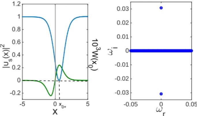
FIG. 2: (Color online) Left panel: density profile of the stationary soliton (blue line) at the hyperbolic fixed pointx0+= 0.66, as found
numerically, using the ansatzυs(x) = [1−V(x)]1/2tanh(x) in
Eq. (17), forαR/αL= 0.985,VR= 0.01,VL= 0,µL = 1; green
line illustrates the corresponding effective potentialW(x0). Right
panel: corresponding spectral plane (ωr,ωi) of the corresponding
eigenfrequencies, illustrating an exponential growth due to an imag-inary eigenfrequency pair.
bifurcation mentioned above) close to the location of the po-tential and nonlinearity steps, i.e., nearx = 0; a similar sit-uation occurs forA < 0, but the local minimum becoming a local maximum, and vice versa. The locationsx0±of the fixed
points are given by Eq. (16); as an example, using parameter valuesVL = 0,VR =−0.01,αL = 1andαR = 1.015, we
find thatx0+ = 0.66(x0− =−0.66) for the elliptic
(hyper-bolic) fixed point.
As the nonlinearity step becomes deeper, the asymptotes (forx→ ±∞) ofW(x0)become smaller and eventually
van-ish. For fixedVL = 0(andµL= 1), Eq. (15) shows that this
happens forB=−(3/2)A; in this case, the potential features a “spiky” profile, in the vicinity ofx = 0 (see, e.g., upper panel of Fig. 6 below). ForB < −(3/2)A, the asymptotes ofW(x0)become finite again, and take a positive (negative)
value forx < 0, and a negative (positive) value forx > 0, in the caseA > 0(A < 0). The spiky profile ofW(x0)in
the vicinity ofx = 0is preserved in this case too, but asB decreases it eventually disappears, as shown in the insetsIII
andVIof Fig. 1.
D. Solitons at the fixed points of the effective potential
The above analysis poses an interesting question regard-ing the existence of stationary solitons of Eq. (5) at the fixed points of the effective potential. To address this question, we use the ansatzu(x, t) = exp(−it)υs(x), for a stationary
soli-tonυs(x), and obtain from Eq. (5) the equation:
υs=−1 2
d2υ s
dx2 +
α(x)
αL |
υs|2υs+V(x)υs. (17)
x
-5 0 5
|
υ s
(x)|
2
-0.2 0 0.2 0.4 0.6 0.8 1 1.2
10
3
W(x
0 )
x
0-ω
r
-0.03 0 0.03
ω
i
×10-4
-2.5 -1.5 -0.5 0 0.5 1.5 2.5
FIG. 3: (Color online) Same as Fig. 2, but for a soliton located at the elliptic fixed pointx0−=−0.66; this state is found using the initial
ansatzυs(x) = [1−V(x)]1/2tanh(x+ 0.2). The spectral plane in
the right panel illustrates an oscillatory growth due to the presence of a complex quartet of eigenfrequencies.
numerically, by means of Newton’s method, employing the ansatz (forL= 0):
υs(x) = [1−V(x)]1/2tanh(x−x0). (18)
As shown in the left panel of Fig. 2, assuming an ansatz within Eq. (18) in which the soliton is initially placed atx0 = 0, we
find a steady state exactly at the hyperbolic fixed pointx0+= 0.66, as found from Eq. (16). On the other hand, the left panel of Fig. 3 shows a case where the initial guess is assumed in Eq. (18) to have a soliton positioned atx0 = −0.2, which
leads to a stationary soliton located exactly at the elliptic fixed pointx0−=−0.66predicted by Eq. (16).
It is now relevant to study the stability of these station-ary soliton states, performing a Bogoliubov-de Gennes (BdG) analysis [57, 58, 62]. We thus consider small perturbations of υs(x), and seek solutions of Eq. (17) of the form:
u(x, t) =e−it
υs(x) +δ b(x)e−iωt+ ¯c(x)eiωt¯ , (19)
where(b(x), c(x))are eigenmodes,ω =ωr+iωi are
(gen-erally complex) eigenfrequencies, and δ ≪ 1. Notice that the occurrence of a complex eigenfrequency always leads to a dynamic instability; thus, a linearly stable configuration is tantamount toωi= 0(i.e., all eigenfrequencies are real).
Substituting Eq. (19) into Eq. (5), and linearizing with re-spect toδ, we derive the following BdG equations:
ˆ
H−1 + 2α(x)
αL
υ2 s
b+α(x)
αL
υ2
sc=ωb, (20)
ˆ
H−1 + 2α(x)
αL
υ2 s
c+α(x)
αL
υ2
sb=−ωc, (21)
whereHˆ =−(1/2)∂2
x+V(x)is the single particle operator.
This eigenvalue problem is then solved numerically. Exam-ples of the stationary dark solitons at the fixed pointsx0±of
the effective potentialW, as well as their corresponding BdG spectra, are shown in Figs. 2 and 3. It is observed that the solitons are dynamically unstable, as seen by the presence of
1-B
1.01 1.012 1.014 1.016 1.018 1.02
ω
i0 0.01 0.02 0.03
1-B
1.01 1.012 1.014 1.016 1.018 1.02
ω
i
×10-4
0 1 2 3
1-B
1 1.15 1.3 1.45 1.6
ω
r0 0.05 0.1 0.15 0.2 0.25
FIG. 4: (Color online) Top panel: the imaginary part of the eigen-frequency,ωi, as a function of1−B (withB < 0), for a soliton
located at the hyperbolic fixed point,x=x0+. Middle and bottom
panels show the dependence of imaginary and real parts,ωiandωr,
of the eigenfrequency on1−B, for a soliton located at the elliptic fixed point,x=x0−, i.e., the case that leads to an eigenfrequency
quartet. Solid blue curves correspond to the analytical prediction [cf. Eqs. (23) and (24)], blue circles depict numerical results, while yel-low squares depict eigenfrequency values corresponding to the cases shown in Figs. 2 and 3. For the top and middle panelsA = 0.01, while for the bottom panelA=−(2/3)B; in all cases,µL= 1.
eigenfrequencies with nonzero imaginary part in the spectra, although the mechanisms of instability are distinctly different between the two cases (of Figs. 2 and 3).
con-dition
M′(x0) =
Z +∞
−∞
∂P(υ)
∂x sech
2
(x−x0)dx= 0, (22)
possesses at least one root, say x˜0. Then, the stability of
the dark soliton solutions atx0± depends on the sign of the
derivative of the function in Eq. (22), evaluated atx˜0: an
in-stability occurs, with one imaginary eigenfrequency pair for ǫM′′(˜x
0)<0, and with exactly one complex eigenfrequency
quartet forǫM′′(˜x
0) > 0. The instability is dictated by the
translational eigenvalue, which bifurcates from the origin as soon as the perturbation is present. ForǫM′′
(˜x0) < 0, the
relevant eigenfrequency pair moves along the imaginary axis, leading to an immediate instability associated with exponen-tial growth of a perturbation along the relevant eigendirection. On the other hand, for ǫM′′
(˜x0) > 0, the eigenfrequency
moves along the real axis; then, upon collision with eigenfre-quencies of modes of opposite signature than that of the trans-lation mode, it gives rise to a complex eigenfrequency quartet, signaling the presence of an oscillatory instability. The rele-vant eigenfrequencies can be determined by a quadratic char-acteristic equation which takes the form [64],
λ2 +1
4M ′′
(˜x0)
1−λ
2
=O(ǫ2
), (23)
where eigenvaluesλare related to eigenfrequenciesωthrough λ2=
−ω2. Since the roots ofM′′
(x0)are the two fixed points
x0±, we may evaluateM′′(x0±)explicitly, and obtain:
M′′
(x0±) = − 2sech2(x0±) tanh(x0±)
×
A+Btanh2
(x0±). (24)
To this end, combining Eqs. (23) and (24) yields an analytical prediction for the magnitudes of the relevant eigenfrequen-cies, for the cases of solitons located at the hyperbolic or the elliptic fixed points ofW(x0).
Figure 4 shows pertinent analytical results [depicted by (red) solid lines], which are compared with corresponding nu-merical results [depicted by (blue) points]. In particular, the top panel of the figure illustrates the dependence of the imag-inary part of the eigenfrequency (real part of the eigenvalue) ωi on the parameter1−B (withB < 0), for a soliton
lo-cated at the hyperbolic fixed point, x = x0+; this case is
associated with the scenarioM′′(x
0) < 0. The middle and
bottom panels of the figure shows the dependence ofωi and
ωr on 1−B, but for a soliton located at the elliptic fixed
point,x=x0−; in this case,M′′(x0)>0, corresponding to
an oscillatory instability as mentioned above. It is readily ob-served that the agreement between the theoretical prediction of Eqs. (23) and (24) and the numerical result is very good; especially, for values of1−Bclose to unity, i.e., in the case
|B| . 0.15where perturbation theory is more accurate, the agreement is excellent.
We should also remark here that a similarly good agreement between analytical and numerical results was also found (re-sults not shown here) upon using as an independent parameter the strength of the potential step (∼A), instead of the strength of the nonlinearity step (∼B), as in the case of Fig. 4.
III. DARK SOLITONS DYNAMICS
We now turn our attention to the dynamics of dark solitons near the potential and nonlinearity steps. We will use, as a guideline, the analytical results presented in the previous sec-tion, and particularly the form of the effective potential. Our aim is to study the scattering of a dark soliton, initially lo-cated in the regionx < L and moving to the right, at the potential and nonlinearity steps (similar considerations, for a soliton located in the regionx > Land moving to the left, are straightforward, hence only limited examples of the latter type will be presented). We will consider the scattering process in the presence of: (a) a single potential step, (b) a potential and nonlinearity step, and (c) two potential and nonlinearity steps. Attention will be paid to possible trapping of the soliton in the vicinity of the location of the potential and nonlinear-ity steps, and particularly at the hyperbolic fixed point (when present) of the effective potential. Notice that in the context of optics such a soliton trapping effect could be viewed as a for-mation of surface dark solitons at the interfaces between opti-cal media exhibiting different linear refractive indices and dif-ferent defocusing Kerr nonlinearities (or atomic media bear-ing different linear potential and interparticle interaction prop-erties at the two sides of the interface).
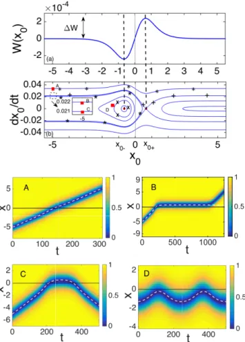
A. A single potential step
Our first scattering “experiment” refers to the case of a po-tential step only, corresponding toA >0andB = 0(cf. in-set I in Fig. 1). In this case, the effective potential has typically the form shown in the top panel of Fig. 5, while the associated phase-plane is shown in the middle panel of the same figure. Clearly, according to the particle picture for the soliton of the previous section, a dark soliton incident from the left towards the potential step can either be reflected or transmitted: if the soliton has a velocityv=dx0/dt, and thus a kinetic energy
K= 1 2v
2 =1
2sin 2
φ≈12φ2
, (25)
smaller (greater) than the effective potential step ∆W =
W(+∞)−W(−∞), as shown in the top panel of Fig. 5, then it will be reflected (transmitted). Notice the approximation (sinφ ≈ φ) here which is applicable for low speeds/kinetic energies. This consideration leads toφ < φc orφ > φc for
reflection or transmission, where the critical valueφc of the
soliton phase angle is given by:
φc = √
2∆W . (26)
In the numerical simulations, we found that the thresh-old between the two cases is quite sharp and is accurately predicted by Eq. (26). Indeed, consider the scenario shown in Fig. 5, corresponding to parameter values VL = 0,
VR = 0.01, αR = αL and µL = 1. In this case, we
find that∆W = 4.99×10⁻³
W(x
0
)
×10-3
-2 -1 0 1 2
x
0
-5 -3 -1 0 1 3 5
dx
0
/dt
-0.2 -0.1 0 0.1
-5 0.096
0.1
(b) (a)
A B
+
+ ∆W
*
*
*
*
*
+*
+ +FIG. 5: (Color online) The case of a single potential step,A= 0.01 andB = 0, corresponding toVL = 0,VR = 0.01,αR =αL, and µL= 1. Top panel (a): effective potentialW(x0); shown also is the
potential difference∆W =W(+∞)−W(−∞) = 4.99×10⁻³. Middle panel (b): corresponding phase plane; inset shows the initial conditions (red squares A and B) for the trajectories corresponding to reflection or transmission, while stars and crosses depict respec-tive PDE results. Bottom panel: contour plots showing the evolution of the dark soliton density for the initial conditions depicted in the middle panel, i.e.,x0=−5andφ= 9.6×10⁻²(left), orφ= 0.1
(right); note that, here,φc = 0.099. Thick (blue) solid lines show
PDE results, while dashed (white) lines depict ODE results.
x0 = −5, and for initial velocities corresponding to phase
angles φ = 9.6×10⁻²
orφ = 0.1, we observe reflection or transmission, respectively. The corresponding soliton tra-jectories are depicted both in the phase plane(x0, dx0/dt)in
the middle panel of Fig. 5 and in the space-time contour plots showing the evolution of the soliton density in the bottom pan-els of the same figure (see trajectories A and B for reflection and transmission, respectively). Note that stars and crosses in the middle panel correspond to results obtained by direct nu-merical integration of the partial differential equation (PDE), Eq. (5), while the (white) dashed lines in the bottom panels depict results obtained by the ordinary differential equation (ODE), Eq. (14). Obviously, the agreement between theoreti-cal predictions and numeritheoreti-cal results is very good.
Here we should recall that in the case where the nonlinear-ity step is also present (B 6= 0), and whenB > −A (for A >0) orB <−A(forA <0), the form of the effective po-tential is similar to the one shown in the top panel of Fig. 5. In such cases, corresponding results (not shown here) are qual-itatively similar to the ones presented above (forA 6= 0and B = 0); in addition, we have again captured accurately the velocity threshold for reflection/transmission.
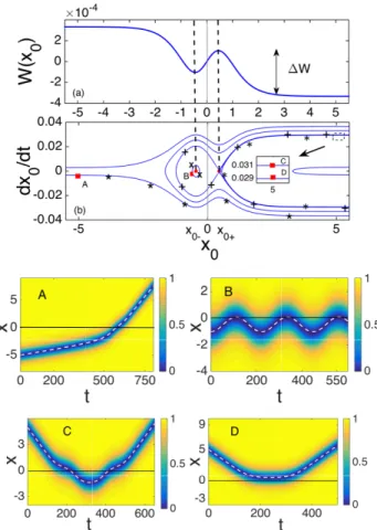
t
0 500 1000x
-9 -5 0 5 9
0 0.5 1 B
FIG. 6: (Color online) Similar to Fig. 5, but for a potential and a nonlinearity step,A = 0.01andB = −0.015, corresponding to
VL = 0, VR = 0.01, αR/αL = 0.985, andµL = 1. Top and
bottom panels show the effective potentialW(x0)and the associated
phase plane, respectively; the potential now features an elliptic and a hyperbolic fixed point atx0 ≈ ±0.65(cf. vertical dashed lines).
In the phase plane, initial conditions –marked with red squares– at pointsA(x0 = −5, φ = 0.034),B(x0 = −5, φ = 0.022),C
(x0 = −5, φ = 0.021) andD(x0 = −1.3, φ = 0.002) lead
to soliton transmission, quasi-trapping, reflection, and oscillations around the elliptic fixed point, respectively; asterisks, crosses and stars depict PDE results. The four bottom respective contour plots show the evolution of the soliton density; again, thick blue lines and white dashed lines depict PDE and ODE results, respectively.
B. A potential and a nonlinearity step
Next, we study the case where both a potential and a non-linearity step are present (i.e., A, B 6= 0), and there exist fixed points of the effective potential. One such case that we consider in more detail below is the one corresponding to A= 0.01andB =−0.015(respective parameter values are VL= 0,VR= 0.01,αR/αL = 0.985, andµL= 1). Note that
for this choice the effective potential asymptotically vanishes, as shown in the top panel of Fig. 6; nevertheless, results qual-itatively similar to the ones that we present below can also be obtained for nonvanishing asymptotics ofW(x0).
hyper-bolic fixed point, located atx0 ≈ ∓0.65respectively. In this
case too, one can identify an energy threshold∆W, now de-fined as∆W =W(x0+)−W(−∞) =W(x0+), needed to be
overcome by the soliton kinetic energy in order for the soliton to be transmitted (otherwise, i.e., forK <∆W, the soliton is reflected). Using the above parameter values, we find that
∆W = 2.4×10⁻⁴
and, hence, according to Eq. (26), the crit-ical phase angle for transmission/reflection isφc ≈0.022. In
the simulations, we considered a soliton with initial position and phase anglex0 =−5andφ= 0.034> φc, respectively
(cf. point A in the phase plane shown in the second panel of Fig. 6), and found that, indeed, the soliton is transmitted through the effective potential barrier of strength∆W. The respective trajectory (starting from point A) is shown in the second panel of Fig. 6. Stars along this trajectory, as well as contour plot A in the same figure, show PDE results obtained from direct numerical integration of Eq. (5); as in the case of Fig. 5, the (white) dashed line corresponds to the ODE result. To study the possibility of soliton trapping, we have also used an initial condition at the stable branch, incoming to-wards the hyperbolic fixed point, namely x0 = −5 and
φ =φc ≈0.022(point B in the second panel of Fig. 6). In
this case, the soliton reaches at the location of the hyperbolic fixed point (cf. incoming branch, marked with pluses) and ap-pears to be trapped at the saddle; however, this trapping occurs only for a finite time (fort≈600). At the PDE level, this can be understood by the the fact that such a configuration (i.e., a stationary dark soliton located at the hyperbolic fixed point) is unstable, as per the analysis of Sec. II.D. Then, the soliton es-capes and moves to the region ofx >0, following the trajec-tory marked with pluses forx > x0+(here, the pluses depict
the PDE results). The corresponding contour plot B, in the third panel of Fig. 6, shows the evolution of the dark soliton density. Note that, in this case, the result obtained by the ODE (cf. white dashed line) is only accurate up to the escape time, as small perturbations within the infinite-dimensional system destroy the delicate balance of the unstable fixed point.
For the same form of the effective potential, we have also used initial conditions that lead to soliton reflection. In partic-ular, we have again usedx0 = −5 andφ = 0.021 < φc,
as well as an initial soliton location closer to the potential and nonlinearity step, namelyx0 = −1.3, andφ = 0.002.
These initial conditions are respectively indicated by the (red) squares C and D in the second panel of Fig. 6. Relevant tra-jectories in the phase plane, as well as respective PDE results (cf. stars and X marks), can also be found in the same panel, while contour plots C and D in the bottom panel of Fig. 6 show the evolution of the soliton densities. It can readily be observed that for the slightly subcritical value of the phase angle (φ = 0.021), the soliton is again quasi-trapped at the hyperbolic fixed point, but for a significantly smaller time (for t ≈ 150). On the other hand, when the soliton is initially located closer to the steps and has a sufficiently small initial velocity, it performs oscillations, following the periodic orbit shown in the second panel of Fig. 6.
In all the above cases, we find a very good agreement be-tween the analytical predictions and the numerical results. Similar agreement was also found for other forms of the
ef-FIG. 7: (Color online) Similar to Fig. 6, for a potential and a nonlin-earity step, but now forA= 0.01andB =−0.017, corresponding toVL= 0,VR= 0.01,αR/αL= 0.983, andµL= 1. The effective
potentialW(x0) (top panel), exhibits an elliptic and a hyperbolic
fixed point, atx0± =±0.44(vertical dashed lines). In the
associ-ated phase plane (second panel) shown are initial conditions, for a soliton moving to the right, at points A (x0 =−5,φ= 0.005) and
B (x0=−1,φ= 0.001), as well as for a soliton moving to the left,
at points C (x0 = 5,φ = 0.031> φc ≈0.030) and D (x0 = 5, φ= 0.029< φc); in the relevant trajectories, stars, X marks, pluses
and asterisks, respectively, denote PDE results. Corresponding con-tour plots for the soliton density are shown in the bottom panels, with the dashed white lines depicting ODE results.
fective potential, as shown, e.g., in the example of Fig. 7 (see also inset III of Fig. 1). For this form ofW(x0),
parame-tersAandB areA = 0.01andB =−0.017(forVL = 0,
VR = 0.01,αR/αL = 0.983, andµL = 1), while there exist
again an elliptic and a hyperbolic fixed point, atx0±=±0.44
respectively. In such a situation, if a soliton moves from the left towards the potential and nonlinearity steps, and is placed sufficiently far from (close to) them – cf. initial condition at point A (point B) – then it will be transmitted (perform oscillations aroundx0−). On the other hand, if a soliton is
initially placed at somex0 > x0+ and moves to the left
to-wards the potential and nonlinearity steps, it faces an effec-tive barrier∆W (cf. top panel of Fig. 7), now defined as
∆W =W(x0+)−W(+∞). In this case too, choosing an an
towardsx0+, i.e., for the critical phase angleφc ≈0.03, it is
possible and achieve quasi-trapping of the soliton for a finite time, of the order oft ≈ 600. As such a situation was al-ready discussed above (cf. panel B of Fig. 6), here we present results pertaining to the slightly supecritical and subcritical cases, namelyφ = 0.031 > φc andφ = 0.029 < φc; cf.
(red) squares C and D in the second panel, and correspond-ing contour plots in the bottom panel of Fig. 7. It is readily observed that, in the former case, the soliton is initially trans-mitted through the interface; however, it then follows a trajec-tory surrounding the homoclinic orbit (see the orbit marked with plus symbols, which depicts the PDE results, in the sec-ond panel of Fig. 7), and is eventually reflected. In the case φ = 0.029 < φc, the soliton reachesx0+, stays there for a
timet ≈ 180, and eventually is reflected back following the trajectory marked with asterisks (see second panel of Fig. 7). In all cases pertaining to this form ofW(x0), the agreement
between the analytical predictions and the numerical results is very good as well.
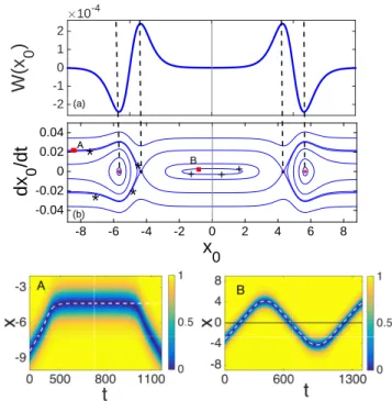
C. Rectangular barriers
Our analytical approximation can straightforwardly be ex-tended to the case of multiple potential and nonlinearity steps. Here, we will present results for such a case, where two steps, located atx= −Landx= L, are combined so as to form rectangular barriers, in both the linear potential and the non-linearity of the system. In particular, we consider the follow-ing profiles for the potential and the scatterfollow-ing length:
V(x) = Vb(x) +
(
VR, |x|> L
VL, |x|< L
, (27)
α(x) =
(
αR, |x|> L
αL, |x|< L
. (28)
In such a situation, the effective potential can be found fol-lowing the lines of the analysis presented in Sec. II.B: taking into regard that the perturbationP(υ)in Eq. (7) has now the form:
P(υ) = A+B|υ|2
υ[H(x+L)− H(x−L)],(29)
it is straightforward to find that the relevant effective potential is given by:
W(x0) = 1
8 2A+B
[tanh(L−x0) + tanh(L+x0)]
+ 1
24B[tanh 3
(L−x0) + tanh 3
(L+x0)]. (30)
Typically, i.e., for sufficiently large arbitrary values ofL, the effective potential is as shown in the top panel of Fig. 8; in this example, we used L = 5, while A = 0.01 and B = −0.015. It is readily observed that, in this case, asso-ciated with such a potential and a nonlinearity barrier, is an effective potential of the form of a superposition of the ones shown in Fig. 6, which are now located at±5. The associated
W(x
0
)
×10-4
-2 -1 0 1 2
x
0
-8 -6 -4 -2 0 2 4 6 8
dx
0
/dt
-0.04 -0.02 0 0.02 0.04
(a)
*
*
+
(b)
*
*
+ +FIG. 8: (Color online) The case of two potential and nonlinearity steps forming respective rectangular barriers, forL= 5,A= 0.01 andB =−0.015, corresponding toVL= 0,VR= 0.01,αR/αL=
0.985,µL = 1. Top panel (a): the effective potentialW(x0)[cf.
Eq. (30)], featuring elliptic fixed points at the origin and at±5.66, and a pair of hyperbolic fixed points at±4.34. Middle panel (b): the associated phase plane; (red) squaresAandBdepict different ini-tial conditions, corresponding to quasi-trapping or oscillations, while stars and crosses depict respective PDE results. Bottom panels: con-tour plots showing the evolution of the dark soliton density for the initial conditions depicted in the middle panel, i.e.,x0 =−8.6and φ= 2.2×10⁻²(left), orx0=−3andφ= 3×10⁻³(right); here, as before, dashed (white) lines depict ODE results.
phase plane is shown in the middle panel of Fig. 8; shown also are initial conditions corresponding to soliton quasi-trapping, or oscillations around the elliptic fixed point at the origin – cf. red square points A and B, respectively. The correspond-ing soliton trajectories are depicted both in the phase plane in the middle panel of Fig. 8 and in the space-time contour plots showing the evolution of the soliton density in the bot-tom panels of the same figure. Note that stars and plus sym-bols in the middle panel correspond to PDE results, obtained in the framework of Eq. (5), while the (white) dashed lines in the bottom panels depict ODE results, obtained by Eq. (14) for the potential in Eq. (30. Obviously, once again, agreement between theoretical predictions and numerical results is very good.
W(x
0
)
×10-4
0 10 20
x
0
-6 -4 -2 0 2 4 6
dx
0
/dt
-0.1 0 0.1
* *
* * * * ∆W
A
FIG. 9: (Color online) The case of two potential and nonlinearity steps forming respective rectangular barriers, forL= 0.1,A= 0.1 andB = −0.13, corresponding toaR/aL = 0.87,VR = 0.1and
µL = 1. Top panel: the effective potentialW(x0), featuring a
hy-perbolic fixed point at the origin and a pair of elliptic fixed points at±1.38. Middle panel: the associated phase plane; (red) squareA depicts an initial condition corresponding to quasi-trapping of the soliton, while stars depict respective PDE results. Bottom panel: contour plot showing the evolution of the dark soliton density for the initial condition depicted in the middle panel, i.e.,x0 =−5and φ= 5.8×10⁻²; as before, dashed (white) lines depict ODE results.
W(x0) = (b/4)sech 2
(x0). This result recovers the one
re-ported in Ref. [9] (see also Refs. [8, 10]), where the inter-action of dark solitons with localized impurities was studied; cf. Eq. (16) of that work, but in the absence of the trapping potentialUtr.
In the same limiting case of smallL, and forB 6= 0, the effective potential has typically the form shown in the top panel of Fig. 9; here, we useL = 0.1, while A = 0.1and B = −0.13, corresponding to aR/aL = 0.87, VR = 0.1
andµL = 1. Comparing this form ofW(x0) with the one
shown in Fig. 8, it becomes clear that as L → 0, the indi-vidual parts of the effective potential of Fig. 8 pertaining to the two potential/nonlinearity steps move towards the origin. There, they merge at the location of the “central” elliptic fixed point, which becomes unstable through a pitchfork bifurca-tion. As a result of this process, an unstable (hyperbolic) fixed point emerges at the origin, while the “outer” pair of the ellip-tic fixed points (cf. Fig. 8) also drift towards the origin – in this case, they are located at±1.38.
In the middle panel of Fig. 9, shown also is the phase plane associated to the effective potential of the top panel. As in the cases studied in the previous sections, we may investi-gate possible quasi-trapping of the soliton, using an initial
condition at the stable branch, incoming towards the hyper-bolic fixed point at the origin. Indeed, choosingx0=−5and
φ = φc = 5.8×10⁻² (notice that here, the corresponding
effective barrier∆W = 1.7×10⁻³– cf. top panel of Fig. 9),
we find the following: the soliton arrives at the origin, stays there for a timet ≈ 600, and then it is transmitted through the regionx >0. In fact, the corresponding trajectory found at the PDE level is depicted by stars in the middle panel of Fig. 9, while the relevant contour plot showing the evolution of the soliton density is shown in the bottom panel of the same figure. Notice, again, the fairly good agreement between nu-merical and analytical results.
We note that for the same parameter values, but forB= 0, elliptic fixed points do not exist, and the effective potential has simply the form of a sech2 barrier, as mentioned above
(see also work of Ref. [9]). In this case, starting from the same initial position,x0 =−5, and forφ= 0.1
(correspond-ing toφc = √
2∆W ≈0.1), we find that the trapping time is t≈320, i.e., almost half of the one that was when the nonlin-earity steps are present (results not shown here). This observa-tion, along with the results presented in the previous sections, indicate that nonlinearity steps/barriers are necessary either to facilitate or enhance soliton trapping in such inhomogeneous settings.
IV. DISCUSSION AND CONCLUSIONS
We have studied matter-wave dark solitons near linear tential and nonlinearity steps, superimposed on a box-like po-tential that was assumed to confine the atomic Bose-Einstein condensate. The formulation of the problem finds a direct application in the context of nonlinear optics: the pertinent model can be used to describe the evolution of beams, car-rying dark solitons, near interfaces separating optical media with different linear refractive indices and different defocus-ing Kerr nonlinearities.
Assuming that the potential/nonlinearity steps were small, we employed perturbation theory for dark solitons to show that, in the adiabatic approximation, solitons behave as equiv-alent particles moving in the presence of an effective poten-tial. The latter was found to exhibit various forms, ranging from simple tanh-shaped steps – for a spatially homogeneous scattering length (or same Kerr nonlinearity, in the context of optics) – to more complex forms, featuring hyperbolic and el-liptic fixed points – in the presence of steps in the scattering length (different Kerr nonlinearities).
corre-sponding numerical findings obtained in the framework of the BdG analysis.
We then studied systematically soliton dynamics, for a vari-ety of parameter values corresponding to all possible forms of the effective potential. Adopting the aforementioned equiv-alent particle picture, we found analytically necessary con-ditions for soliton reflection at, or transmission through the potential and nonlinearity steps: these correspond to initial soliton velocities smaller or greater to the energy of the effec-tive steps/barriers predicted by the perturbation theory and the equivalent particle picture.
We also investigated the possibility of soliton (quasi-) trap-ping, for initial conditions corresponding to the incoming, sta-ble manifolds of the hyperbolic fixed points (which exist only for inhomogeneous nonlinearities). In the context of optics, such a trapping can be regarded as the formation of surface dark solitons at the interface between dielectrics of different refractive indices. We found that trapping is possible, but only for a finite time. This effect can be understood by the fact that stationary solitons at the hyperbolic fixed points are unstable, as was corroborated by the BdG analysis. Thus small pertur-bations (at the PDE level) eventually cause the departure of the solitary wave from the relevant fixed points. Nevertheless, it should be pointed out that the time of soliton quasi-trapping was found to be of the order of600√2ξ/cSin physical units;
thus, typically, for a healing lengthξ of the order of a mi-cron and a speed of sound cs of the order of a
millimeter-per-second, trapping time may be of the order of≈850ms. This indicates that such a soliton quasi-trapping effect may be observed in real experiments. Note that in all scenarios (reflection, transmission, quasi-trapping) our analytical pre-dictions were found to be in very good agreement with direct numerical simulations in the framework of the original Gross-Pitaevskii model.
We have also extended our considerations to study cases involving two potential and nonlinearity steps, that are com-bined so as to form corresponding rectangular barriers. Re-flection, transmission and quasi-trapping of solitons in such cases were studied too, again with a very good agreement be-tween analytical and numerical results. In this setting, special attention was paid to the limiting case of infinitesimally small distance between the adjacent potential/nonlinearity steps that form the barriers. In this case, we found that, due to a pitch-fork bifurcation, the stability of the fixed point of the effective potential at the barrier center changes: out of two hyperbolic and one elliptic fixed point, a hyperbolic fixed point emerges, and the potential rectangular barrier is reduced to a delta-like
impurity. The latter is described by a sech2effective potential,
in accordance with the analysis of earlier works [8–10]. Our methodology and results pose a number of interesting questions for future studies. First, it would be interesting to investigate how our perturbative results change as the poten-tial/nonlinearity steps or barriers become larger, and/or attain more realistic shapes (including steps bearing finite widths, as well as Gaussian barriers – cf., e.g., recent work of Ref. [13]). In the same context, a systematic numerical – and, possibly, also analytical – study of the radiation of solitons during re-flection or transmission (along the lines, e.g., of Ref. [54]) should also provide a more complete picture in this prob-lem. Furthermore, a systematic study of settings involving multiple such steps/barriers, and an investigation of the pos-sibility of soliton trapping therein, would be particularly rele-vant. In such settings, investigation of the dynamics of mov-ing steps/barriers could find direct applications to fundamen-tal studies relevant, e.g., to superfluidity (see, for instance, Ref. [19]), transport of BECs [20], and even Hawking radia-tion in analog black hole lasers implemented with BECs [66]. Finally, extension of our analysis to higher-dimensional set-tings, would also be particularly challenging: first, in order to investigate transverse excitation effects that are not cap-tured within the quasi-1D setting, and second to study simi-lar problems with vortices and other vortex structures. See, e.g., Ref. [67] for a summary of relevant studies in higher-dimensional settings, and Ref. [68] for a recent example of manipulation/control of vortex patterns and their formation via Gaussian barriers, motivated by experimentally accessible laser beams.
Acknowledgments
The work of F.T. and D.J.F. was partially supported by the Special Account for Research Grants of the University of Athens. The work of F.T. and Z.A.A. was partially supported by Qatar University under the scope of the Internal Grant QUUG-CAS-DMSP-13/14-7. F.T. acknowledges hospitality at Qatar University, where most of this work was carried out. The work of P.G.K. at Los Alamos is partially supported by the US Department of Energy. P.G.K. also gratefully acknowl-edges the support of NSF-DMS-1312856, BSF-2010239, as well as from the US-AFOSR under grant FA9550-12-1- 0332, and the ERC under FP7, Marie Curie Actions, People, Inter-national Research Staff Exchange Scheme (IRSES-605096).
[1] Yu. S. Kivshar and B. A. Malomed, Rev. Mod. Phys. 61, 763 (1989).
[2] I. M. Lifshitz and A. M. Kosevich, Rep. Prog. Phys. 29, 217 (1966).
[3] I. Ianni, S. L. Coz, and J. Royer, arXiv:1506.03761. [4] A. M. Kosevich, Physica D 41, 253 (1990).
[5] X. D. Cao and B. A. Malomed, Phys. Lett. A 206, 177 (1995). [6] R. H. Goodman, P. J. Holmes, and M. I. Weinstein, Physica D
192, 215 (2004).
[7] J. Holmer, J. Marzuola, and M. Zworski, Comm. Math. Phys. 274, 187 (2007); J. Holmer, J. Marzuola, and M. Zworski, J. Nonlin. Sci. 17, 349 (2007).
[8] V. V. Konotop, V. M. P´erez-Garc´ıa, Y.-F. Tang, and L. V´azquez, Phys. Lett. A 236, 314 (1997).
(2002).
[10] N. Bilas and N. Pavloff, Phys. Rev. A 72, 033618 (2005). [11] N. Bilas and N. Pavloff, Phys. Rev. Lett. 95, 130403 (2005). [12] G. Herring, P. G. Kevrekidis, R. Carretero-Gonz´alez, B. A.
Mal-omed, D. J. Frantzeskakis, and A. R. Bishop, Phys. Lett. A 345, 144 (2005).
[13] I. Hans, J. Stockhofe, and P. Schmelcher, Phys. Rev. A 92, 013627 (2015).
[14] T. Ernst and J. Brand, Phys. Rev. A 81, 033614 (2010). [15] C. Lee and J. Brand, Europhys. Lett. 73, 321 (2006).
[16] J. L. Helm, T. P. Billam, and S. A. Gardiner, Phys. Rev. A 85, 053621 (2012).
[17] A. D. Martin and J. Ruostekoski, New J. Phys. 14, 043040 (2012).
[18] Y. Nogami and F. M. Toyama, Phys. Lett. A 184, 245-250 (1994).
[19] P. Engels and C. Atherton, Phys. Rev. Lett. 99, 160405 (2007). [20] D. Dries, S. E. Pollack, J. M. Hitchcock, and R. G. Hulet, Phys.
Rev. A 82, 033603 (2010).
[21] J. Cuevas, P. G. Kevrekidis, B. A. Malomed, P. Dyke, and R. G. Hulet, New J. Phys. 15, 063006 (2013).
[22] A. L. Marchant, T. P. Billam, T. P. Wiles, M. M. H. Yu, S. A. Gardiner, and S. L. Cornish, Nat. Com. 4, 1865 (2013). [23] V. Achilleos, P. G. Kevrekidis, V. M. Rothos, and D. J.
Frantzeskakis, Phys. Rev. A 84, 053626 (2011).
[24] A. ´Alvarez, J. Cuevas, F. R. Romero, C. Hamner, J. J. Chang, P. Engels, P. G. Kevrekidis, and D. J. Frantzeskakis, J. Phys. B: At. Mol. Opt. Phys. 46, 065302 (2013).
[25] G. Theocharis, P. Schmelcher, P. G. Kevrekidis, and D. J. Frantzeskakis, Phys. Rev. A 72, 033614 (2005).
[26] S. Middelkamp, P. G. Kevrekidis, D. J. Frantzeskakis and P. Schmelcher, Phys. Lett. A 373, 262268 (2009).
[27] Y. V. Kartashov, B. A. Malomed, and L. Torner, Rev. Mod. Phys. 83, 247 (2011).
[28] F. Kh. Abdullaev and M. Salerno, J. Phys. B: At. Mol. Opt. Phys. 36, 2851 (2003).
[29] M. I. Rodas-Verde, H. Michinel, and V. M. P´erez-Garc´ıa, Phys. Rev. Lett. 95, 153903 (2005); A. V. Carpentier, H. Michinel, M. I. Rodas-Verde, and V. M. P´erez-Garc´ıa, Phys. Rev. A 74, 013619 (2006).
[30] F. Tsitoura, P. Kr¨uger, P. G. Kevrekidis, and D. J. Frantzeskakis, Phys. Rev. A, 91, 033633 (2015).
[31] G. Theocharis, P. Schmelcher, P. G. Kevrekidis, and D. J. Frantzeskakis, Phys. Rev. A 74, 053614 (2006); J. Garnier and F. Kh. Abdullaev, ibid. 74, 013604 (2006); P. Niarchou, G. Theocharis, P. G. Kevrekidis, P. Schmelcher, and D. J. Frantzeskakis, ibid. 76, 023615 (2007).
[32] C. Wang, K.J.H. Law, P. G. Kevrekidis, and M. A. Porter, Phys. Rev. A 87, 023621 (2013).
[33] G. Dong, B. Hu, and W. Lu, Phys. Rev. A 74, 063601 (2006). [34] H. Sakaguchi and B. A. Malomed, Phys. Rev. A 81, 013624
(2010);
[35] S. Holmes, M. A. Porter, P. Kr¨uger, and P. G. Kevrekidis, Phys. Rev. A 88, 033627 (2013).
[36] K. Hizanidis, Y. Kominis, and N. K. Efremidis, Opt. Express 16, 18296 (2008).
[37] R. Marangell, C.K.R.T. Jones, and H. Susanto, Nonlinearity 23, 2059 (2010).
[38] R. Marangell, H. Susanto, and C.K.R.T. Jones, J. Diff. Eq. 253, 1191 (2012).
[39] C. Wang, P. G. Kevrekidis, T. P. Horikis, and D. J. Frantzeskakis, Phys. Lett. A 374, 3863 (2010); T. Mithun, K. Porsezian, and B. Dey, Phys. Rev. E 88, 012904 (2013). [40] F. Pinsker, N. G. Berloff, and V. M. P´erez-Garc´ıa, Phys. Rev. A
87, 053624 (2013).
[41] A. Balaz, R. Paun, A. I. Nicolin, S. Balasubramanian, and R. Ramaswamy, Phys. Rev. A 89, 023609 (2014).
[42] T. Kaneda and H. Saito, Phys. Rev. A 90, 053632 (2014). [43] A. Weller, J. P. Ronzheimer, C. Gross, J. Esteve, M. K.
Oberthaler, D. J. Frantzeskakis, G. Theocharis, and P. G. Kevrekidis, Phys. Rev. Lett. 101, 130401 (2008); S. Stellmer, P. Soltan-Panahi, S. D¨orscher, M. Baumert, E.-M. Richter, J. Kronj¨ager, K. Bongs, and K. Sengstock, Nat. Phys. 4, 496 (2008); S. Stellmer, C. Becker, P. Soltan-Panahi, E.-M. Richter, S. D¨orscher, M. Baumert, J. Kronj¨ager, K. Bongs, and K. Sen-gstock, Phys. Rev. Lett. 101, 120406 (2008); G. Theocharis, A. Weller, J. P. Ronzheimer, C. Gross, M. K. Oberthaler, P. G. Kevrekidis, and D. J. Frantzeskakis, Phys. Rev. A 81, 063604 (2010).
[44] B. T. Seaman, L. D. Carr, and M. J. Holland, Phys. Rev. A, 71, 033609 (2005).
[45] L. D. Carr, R. R. Miller, D. R. Bolton, and S. A. Strong, Phys. Rev. A 86, 023621 (2012).
[46] S. Inouye, M. R. Andrews, J. Stenger, H. J. Miesner, D. M. Stamper-Kurn, and W. Ketterle, Nature (London) 392, 151 (1998); J. Stenger, S. Inouye, M. R. Andrews, H.-J. Miesner, D. M. Stamper-Kurn, and W. Ketterle, Phys. Rev. Lett. 82, 2422 (1999); J. L. Roberts, N. R. Claussen, J. P. Burke, Jr., C. H. Greene, E. A. Cornell, and C. E.Wieman, ibid. 81, 5109 (1998); S. L. Cornish, N. R. Claussen, J. L. Roberts, E. A. Cornell, and C. E. Wieman, ibid. 85, 1795 (2000).
[47] F. K. Fatemi, K. M. Jones, and P. D. Lett, Phys. Rev. Lett. 85, 4462 (2000); M. Theis, G. Thalhammer, K. Winkler, M. Hell-wig, G. Ruff, R. Grimm, and J. H. Denschlag, ibid. 93, 123001 (2004).
[48] A. C. Newell and J. V. Moloney, Nonlinear Optics (Addison-Wesley, Redwood City, CA, 1992).
[49] A. B. Aceves, J. V. Moloney, and A. C. Newell, J. Opt. Soc. Am. B 5, 559 (1988); Phys. Lett. A 129, 231 (1988); Phys. Rev. A 39, 1809 (1989); ibid. 39, 1828 (1989).
[50] Yu. S. Kivshar, A. M. Kosevich, and O. A. Chubykalo, Phys. Rev. A 41, 1677 (1990).
[51] Yu. S. Kivshar and M. L. Quiroga-Texeiro, Phys. Rev. A 48, 4750 (1993).
[52] Y. Kominis and K. Hizanidis, Phys. Rev. Lett. 102, 133903 (2009).
[53] H. Sakaguchi and M. Tamura, J. Phys. Soc. Jpn. 74, 292 (2005). [54] N. G. Parker, N. P. Proukakis, M. Leadbeater, and C. S. Adams,
J. Phys. B: At. Mol. Opt. Phys. 36 2891 (2003).
[55] N. P. Proukakis, N. G. Parker, D. J. Frantzeskakis, and C. S. Adams, J. Opt. B: Quantum Semiclass. Opt. 6, S380 (2004). [56] H. Sakaguchi, Laser Phys. 16, 340 (2006).
[57] L. P. Pitaevskii and S. Stringari, Bose-Einstein Condensation (Oxford University Press, Oxford, 2003).
[58] P. G. Kevrekidis, D. J. Frantzeskakis, and R. Carretero-Gonz´alez (eds.), Emergent Nonlinear Phenomena in Bose-Einstein Condensates: Theory and Experiment (Springer-Verlag, Berlin, 2008); R. Carretero-Gonz´alez, D. J. Frantzeskakis, and P. G. Kevrekidis, Nonlinearity 21, 139 (2008).
[59] R. Folman, P. Kr¨uger, J. Denschlag, J. Schmiedmayer, and C. Henkel, Adv. At. Mol. Opt. Phys. 48, 263 (2002).
[60] L. D. Carr, C. W. Clark, and W. P. Reinhardt, Phys. Rev. A 62, 063610 (2000).
[61] Yu. S. Kivshar and X. Yang, Phys. Rev. E 49, 1657 (1994). [62] D. J. Frantzeskakis, J. Phys. A: Math. Theor. 43, 213001 (2010). [63] M. J. Ablowitz, S. D. Nixon, T. P. Horikis, and D. J.
[64] D. E. Pelinovsky and P. G. Kevrekidis, ZAMP 59, 559 (2008). [65] A. S. Rodrigues, P. G. Kevrekidis, Mason A. Porter, D. J.
Frantzeskakis, P. Schmelcher, and A. R. Bishop, Phys. Rev. A 78, 013611 (2008).
[66] J. Steinhauer, Nat. Phys. 10, 864 (2014).
[67] P. G. Kevrekidis, D. J. Frantzeskakis, and R.
Carretero-Gonz´alez, The defocusing Nonlinear Schr¨odinger Equation: From Dark Solitons to Vortices and Vortex Rings (SIAM, Philadelphia, 2015).
![FIG. 3: (Color online) Same as Fig. 2, but for a soliton located at the elliptic fixed point x 0− = −0.66; this state is found using the initial ansatz υ s (x) = [1 − V (x)] 1 /2 tanh(x + 0.2)](https://thumb-us.123doks.com/thumbv2/123dok_us/8274792.2191470/5.918.524.781.78.632/color-online-soliton-located-elliptic-using-initial-ansatz.webp)