Vol 60, No 4 (2017)

(1)

TECHNICAL UNIVERSITY OF CLUJ-NAPOCA

ACTA TECHNICA NAPOCENSIS

Series: Applied Mathematics, Mechanics, and Engineering Vol. 60, Issue IV, November, 2017

MOBILE CAM MECHANISMS SYNTHESIS USING THE

CHARACTERISTIC POINTS. PART II: APPLICATIONS

Claudia-Mari POPA, Dinel POPA, Nicolae-Doru STĂNESCU, Nicolae PANDREA

Abstract: The paper is a continuation of the previous paper in which are presented simple mechanisms and mobile cam complex mechanisms. Based on the working algorithm established in the previous paper, the present paper presents an AutoLisp function which, in three applications, produces the cams of simple mechanisms and of mobile cam complex mechanisms. For each case are determined the errors in obtaining the cam profile depending on the number of characteristic points used. At the end of the paper the advantages of this method are presented.

Key words: Mechanism, cam, follower, synthesis, characteristic points, function, AutoLisp, AutoCAD.

1. INTRODUCRTION

In the first part of the paper ([8]) were classified the mobile cam mechanisms and were presented examples of complex cam mechanisms and their field of use. A calculation algorithms was also presented for a graphical synthesis method, method that is based on the characteristic points with AutoLisp functions. The second part of the paper, the current one, presents 3 applications for simple and complex mechanisms with mobile cam based on the algorithm established in the first part.

2. APPLICATIONS

2.1. Mechanism with rotational cam and flat oscillating follower

The kinematic scheme of a flat mechanism with rotational cam and flat oscillating follower is given in Fig. 1.

One knows:

– the coordinates in mm of points O₁(0,0)

and O₂(30,20);

– the lengths: O₂M = r₀ = 5mm,

mm 50 = = l

MN ,

– displacement's law of the follower:

x

y

1

x2

ϕ

θ

O (X ,Y ) M

N X

Y

2 2 2

O (X ,Y )₁ 1 1

y₂

Fig. 1. Mechanism with rotation cam and oscillating follower.

β − α =

θ , (`)

where

ϕ +

ϕ −

=

α −

sin cos tan

2 2 1

e X

e Y

, ₍₂₎

2 0 2

0 1

) (

tan

r R d

r R

+ −

+ =

β − _,

(3)

(

)

(

)

2

2 2

2 + sinϕ + − cosϕ

= X e Y e

d . (4)

In the previous relations R =10mmand mm

5 =

e .

The cam groove is required.

(2)

values of the cam groove and in a script file with the building instructions of the cam groove. In this way, we will have both a graphical image of the consecutive positions of the follower and the construction of the cam, that certifies the correctness of the method.

The content of the AutoLisp function called

Cam is the following:

(Defun C:Cam () (Data)

(Initialization) (Opening_Files)

(Calculation_Constants) (Setq phi 0)

(While (< phi 360) (Calculations) (Memoration_Ci) (Setq phi(+ phi step)) (Calculations)

(Drawing_Ciplus1) (Memoration_Ciplus1) (Coordinates_Ai) (Writing_Files) )

(Closing_Files) )

The AutoLisp function is called in AutoCAD. In turn it calls other AutoLisp functions or AutoCAD commands.

The first function that is called is Data and has the following content:

(Defun Data ()

(Setq X1 0.0 Y1 0.0 X2 30.0 Y2 20.0 RCapital 10.0 r0 5.0 esmall 5.0 lsmall 50.0 step 0.1) )

With the multiple assignment function Setq values are attributed to the coordinates of points

) , ( ₁ ₁

1 X Y

O , O₂(X₂,Y₂) as well to the other constructive dimensions.

The function has no parameters or local variables. By step is denoted the angular step

ϕ ∆ .

The second function that is called is

Initialization and has the following content:

(Defun Initialization ()

(Command "ERASE" "All" "" "OSNAP" "OFF" "ORTHO" "OFF")

(Command "ZOOM" "W" "-100,-100" "100,100")

)

This one calls the AutoLisp function

Command AutoCAD commands that erase the printed screen (ERASE), deactivates the

OSNAP and ORTHO modes and establish the dimensions of the viewing window (ZOOM).

The next function that is called is

Opening_Files with the following content:

(Defun Opening_Files ()

(Setq Draw(Open "Cama_01.scr" "W") Values(Open "Values_01.txt" "W")) (Write-Line "PLINE" Draw)

)

The function opens at writing, in the current folder, a script file and a text file. In the script file it will be written on the first command line

the AutoCAD command PLINE, instruction

that will materialize the cam.

In the function Calculation_Constants it is determined the distance O₁O₂ and the angle made by it with the horizontal.

(Defun Calculation_Constants ()

(Setq O1O2 (Distance (List X2 Y2) List X1 Y1)))

(Setq Phi0_rad (ATAN (/ Y2 x2)) Phi0_deg (* Phi0_rad (/ 180 PI)))

)

The AutoLisp, as any programming

language, operates with angles in radians and the graphical constructions in AutoCAD are made by specifying the angle in degrees. That's why the values of the angles are determined both in radians and degrees.

Continuing the function Cam, into a

repetitive cycle while, values are attributed to the angle ϕ (Phi) in the interval

[

0...360°

]

, starting from 0 (Setq Phi 0) with an angular step of ∆ϕ = step.

(3)

to the angle ϕ, the coordinates of point O₂( )i after the rotation with the angle ϕ₁( )i , the coordinates of points M and N from the bottom of the follower.

(Defun Calculations ()

(Setq phi_rad(* phi (/ Pi 180)))

(Setq Sup(- Y2 (* esmall Cos phi_rad)) Inf(+ X2 (* esmall Sin phi_rad))))

(Setq Alpha_rad(ATAN (/ Sup Inf)) Alpha_Deg(* Alpha_Rad (/ 180 Pi)))

(Setq dsmall(Sqrt(+ (* Inf Inf) (* Sup Sup)))) (Setq sum(+ RCapital r0) num(Sqrt(- (* dsmall dsmall) * sum sum))) beta_rad(ATAN(/ sum num)) beta_deg(* beta_rad (/ 180 Pi)))

(If (= phi 0)

(Setq Theta0_deg(- Alpha_deg beta_deg)) )

(Setq Theta_deg(- Alpha_deg beta_deg theta0_deg))

(Setq Rotation_deg(- Theta_deg phi) Rotation_rad(* Rotation_deg (/ Pi 180))) (Setq XO2(* O1O2 (Cos(- phi0_rad phi_rad))) YO2(* O1O2 (Sin(- phi0_rad phi_rad))) Pct_O2(List XO2 YO2))

(Setq XN(- XO2 lsmall) YN(- YO2 r0) XM XO2 YM(- YO2 r0))

(Setq Pct_N (List XN YN) Pct_M (List XM YM))

(Setq Pct_N_Rotated(Polar Pct_O2 (+ (Angle Pct_O2 Pct_N) Rotation_rad) Distance Pct_O2 Pct_N)))

(Setq Pct_M_Rotated(Polar Pct_O2 (+ (Angle PCT_O2 Pct_M) Rotation_rad) (Distance Pct_O2 Pct_M)))

)

Saving the current position of the follower is done with the function Memoration_Ci:

(Defun Memoration_Ci ()

(Setq N_old Pct_N_Rotated M_old Pct_M_Rotated)

)

One continues to the next step ϕ = ϕ+∆ϕ (Setq + phi step) and is determined the new position of the follower with the same function

Calculations.

The function Drawing_Ciplus1 contains the plotting instructions in AutoCAD of a poly-line between the points O(i `1)MN

2

+ _{giving the}

position of the follower.

(Defun Drawing_Ciplus1 ()

(Command "PLine" Pct_N_Rotated Pct_M_Rotated "")

)

The coordinates of points M and N are saved with the function Memoration_Ciplus1.

(Defun Memorare_Ciplus1 ()

(Setq N_new Pct_N_Rotated M_new Pct_M_Rotated)

)

The coordinates of the characteristic point

i

A as intersection of two consecutive positions of the follower are determined with the function

Coordinates_Ai.

(Defun Coordinates_Ai ()

(Setq Pct_A(Inters N_old M_old N_new M_new Nil))

(Setq xA(princ(car Pct_A)) yA(princ(car(cdr Pct_A)))) )

With the function Inters it is determined the intersection point of the segments MN at every two steps i and i +1. The function analyzes two straight lines through their end points and returns, if exists, their intersection point.

The obtained values are written in a file with the function Writing_Files.

(Defun Writing_Files ()

(Setq text1(Strcat (rtos xA 2 6) "," (Rtos yA 2 6)) text2(Strcat (rtos phi 2 6) "," (rtos xA 2 6) "," (Rtos yA 2 6)))

(Write-Line text2 Values) (Write-Line text1 Draw) )

After closing the repetitive cycle, the opened files are also closed with the function

(4)

(Defun Closing_Files () (Write-Line "C" Draw) (Close Values)

(Close Draw) )

The AutoLisp function Cam that is

presented was made so that it can be used for any mechanism with rotation cam. Only the functions from inside of it will be modified, the structure remaining always the same.

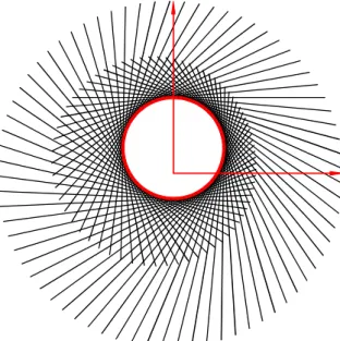
After calling it in AutoCAD the following construction captured in Fig. 2 will appear.

Fig. 2. The cam and the consecutive positions of the follower.

To grasp the consecutive positions of the follower for this construction, an angular step of5 was used. The cam obtain in the file ° cam_01.scr was represented with a bold line.

The relations (1) – (4) used for the displacement law of the follower are leading to obtaining a circle of radius R with the center at the point O(0,e). For determining the accuracy of the method we will call the function for an angular step of: 1°, ₀_.₂0_and₀_.₁0_{and we will}

determine the aria and perimeter of the closed poly-line (the cam) with the AutoCAD function

AREA.

For an angular step of 1 (360 positions) the ° following area is obtained _A ₌₃₁₄_.₁₆₇₅_mm2

and the perimeter P = 62.8335mm.

For an angular step of ₀_.₂0_{(1800 positions)}

the following area is obtained

2

mm 1596 . 314 =

A and the perimeter

mm 8319 . 62 =

P .

For an angular step of ₀_.₁0_{(3600 positions)}

the following area is obtained

2

mm 1593 . 314 =

A and the perimeter

mm 8319 . 62 =

P .

For a circle of radius R =10mm the area is

2

mm 1593 . 314 =

A and the perimeter

mm 8319 . 62 =

P . It is noted that for the 3600

positions of the follower are obtained the same values as in the case of theoretical cam. For 360 positions of the follower, the determining error of the groove is 0.0025%.

2.2. Mechanism with rotational cam and oscillating curved follower

In Fig. 3 is presented the kinematic scheme of the mechanism with rotational cam and oscillating curved follower.

1 1 1

O (X ,Y ) Y

X

θ

2 2

y

x

1 1

y x

O (X ,Y )₂ ₂ ₂

ϕ

Fig. 3. Mechanism with rotation cam and oscillating curved follower.

One knows:

– the coordinates in mm of points O₁(0,0)

and O₂(30,20)

– the distance O₂C = l = 30mm,

– the curvature radius of the follower mm

5

0 =

r ,

– the displacement law of the follower β

− α =

θ , (5)

where:

ϕ +

ϕ −

=

α −

sin cos tan

2 2 1

e X

e Y

(6)

a a2 1 1

tan −

=

(5)

(

)

(

)

(

)

, 2

2

sin sin

2 0 2

2 2

dl r R l

dl e Y e

X a

− − +

ϕ −

+ ϕ +

=

(8)

(

)

(

)

2

2 2

2 + sinϕ + − cosϕ

= X e Y e

d . (9)

In the previous relations R =10mm and mm

5 =

e . It is asked, as previously, the cam's

groove.

It is used the same AutoLisp Function Cam where will be modified just some of the functions from its body. Those functions are:

(Defun Data ()

(Setq X1 0.0 Y1 0.0 X2 30.0 Y2 20.0 RCapital 10.0 r0 5.0 esmall 5.0 lsmall 30.0 step 10) )

(Defun Calculation_Constants ()

(Setq O1O2 (Distance (List X2 Y2) (List X1 Y1)))

(Setq Phi0_rad (ATAN (/ Y2 x2)) Phi0_deg (* Phi0_rad (/ 180 PI)))

)

(Setq Sup(- Y2 (* esmall (Cos phi_rad))) Inf(+ X2 (* esmall (Sin phi_rad))))

(Setq Alpha_rad(ATAN (/ Sup Inf)) Alpha_Deg(* Alpha_Rad (/ 180 Pi)))

(Setq dsmall(Sqrt(+ (* Inf Inf) (* Sup Sup)))) (Setq sum(+ RCapital r0) asmall(/ (+ (* dsmall dsmall) (* lsmall lsmall) (* -1 sum sum)) 2.0 dsmall lsmall))

(Setq num(Sqrt(- 1.0 (* asmall asmall))) beta_rad(ATAN(/ num asmall)) beta_deg(* beta_rad (/ 180 Pi)))

(If (= phi 0)

(Setq Theta0_deg(- Alpha_deg beta_deg))) (Setq Theta_deg(- Alpha_deg beta_deg theta0_deg))

(Setq Rotation_deg(- Theta_deg phi) Rotation_rad(* Rotation_deg (/ Pi 180))) (Setq XO2(* O1O2 (Cos(- phi0_rad phi_rad))) YO2(* O1O2 (Sin(- phi0_rad phi_rad))) Pct_O2(List XO2 YO2))

(Setq XC(- XO2 lsmall) YC YO2 Pct_C(List XC YC) XB(+ XC r0) YB YO2 Pct_B(List XB YB) XD(- XC r0) YD YO2 Pct_D(List XD YD))

(Setq Pct_Br(Polar Pct_O2 (+ (Angle Pct_O2 Pct_B) Rotation_rad) (Distance Pct_O2 Pct_B)) Pct_Cr(Polar Pct_O2 (+ (Angle Pct_O2 Pct_C) Rotation_rad) (Distance Pct_O2 Pct_C)) Pct_Dr(Polar Pct_O2 (+ (Angle Pct_O2 Pct_D) Rotation_rad) (Distance Pct_O2 Pct_D)))

)

(Setq B_old Pct_Br C_old Pct_Cr D_old PCT_Dr)

)

(Defun Drawing_Ciplus1 ()

(Command "PLine" Pct_Dr "A" "CE" Pct_Cr Pct_Br "L" Pct_O2 "")

)

(Defun Memoration_Ciplus1 ()

(Setq B_new Pct_Br C_new Pct_Cr D_new Pct_Dr)

)

(Defun Coordinates_Ai () (setq a1(princ(car C_old))) (setq b1(princ(car(cdr C_old)))) (setq a2(princ(car C_new))) (setq b2(princ(car(cdr C_new)))) (Setq R1 r0 R2 r0)

(Int_2C)

(setq xA xP2 yA yP2) )

For determining the intersection points of two circles (the characteristic points A_i) a custom AutoLisp function was used named

Int_2C described in [7]. The function determines the intersection points of the circles centered at C₁(a₁,b₁), C₂(a₂,b₂) and of radii

1

R and R₂. The retrieved points are

) , ( ₁ ₁

1 xP yP

P and P₂(xP₂,yP₂). In the case where the circles are intersected in two points, the more convenient solution should be picked. In this case we chose the point P₂.

(6)

step of 10 . The cam was represented with a ° bold line.

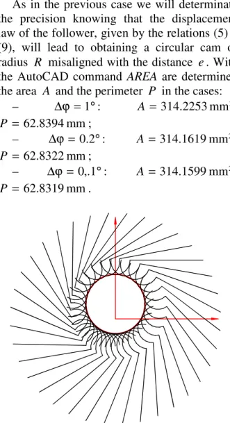
As in the previous case we will determinate the precision knowing that the displacement law of the follower, given by the relations (5) – (9), will lead to obtaining a circular cam of radius R misaligned with the distance e. With the AutoCAD command AREA are determined the area A and the perimeter P in the cases:

– ∆ϕ =1 : ° _A ₌ ₃₁₄_.₂₂₅₃_mm2_,

mm 8394 . 62 = P ;

– ∆ϕ = 0.2°: _A ₌ ₃₁₄_.₁₆₁₉_mm2_,

mm 8322 . 62 = P ;

– ∆ϕ = 0,.1°: _A ₌ ₃₁₄_.₁₅₉₉_mm2_,

mm 8319 . 62 = P .

Fig. 4. The cam and the consecutive positions of the follower.

We calculate the determination error of the external groove for 360 positions of the follower (∆ϕ =1 ) and then is obtained the ° value 0.012%.

In both applications the geometrical

constructions in 3600 positions (∆ϕ = 0.1°) will conduct to obtaining the exact solution.

2.3. Complex mechanism with rotation cam and curved follower in parallel-plane movement

For the complex mechanism with mobile cam from Fig. 5 there are known:

– the coordinates in mm of points O(0,0) and C(0,60),

– the lengths of the articulated four-bar

mechanism: OA = 20mm, AB = 60mm,

mm 60 =

BC ,

– cam base circle radius r₀ = 20mm and the curvature radius of the follower R =100mm,

– the displacement law of the element OA

) cos 1 ( 6 10

1 − ϕ

π + ϕ =

ϕ , (10)

where ϕ₁₀ = 60°. It is asked the cam groove.

O A B C 1 1 X Y x x2 y y₂

r O1 0 ϕ ϕ 1 ϕ2 R

Fig. 5. Complex mechanism with rotation cam and follower in parallel-plane movement.

There are chosen three coordinates systems:

XOY – the fixed coordinates system, x₁O₁y₁ – the mobile coordinates system rigidly jointed to the cam, and x₂Ay₂ – the mobile coordinates system rigidly jointed to the follower AB.

In the local reference system, the point O₂, the curvature center of the follower has the following coordinates:       − = = , 4 , 2 2 2 2 2 AB R yO AB xO (11)

and in the general reference system:

      ϕ + ϕ + ϕ = ϕ − ϕ + ϕ = . cos sin sin , sin cos cos 2 2 2 2 1 2 2 2 2 2 1 2 yO xO OA YO yO xO OA XO (12)

(7)

– determining the position of point A by knowing the length of the segment OA and of the angle ϕ₁₀,

– determining the coordinates of point B as the intersection of the circle of radius AB and center A with the circle of radius BC and center C; it will be chosen one of the intersection points (the one that is convenient),

– determining the angle ϕ₂ that the segment

AB is making with the horizontal,

– determining with the relations (11) and (12) the coordinates of point O₂ in the general reference system,

– determining the coordinates of point O₁ by

knowing the length of the segment

0 1

2O R r

O = + and the angle made by it with

the horizontal

2 3

2

π +

ϕ .

The algorithm from above was made for AutoLisp, a programming language that is vector one.

Next, for applying the method of

characteristic points and the AutoLisp function

Cam, we will have to proceed as follows: 1. the coordinate system is translated to point O₁ that was previously determined,

2. the coordinates of points O, A, B and C are obtained in the new coordinates system.

For determining a characteristic point A_i the following steps are needed:

3. the mechanism OABC is rotated with the angle ϕ around the point O₁,

4. the coordinates of points O, A, B and C are obtained in the new coordinates system,

5. the value of angle ϕ₁ is calculated with the relation (10),

6. the element OA is rotated towards the point O with the angle ϕ−ϕ₁ −ϕ₁₀,

7. the coordinates of point B are determined as an intersection of two circles,

8. in this position are determined the coordinates of point O₂( )i , the curvature center of the follower,

9. it is remembered the value of the coordinates of point O₂( )i ,

10. it is passed to the angle ϕ+ ∆ϕ,

11. the steps 3÷7 are repeated for this new angle,

12. in this position are determined the coordinates of point O₂(i+1), the curvature center of the follower,

13. it is remembered the value of the coordinates of point ( 1)

2

+ i

O ,

14. the characteristic point Ai is obtained as

an intersection point between the circles of radius R and centers O₂( )i and O₂(i+1),

15. we save the coordinates of point A_i. The previous algorithm permits an easy way to obtain AutoLisp functions in AutoCAD, by using the same AutoLisp function called Cam that is used at applications 2.1. and 2.2. The only things that will differ will be the functions from its body. Their content of their listing is the following:

(Setq phi1_rad(* (/ Pi 6) (- 1 (Cos (* phi (/ Pi 180))))))

(Setq ACapital(Polar OCapital (- phi_rad phi1_rad phi10_rad) OA) xA(princ(car ACapital)) yA(princ(car(cdr ACapital))) a1 xA b1 yA R1 AB a2 xC b2 yC R2 BC)

(Int_2C)

(Setq BCapital P1 xB xP1 yB yP1)

(Setq phi2_rad(Angle ACapital BCapital)) (Setq xsmallO2 (/ AB 2.0) ysmallO2 (Sqrt (- (* RCapital RCapital) (* 0.25 AB AB))))

(Setq XCapitalO2(+ xA (* xsmallO2 (Cos phi2_rad)) (* -1 ysmallO2 (Sin phi2_rad))) YCapitalO2(+ yA (* xsmallO2 (Sin phi2_rad)) (* ysmallO2 (Cos phi2_rad))))

)

(Defun Data ()

(Setq XO 0.0 YO 0.0 RCapital 100.0 r0 20.0 OA 20.0 AB 60.0 BC 60.0 xC 60.0 yC 0.0 phi10_deg 60.0 step 10)

)

(Defun Actualization ()

(8)

)

(Defun Calculation_Constants () (Setq phi 0 Phi_rad(* phi (/ Pi 180)))

(Setq OCapital(List XO YO) phi10_rad(* phi10_deg (/ Pi 180)))

(Calculations)

(Setq OCapital1(Polar (List XCapitalO2 YCapitalO2) (+ phi2_rad (* 3 (/ Pi 2))) (+ RCapital r0)) xO1(princ(car OCapital1)) yO1(princ(car(cdr OCapital1))))

(Setq Ung_O1O(Angle (List xO1 yO1) (List xO yO)) Ung_O1C(Angle (List xO1 yO1) (List xC yC)) Dist_O1O(Distance (List xO1 yO1) (List xO yO)) Dist_O1C(Distance (List xO1 yO1) (List xC yC)))

(Setq xOt(- XO xO1) yOt(- YO yO1) OCapital(List xOt yOt) xCt(- XC xO1) yCt(- YC yO1) CCapital(List xCt yCt) xAt(- XA xO1) yAt(- YA yO1) ACapital(List xAt yAt) xBt(- XB xO1) yBt(- YB yO1) BCapital(List xBt yBt) xO2t(- XCapitalO2 xO1) yO2t (- YCapitalO2 yO1) O2Capital (List xO2t yO2t))

)

(Setq XO2_old XCapitalO2 YO2_old YCapitalO2)

)

(Defun Drawing_Ciplus1 ()

(Command "Arc" "C" (List XCapitalO2 YCapitalO2) ACapital BCapital) (Command "Pline" OCapital ACapital BCapital "")

)

(Defun Memoration_Ciplus1 ()

(Setq XO2_new XCapitalO2 YO2_new YCapitalO2)

)

(Defun Coordinates_Ai ()

(Setq a1 XO2_old b1 YO2_old R1 RCapital a2 XO2_new b2 YO2_new R2 RCapital)

(Int_2C)

(Setq xI xP1 yI yP1) )

Same as in the case of application from point 2.2. it was used the AutoLisp function called

Int_2C.

It was used for determining the coordinates of point B, of the articulated four-bar mechanism, when the coordinates of points O

and C are varying for determining the

intersection points A_i.

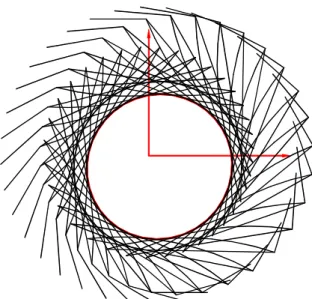
In Fig. 6 the mechanism was presented in 36 positions (with an angular step of 10 ) and also ° the cam for this construction.

Fig. 6. The cam and the consecutive positions of the mechanism.

In [1] it was made the analytical synthesis of the mechanism, the results being obtained by

following a Pascal based programming

language. The external groove was obtained by 360 points. Comparing the results by both methods and having as mark the external length of the groove, we obtain:

– the cam obtained by analytical method in 360 points: perimeter P =161.9712mm,

– the cam obtain by using the characteristic

points method in 360 positions:

mm 8836 . 161 =

P , in 1800 positions:

mm 8781 . 161 =

P and in 3600 positions:

mm 8779 . 161 =

P .

(9)

are increased the number of characteristic points.

6. CONCLUSIONS

The characteristic points method presented in the paper allows solving some problems that have graphical representation. The method, in the presence of a CAD software, is quick and precise and does not necessitates any complicated fundamental knowledge.

The AutoLisp functions presented in the 3 examples are general can be applied in the case of other cam mechanisms, in both synthesis or cinematic analysis. For instance, for the synthesis of the cam mechanism with triad in [8] (Fig. 7), mechanism at which one knows the dimensions of the elements, the positions of the kinematic pairs at the base and the law of motion of the element 5, ϕ₅

( )

ϕ , with

] 360 ... 0

[ °

∈

ϕ (ϕ being the rotational angle of

the cam 1), the working algorithm is:

1 2

O A B

E

4

5

C D

3 ₆

F G

H

Fig. 7. Mobile cam mechanism amplified with a triad.

1. one chooses a reference system in the rotational center O(0,0) of the cam;

2. relative to this reference frame one determines the coordinates of the kinematic pairs at base B, F and H;

For the position ϕ = 0 one determines: °

3. position of the mechanism FEGH

exactly as at the four-bar mechanism OABC in the application 2.3;

4. knowing the dimensions of the triangle

DEG one determines the position of point D; 5. position of the dyad DEB by intersecting a circle with the center at D and radius DC with a circle of radius BC at center at point C;

6. construction of the follower 2 and memorization of its position (curve C_i);

7. rotation of the mechanism BCDEFGH around point O with the angle ϕ+∆ϕ; it result the new position of the kinematic pairs at base;

8. one calculates the angle ϕ₅

( )

ϕ ;

9. rotation of the element 5 with the angle

50 5 −ϕ

ϕ −

ϕ ;

10. one repeats the steps 3–6 for this new angle and obtains the new position of the follower (curve C_i₊₁);

11. one obtains the characteristic point A_i as the intersection of two straight lines, like in application 2.1;

12. one puts into memory the coordinates of the point A_i.

The algorithm is similar to those in the previous applications. One also uses the AutoLisp program Cam and updates only the

functions Data, Calculations and

Calculation_Constants, the rest being those used in application 2.1. One also uses the function Int_2C to determine the intersection points of two circles, like in applications 2.2 and 2.3.

Regarding the precision in determining the cam groove, in the paper were used examples to which the solution was known. Comparing the results obtained for more positions of the follower it was concluded that for 3600 positions the solution is extremely precise.

In AutoCAD it is easy to determinate the length of a curve in a high number of points. For example at application 2.2, the length of the external groove of the circular cam was obtained in 36000 positions (with the angular step of ∆ϕ = 0.01°) and the area and

perimeter are: _A ₌ ₃₁₄_.₁₅₉₂₇₁_mm2_,

mm 831855 .

62 =

P . The AutoLisp function

(10)

REFERENCES

[1] Popa. D., Pandrea. N., Pandrea. M., Popa. C-M, Synthesis of the complex mechanisms

with mobile cam, ID: 594, 12th IFToMM

World Congress, Besançon (France),

June18-21, 2007.

[2] Artobolevski, I., Les mecanismes dans la

technique moderne, Tome 1-5, Ed. MIR, Moskow, 1978.

[3] Artobolevski, I. MECHANISMS in modern

Engineering Design. Vol. 1-5, Ed. MIR, Moskow, 1978.

[4] Scater, N., Mechanisms and mechanical

devices sourcebook, Fifth Edition, Mc Graw-Hill, 2011.

[5] Charles, W., Sadler P., Kinematics and

dynamics of machinery, Second Edition, Harper Collins College Publishers, 1993. [6] Norton, R.L., Design of Machinery: An

Introduction to the Synthesis and Analysis of Mechanisms and Machines, McGraw-Hill, 2003.

[7] Scater, N., Mechanisms and Mechanical

Devices, McGraw-Hill, 2011.

[8] Popa, C-M., Popa, D., Stănescu N-D, Pandrea, N., Mobile cam mechanisms using

the characteristic points, Part I: Theoretical notions and calculation algorithms, Acta

Technica Napocensis, Series: Applied

Mathematics, Mechanics, and Engineering, Technical University of Cluj-Napoca.

SINTEZA MECANISMELOR CU CAMĂ MOBILĂ UTILIZÂND PUNCTELE CARACTERISTICE.

PARTEA II: APLICAŢII

Abstract: Lucrarea este o continuare a unei lucrări anterioare în care sunt prezentate mecanismele

simple şi mecanismele complexe cu camă mobilă. Pe baza algoritmului de lucru stabilit în lucrarea

anterioară, în prezenta lucrare se prezintă o funcţie AutoLisp cu care sunt obţinute, în trei aplicaţii,

camele unor mecanisme simple şi mecanisme complexe cu camă mobilă. Pentru fiecare caz în parte sunt determinate erorile de obţinere a profilului camei funcţie de numărul de puncte caracteristice

utilizate. În finalul lucrării se prezintă avantajele metodei prezentate.

Claudia-Mari POPA, Ș. l. dr. ing., Universitatea din Pitești, Departamentul de Fabricație și Management Industrial, e-mail: [email protected], Office Phone: 0348453155, Home Address: str. Smeurei, nr. 29, bl. PS 38, sc. A, ap. 9, Pitești, Argeş, România, cod 110046, Home Phone 0751017468.

Dinel POPA, prof. univ. dr. ing. Universitatea din Piteşti, Universitatea din Pitești, Departamentul de Autovehicule și Transporturi, e-mail: [email protected], [email protected], Office Phone: 0348453155, Home Address: str. Smeurei, nr. 29, bl. PS 38, sc. A, ap. 9, Pitești, Argeş, România, cod 110046, Home Phone 0751017458.

Nicolae-Doru Stănescu, prof. univ. dr. ing. habil. dr. mat., Universitatea din Pitești, Departamentul de Fabricație și Management Industrial, e-mail: [email protected], [email protected], Office Phone: 0348453155, Home Address: Pitești, str. Matei Basarab, nr. 22, cod 110227, Home Phone 0745050055.