Vol 63, No 2 (2020)

TECHNICAL UNIVERSITY OF CLUJ-NAPOCA

ACTA TECHNICA NAPOCENSIS

Series: Applied Mathematics, Mechanics, and Engineering Vol. 63, Issue II, June, 2020

MATHEMATICAL AND NUMERICAL APPROACH FOR

TELEGRAPHER EQUATION

Hussein SHANAK, Olivia FLOREA, Noorhan ALSHAIKH, Jihad ASAD

Abstract: The well known second order partial differential equation called telegrapher equation has been considered. The telegrapher formula is an expression of current and voltage for a segment of a transmission media and it has many applications in numerous branches such as random walk, signal analysis and wave propagation. In this paper, we first derived the telegrapher equation. As a second step we solved the boundary value problem of telegrapher equation analytically, were we have make use of Fourier series. Finally, the numerical solution for the telegrapher equation for different cases of initial and boundary condition is studied and obtained.

Key words:Communications, Telegraph, Differential Equation, Telegraph Equation, Numerical Solution. 1. INTRODUCTION

Differential equations play a significant role in several fields in Science such as physics [1- 3], Engineering [4- 6], and other branches. They are used widely to describe systems, and as a result seeking a solution for these systems is a target. The solution we seek is analytical, numerical, or both.

The voltage (current) on an electrical transmission line with both time and distance is described by a linear partial differential equation that is known as telegraph equation. This equation is used to describe and study many physical and biological phenomena, such as the study of pulsed blood flow in the arteries, the random movement of insects along an edge, the propagation of scattering waves, the electrical signal in a transmission line, and many others. For more details about these phenomena and others, one can refer to [7- 10]. The transmission line model was developed by Oliver Heaviside [11], where in this a model the telegraph equations were introduced. This model showed that electromagnetic waves can be reflected on the cable and that they show wave patterns along the transmission line. The

telegraph equations are an expression of current (voltage) for a segment of a transmission media and that have applications in a number of fields such as random walk theory [12], wave propagation [13], signal analysis [14].

Nowadays communication system has significant and potential applications in the civilization. They use transmission media for moving the data between different points [15]. Among the devices used in communication systems telegraph, and telephone in addition to too many other devices.

In this paper, we aimed to solve analytically and numerically the so- called telegraph equation. The present study is organized as follows: In section 2, the theoretical formalism of the telegraph equations are presented. In sec. 3, analytical solution is obtained. In Sec. 4 we present the numerical solution of the system. Finally, we close our paper with a conclusion section.

2. TELEGRAPH EQUATION

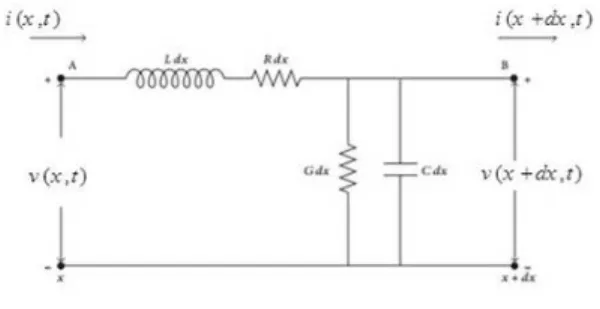
In this section, a detailed formalism for the telegraph formula in expressions of current for a segment of a broadcast line has been given. The circuit in Fig. 1 shows a tiny portion of the considered telegraph line.

Furthermore, the line is assumed to be partially non- conducting. In this case there is a leakage in the current and capacitance to earth. Let x be the separation from transferring ends

of the wire; on the wire, the current ( , )i x t is

considered for a specific position at any time; on the cable, the voltage ( , )v x t is considered at

a specific position at any time.

Fig 1: Design of the leaking telegraphic transmission line.

The voltage across both the resistor (R), the inductor (L), and the capacitor (C) respectively read:

iR

v= . (1)

dt di L

v= . (2)



= idt C

v 1 . (3)

From Fig. 1 above we havev_B =v_A−(v_R +v_L). So, combining Eqs. (1-3) together one can write:

t i Ldx i Rdx t

x v t dx x v

∂ ∂ − − −

+ , ) ( , )= [ ] [ ]

( . (4)

Now taking dx→0 and talk the partial derivative of Eq. (4) with respect to x then, we have

t i L Ri x

t x v

∂ ∂ − − ∂

∂ ( , )₌

. (5)

In a similar way, the current iB can be written

as:

dx i v Gdx t

x i t dx x

i( + , )= ( , )−[ ] − _C . (6)

where

t v C i_C

∂ ∂

= .

Again differentiating Eq. (4) with relevant to t and iC with relevant to x one got the following telegraph equation:

i nm t i m n t

i x

i

c = ₂ ( ) ( )

2

2 2

2 ₊

∂ ∂ + + ∂ ∂ ∂

∂ _{. (7)}

where

L R m C G

n= , = and

LC c2 = 1 .

There is an easy solution in the case where the resistance per unit length of the wire, and the conductance of the insulation separating the outgoing and returning wires, are small. So let's say R is little in comparison with L/ , and C

G is little in comparison with C/ . One has L

to note that L/ has the same dimensions as C

resistance, and is known as the characteristic impedance of the line. If we put R and G equal to zero in Eq. (7), so that we have an ideal lossless cable, and the transmission of the potential is governed by its inductance and capacitance per unit length alone, the equation becomes simply

2 2

2 2

2 ₌

t i x

i c

∂ ∂ ∂

∂ _{. (8)}

3. ANALYTIC SOLUTION OF THE

In order to obtain a solution for the Eq. (8), we consider the following initial conditions

) ( = ,0) ( ), ( = ,0)

( x x

t i x

x

i α β

∂

∂ _{. (9)}

and the boundary conditions ) ( = ) (1, ); ( = )

(0,t f t i t g t

i . (10)

In our following computations, we will consider f(t)= g(t)=0. We will search for a solution for Eq. (8) having the separable form:

) ( ) ( = ) ,

(x t A x B t

i ⋅ . (11)

Therefore Eq. (8) reads: ) ( ) ( = ) ( ) ( 2 t B x A t B x A

c ′′ ′′ . (12)

That is equivalent with:

2

2 _{( )} =

) ( = ) ( ) ( p x A x A t B c t B − ′′ ′′

. (13)

Thus we have x− _{dependent differential} equation of second order:

0 = ) ( ) ( 2 x A p x

A′′ + . (14)

with the conditions: 0 = (1) = (0) A

A . (15)

According to the rules used in solving DE's [21- 23], the characteristic equation has the complex roots: λ_1,2 = ±pi and as a result, the solution

will be: ) ( sin ) ( cos = )

(x a1 px a2 px

A + . (16)

Using the considered initial conditions, we have:

0 = = (0) a₁

A . (17)

N ∈   k k p p p a A , = 0 = sin 0 = sin = (1) 2

π

. (18)

Therefore, we have the solution:

N

∈

k

x

k

x

A

_k

(

)

=

sin

(

π

),

. (19)

The second differential equation (t−_dependent) is:

0

=

)

(

)

(

2 2

t

B

p

c

t

B

′′

+

. (20) Again referring to the rules used in solving DE's

[21- 23], the characteristic equation has the complex roots:

λ

_1,2

=

±

cpi

=

±

ck

π

i

, and as a result the its solution takes the form:

N

∈

+

w

kc

t

k

t

kc

u

t

B

k k k

),

(

sin

)

(

cos

=

)

(

π

π

. (21)

Thus the solution of Eq. (8) is:

) ( sin ) ( sin ) ( cos = ) ,

( k x

t kc w t kc u t x i k k

k π π

π ⋅      

+ . (22)

and the form of the general solution will be:

) ( sin ) ( sin ) ( cos = ) , ( 1 = x k t kc w t kc u t x i k k k π π π ⋅       +



∞ . (23)

Finally, in order to obtaina_k, and b_k we use the

initial conditions defined in Eq. (9) and taking into account the Fourier series [24- 26] we have:

dx x k x u x x k u x i k k k ) ( sin ) ( 2 = ) ( = ) ( sin = ,0) ( 1 0 1 = π α α π





∞ 

. (24)

kpixdx x kc w x x n kc w x t i k k k sin ) ( 2 = ) ( = ) ( sin ) ( = .0) ( 1 0 1 = β π β π π





 ∂ ∂ ∞

. (25)

Now in order to obtain a solution for the Eq. (7), with the initial and boundary conditions (9), (10), we have the form:

2 2 2 2 = = p c nm B B c m n B c B A A − + ′ + + ′′ ′′

. (26)

with the solution: ) ( sin = )

(x k x

A_k π . (27)

and the second differential equation: 0 = ) ( ) ( 2 B p nm B m n

B′′+ + ′+ + . (28)

with the discriminant of characteristic equation:

2 2 2

2 _{4 =}

) (

= n−m − k −a

∆ π and the complex

roots 2 2 = 1,2 a i m n ± + −

   

 

     

+

     

+ −

t a w t a u

e t

B t _{k k}

m n

2 sin 2

cos =

)

( 2 _{. (29)}

Therefore

) ( sin

2 sin

2 cos =

) ,

( 2 _{k x}

t a w

t a u

e t x i

k k t m n

k ⋅ π

   

 

   

 

     

+

     

+ −

. (30)

and the general solution for telegrapher's equation (7) is:

) ( sin

2 sin

2 cos =

) , (

1 =

2 _{k x}

t a w

t a u

e t x i

k k

k t m n

π

⋅

   

 

   

 

     

+

     



∞

+ −

.(31)

with

dx x k x u

k =2 ( )sin( )

1

0

π

α



. (32)

dx x k x m n a

w_k ( )sin( ) )

( 8 =

1

0

π

β



+

− . (33)

4. NUMERICAL METHOD

This section approaches the evolution in time of the intensity of the current that passes through the transmission line of the telegrapher. For a better accuracy, we realized a parallel using the numerical analysis between equation (7) and equation (8). In our study, we have considered six cases that are encountered in the real life for the boundary conditions. The evolution of the current's intensity is considered for different

values of time:

0.8 = 0.6; = 0.4; = 0.2;

= t t t

t andt=1. With

star symbol is represented the variation of )

, (x t

i from equation (7) and with continuous

line is represented the variation of i(x,t) from equation (8).

Typical order-or-magnitude values for a telephone cable might be about

1 11

10 5

= × − Fm−

C and L=5×10−7Hm−1 , and,

giving a speed of about 2×108ms−1 _{or about}

3 2

of the speed of light in vacuum . If we require to solve the general case Eq. (7) we have to choose

R _{so that it is comparable in size to L/ , C}

and G so that it comparable in size to C/ . L

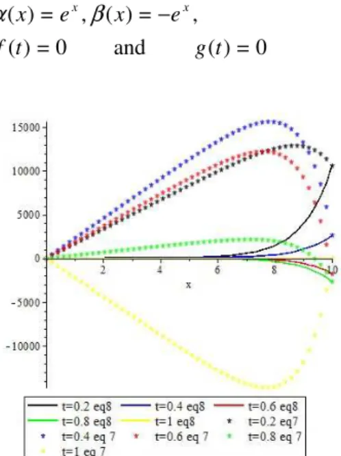
We can consider the following boundary conditions enumerated below in five cases. Case One:

0 = ) ( and 0 = )

( )=sin( ), ( )= sin( ), (

t g t

f

x x

x

x β −

α

Fig. 2: Comparison between (7) and (8) for the first considered case.

Case Two:

0 = ) ( and 0 = )

( )=sinh( ), ( )= cosh( ), (

t g t

f

x x

x

x β −

α

Fig. 3: Comparison between (7) and (8) for the second considered case.

0 = ) ( and

0 = ) (

, = ) ( , = ) (

t g t

f

e x e

x x β − x

α

Fig. 4: Comparison between (7) and (8) for he third considered case.

Case Four:

(1) sinh =

) ( and 0 = )) (

, ) sinh( 2 = ) ( , ) sinh( = ) (

2t

e t g t

f

x x

x x

−

− β

α

Fig. 5: Comparison between (7) and (8) for the fourth considered case.

5. RESULTS AND DISCUSSION

The evolution in time of the intensity of the current that passes through the transmission line of the telegrapher has been plotted against time for the five cases considered in Sec. 5, as shown in Figs. 2- 5, respectively. In first case, we can observe (Fig. 2) that the intensity of the current varies asymmetric for equation (7) and for the

equation (8), we can observe that the behavior of amplitude is symmetric. The intensity in case of equation (7) is dissipating. While for the second case, we observe (Fig. 3) that the signal given by the equation (8) is amplified and for the equation (7) the signal is dissipating.

For the third case, we observe (Fig. 4) that the signal as a similar behavior as the second case, but the values of current intensity is considerable bigger than in previous case. The current's intensity in the fourth case has a sharper growth for (8) in contrast to (7). After x=1 the ratio is changed as it is clear from Fig. 5.

Figure 2 shows that the current intensity behaves in nearly sinusoidal way for equation (8) while it is not behaving sinusoidal for equation (7). Figures 3, and 4 show that the current intensity for equation (7) is higher than that of equation (8) for the same time and there is no similarity between the behaviors of them. Finally, it is clear from Fig. 5 that the current intensity for equation (8) is always higher than that of equation (7) and the two behaviours are nearly similar to each other.

6. REFERENCES

[1] L. Hopf. Introduction to the Differential Equations of Physics. Dover; Notations, Name inked on Fep edition (1948).

[2] M.Tenenbaum. H. Pollard. Ordinary Differential Equations. Dover Publications, INC., New York. 1963.

[3] H. Bateman. Partial Differential Equations of Mathematical Physics. 1st edition. Cambridge University Press. 1932.

[4] David V. Kalbaugh. Differential Equations for Engineers: The Essentials. 1st Edition. 2017 [5] E. Kreyszig. Advance Engineering Mathematics. 9th

edition. Wiley eastern Pvt. Ltd. (India). 2006 [6] B. S. Grewal Higher Engineering Mathematics.

Khanna publication, New Delhi. 2014

[7] G. Bohme, Non-Newtonian fluid mechanics. New York: North-Holland; 1987.

[8] R.K. Mohanty, M.K. Jain, An unconditionally stable alternating direction implicit scheme for the two space dimensional linear hyperbolic equation, Numer. Methods Partial Differ. Equ. 17 (6) (2001) 684–688.

Boundary Elem. 34 (1) (2010) 51–59.

[10] H. Pascal, Pressure wave propagation in a fluid flowing through a porous medium and problems related to interpretation of Stoneley’s wave attenuation in acoustical well logging. Int J Eng Sci 24 (1986):1553–70.

[11] O. Heaviside, Electromagnetic theory, Chelsea Publishing Company, New York, Vol-2 (1899). [12] J. Banasiak, J.R. Mika, Singular perturbed telegraph

equations with applications in the random walk theory, J. Appl. Math. Stoch. Anal. 11 (1998) 9-28. [13] V.H. Weston, S. He, Wave splitting of the telegraph

equation in and its application to inverse scattering, Inverse Problems, 9 (1993) 789-812. [14] P.M. Jordan, A. Puri, Digital signal propagation in

dispersive media, J. Appl. Phys. 85 (1999) 1273- 1283.

[15] Vineet K. Srivastava, Mukesh K. Awasthi, R. K. Chaurasia, and M. Tamsir. The Telegraph Equation and Its Solution by Reduced Differential Transform Method. Modelling and Simulation in Engineering. Volume 2013, Article ID 746351, 6 pages

[16] R. Abazari and M. Ganji, “Extended two-dimensional DTM and its application on nonlinear PDEs with proportional delay,” International Journal of Computer Mathematics, vol. 88, no. 8, pp. 1749–1762, 2011.

[17] R. Abazari and M. Abazari, “Numerical simulation of generalized Hirota-Satsuma coupled KdV equation by RDTM and comparison with DTM,” Communications in Nonlinear Science and

Numerical Simulation, vol. 17, no. 2, pp. 619–629, 2012.

[18] Y. Keskin and G. Oturanc, “Reduced differential transform method for solving linear and nonlinear wave equations,” Iranian Journal of Science and Technology A, vol. 34, no. 2, pp. 113–122, 2010. [19] Y. Keskin and G. Oturanc¸, “Reduced differential

transform method for partial differential equations,” International Journal of Nonlinear Sciences and Numerical Simulation, vol. 10, no. 6 pp. 741–749, 2009.

[20] G. NHAWU∗, P. MAFUTA, J. MUSHANYU. THE

ADOMIAN DECOMPOSITION METHOD FOR NUMERICAL SOLUTION OFFIRST-ORDER DIFFERENTIAL EQUATIONS. J. Math. Comput. Sci. 6 (2016), No. 3, 307-314

[21] M. Tenenbaum, and H. Pollard. Ordinary Differential Equations. Dover Publications; Revised ed. Edition. 1985

[22] Earl A. Coddington. An Introduction to Ordinary Differential Equations. Dover Publications; Unabridged edition (1989)

[23] H. S. Bear. Differential Equations: A Concise Course. Dover Publications; Revised ed. edition (1999) [24] Robert T. Seeley. An Introduction to Fourier series

and Integrals. Dover Publications. 2006

[25] Phil Dyke. An Introduction to Laplace Transforms and Fourier Series. 2nd edition. Springer. 2014 [26] Rupert Lasser. Introduction to Fourier Series. Marcel

Dekker, Inc. 1996

ABORDARE MATEMATICĂȘI NUMERICĂ PENTRU ECUAȚIA TELEGRAFULUI

Rezumat: În acest studiu, considerăm ecuația diferențială parțială de ordinul doi cunoscută numită ecuație telegrafică.

Această ecuație este scrisă în termeni de tensiune și curent pentru o secțiune a unui suport de transmisie și are multe

aplicații în mai multe câmpuri, cum ar fi propagarea undelor, teoria deplasării aleatorii și analiza semnalului. În această

lucrare, am derivat mai întâi ecuația telegrafului. Ca al doilea pas, am rezolvat problema valorii de limită a ecuației

telegrafului în mod analitic prin utilizarea seriei Fourier. În cele din urmă, este studiată și obținută soluția numerică

pentru ecuația telegrafistului pentru diferite cazuri de condiții inițiale și pe frontieră.

Hussein SHANAK, Professor PhD, Palestine Technical University- Kadoorie, College of Applied Sciences, Dep. of Physics, P. O. Box 7, Tulkarm, Palestine. [email protected].

Olivia FLOREA, Professor PhD, Faculty of Mathematics and Computer Science, Transilvania University of Brasov, Romania. [email protected].

Noorhan ALSHAIKH, Lecturer MSc, Palestine Technical University- Kadoorie, College of Applied Sciences, Dep. of Physics, P. O. Box 7, Tulkarm, Palestine. [email protected]. Jihad ASAD, Professor PhD, Palestine Technical University- Kadoorie, College of Applied