An analysis of influential methodological practices in consumption based accounting methods

(1)

AN ANALYSIS OF

INFLUENTIAL

METHODOLOGICAL

PRACTICES IN

CONSUMPTION-BASED

ACCOUNTING METHODS

(2)

1

Acknowledgements

The author would like to thank Professor Nick Hewitt for academic support and guidance through this research project and Lancaster University for the continued support

throughout. She would also like to thank Small World Consulting Ltd. for allowing access to their models and knowledge base throughout the research process, and particularly Mike Berners-Lee and Robin Frost for their commercial and academic advice.

Declaration

I, Cara Kennelly, declare this work to be entirely my own and not published or submitted anywhere else or for any other merit.

(3)

2

Figure 4. The average carbon emissions factor calculated by each of the different input-output models as a percentage of the process-based life cycle assessment with gap analysis. Model acronyms are: Process-based life cycle analysis [PBLCA], PBLCA supplemented with gap analysis [PBLCA + gap analysis], Carnegie Mellon University [CMU SRIO], Department for Farming and Rural Affairs [DEFRA MRIO], Multi-regional Small World Consulting Ltd. model [SWC MRIO] and Small World Consulting Ltd. single region model [SWC SRIO] ... 25

Figure 6 Comparison of carbon emissions factors for the manufacture of iron and steel ... 30

Table 1 Metadata of input-output models compares in this study ... 13

(6)

5

Abstract

A key tenet of the work to mitigate anthropogenic climate change is to reduce carbon emissions. An entity; be it individual, company, or nation state, is more able to reduce their carbon dioxide equivalent emissions if they can be monitored and attributed, and their effects measured. The current state of carbon accounting methods does not consistently meet the standards required to tackle this global challenge, therefore this study aimed to identify key methodological practices affecting carbon accounting models and to assess the use of the system boundary.

Models currently available are either input-output based, (using macro-economic analysis), process-based, (using specific carbon emissions attributes through a life-cycle), or a hybrid of the two. A detailed comparison was made and the findings applied to a case study assessing the carbon burden of copper wire. An industry-leading process-based model was analysed using gap analysis and system boundary selection, and identification methods assesed.

Key methodological factors were found to be the inclusion of multi-regional data and sensitivity to the economic situation embodied in the model. Multi-regional data was found to increase carbon accounting model accuracy by reducing the need to make methodological assumptions

(7)

6

1. Introductory material

1.1. Literature and background

Climate change is arguably the most important environmental issue faced by humanity (IPCC, 2014), and a key part of addressing climate change is reducing the emissions of greenhouse gases associated with specific goods and services; often called a ‘carbon footprint’. The goods and services businesses provide are key sources of carbon dioxide and other greenhouse gases (collectively known as carbon dioxide equivalents: CO2e). Estimating the magnitude of emissions allows mitigation efforts to be directed more strategically; particularly important following ratification of the Paris Climate Agreement (November 2016) and anticipated zero-carbon policies.

1.1.1. Historical carbon accounting methods

Estimation of carbon footprints has had a varied methodological history. Net energy analysis (NEA), which measures the use of resources for valuable work within the economy, was an important forerunner to life cycle analysis (LCA). The practice of carbon footprinting began as the life cycle analysis of products and their impacts across a range of environmental issues. Life cycle

analysis is a holistic tool for evaluating full ‘cradle to grave’ environmental impacts of a product

or service, from initial extraction of raw resources (cradle) to the final disposal (grave) (Ayres, 1995; Suh et al., 2004). This method became a key method of making rational judgements on the environmental loads of end-use products (Ayres, 1995) which itself is crucial to making products with environmental awareness. Life cycle analyses have inherent errors due to a number of issues including unreliable measurements, estimates and assumptions; bias in original source data; temporal, geographical and technological miscorrelation; and deficiencies in knowledge of the systems in question (Lenzen, 2000).

1.1.2. Input-output carbon accounting models

Input-output analysis is a ‘top-down’ technique making use of financial transaction data to

monitor and account for the complexities of modern economic systems (Lenzen, 2000). By

applying known environmental data to this method it can be “environmentally extended”, creating the ‘EEIO’ (environmentally extended input-output) model. Since the initial creation of the input-output economic model by Leontief in the 1930s, it has been successfully extended internationally with national and regional input-output tables being adopted as a United Nations standard (Wiedmann, 2009), however the UK was the first country to report regular

consumption-based accounts (Defra, 2014).

(8)

7 operation is simple, and the necessary data input minimal (Wiedmann, 2009). Input-output analysis is particularly useful for capturing upstream emissions which contribute significantly to scope 3 emissions (Wiedmann, 2009).

Recently input-output models, previously describing only a single region of production and trade, have been redesigned to represent multiple regions, thus better representing the globalised nature of modern commodity trade. However, this has substantially increased the data requirement of input-output models (Andrew et al., 2009). Single-region models focus on only the production and trade within the borders of the country in question, whereas multi-regional models take into account the imports of commodities from outside the national boundaries. This has presented methodological challenges, namely the sourcing and integration of trade data, both multi- and uni-directional, into consumption-based carbon accounting methods resulting in greater complexity, however benefits in accuracy outweigh the costs which are not untenable (Andrew et al., 2009) and thus the multi-regional input-output consumption-based accounting model has become the benchmark standard.

However, input-output analysis has inherent limitations and uncertainties:

Firstly, each input-output model sector is assigned an embodied value for outputs which is homogenous across the sector (Bullard et al., 1978), despite the heterogeneous nature of the products and processes within that sector, thus leading to aggregation error (Suh et al., 2004).

Secondly, inflation (as the monetary value changes without necessarily affecting the physical quantities and therefore the associated carbon emissions; Bullard et al., 1978) and the infrequency of expenditure on expensive long-life products, can result in incorrect results for periods of atypical spend (Suh et al., 2004).

Thirdly, the constantly evolving nature of technological and economic systems results in frequent change of input-output economic categories which results in the need for constant monitoring and adjustment (Bullard et al., 1978). For example, the supply and use tables published annually by the Office of National Statistics has comprised of 110, 106 and now 105 industrial sectors.

Fourthly, the underlying tables require periodic updating to reflect the most recent national or regional figures or methodological updates. Without this financial and time expenditure the models would quickly become out of date and obsolete.

(9)

8

1.1.3. Process-based life cycle assessments

Process-based analyses are a ‘bottom-up’ approach to carbon accounting that involves itemised research of the carbon burden of a products life-cycle. They are prone to truncation error as the diminishing contribution of infinite terms results in a point where it is too costly or labour intensive to extend the system boundary beyond that point. However, the energy cost of processes beyond the system boundary can be very substantial (up to 87% in one analysis; Crawford, 2008). Potentially excluded processes have often never been assessed and therefore cannot be guaranteed negligible before being excluded from analysis - which may have impacts on the reliability of future comparative analysis (Suh et al., 2004).

Process-based analysis is high cost, labour-intensive, inflexible, has subjective boundary definition (Joshi, 1999) and the methods largely ignore supply chain aspects of environmental load (Lenzen, 2000). Simple processes require simple process-based carbon accounting - however the more complex the process the more complex the carbon accounting requirement (Weber et al., 2009). Thus, the results of this method are dependent on the effort expended by the analyst so a comparison of methods is somewhat irrelevant and has been deemed outside the scope of this study.

The amount of carbon embodied in a product estimated by process-based analysis is consistently lower than that estimated by input-output analysis (Lenzen and Dey, 2000; Crawford, 2008). However, there are exceptions which may be caused by better quality and/or quantity of process data than is usually available (Crawford, 2008). Despite the different process-based analysis approaches, truncation error is always significant as it contributes to the significant

underestimation of final life-cycle inventory values (Suh et al., 2004).

There is a significant disparity between the results of process-based analysis and input-output analysis (Crawford, 2008) and thus significant debate on the method by which to determine the system boundary between the two. The ability to fully understand optimal practice with boundary selection is key to successful hybridisation, and thus creation of a both a specific and systemically-complete carbon accounting method.

The use of cut-off thresholds in process-based analysis, (a system boundary beyond which supply chains are deemed insignificant) is unreliable and creates extremely variable analysis (Weber et al., 2009). Though each supply chain cut-off may be insignificant the sum of all cut-offs could be influential (Suh et al., 2004) and thus cannot be rigorously assessed for accuracy. Understanding the system boundary selection process and isolating the boundary itself is therefore key in the hybridisation of carbon models. System boundary selection decisions based on ISO standards are not typically made using a scientific basis (Suh et al., 2004). One scientific method on which to base system boundary selection decisions is structural decomposition analysis which is relatively easy to implement, requiring only excel processing, thus lending itself to both organisational accessibility and scientific rigour.

1.1.4. Hybrid carbon accounting methods

(10)

9 carbon emissions which the process-based analysis then calculates accurately. The input-output model is then used to calculate the remainder of the carbon burden as defined by gap analyses (Minx et al., 2008; Bullard et al., 1978; Treloar, 1997; Suh et al., 2004). This ideal is used within this study as an assumed best practice as it is the most accurate method currently available to estimate actual carbon emissions, unmeasurable with current technology.

Within business carbon monitoring, scope one and two emissions (the direct emissions from point of sale and indirect emissions from energy and electricity use respectively) are often assumed to be more significant that scope three (other indirect emissions) (Wiedmann, 2009), however this is not always the case (Weber et al., 2009). In a hybrid approach to carbon footprinting, emission hotspots can be readily identified using the broader input-output approach. By then combining with the process-based approach, the intention is for to gain specificity in key areas, as well as complete economic coverage. A significant benefit of the hybrid model over others is the system-completeness that merging top-down and bottom-up

approaches brings (Wiedmann, 2009), as well as the increased cost-effectiveness and specifiable accuracy (Bullard et al., 1978). These improvements ledto the results of hybrid models having consistently larger carbon values than those of purely process or input-output models (Crawford, 2008) and thus hybrid approaches have been recommended by multiple scholars (Minx et al., 2008; Lenzen, 2002). At its core a hybrid carbon model is the use of both process- and input-output based databases and the application of a system boundary selection process to describe where to use each model in order to utilise the best of each methodology.

1.1.5. Consumption-based accounting and the UK

Consumption-based accounting has dominated carbon accounting methods more recently due to

it’s methodological grounding in economics. Where production-based accounting methods can show you only a limited part of the carbon emissions of a product, an input-output model can describe the entire supply chain, an increasingly important dimension of the environmental impact of products in an increasingly complex market and world. Analyses of supply chains through consumption-based accounting can help identify and address risks that are intrinsically tied to procurement, such as resource taxation, price volatility and availability shocks (Owen et al., 2017). It is crucial for a governing body, such as the UK but at any spatial or political scale, to have confidence in and an understanding of the causes, influencers and mitigation strategies for these risks. Accuracy and consistency in these analyses encourages stability in supply chains that can be made unstable by economic, political or environmental factors.

1.1.6. System boundary selection

This study aims to assess the effects of system boundaries in hybrid carbon accounting methods. Gap analysis will be undertaken to attempt to isolate aspects of the method or analysis to identify options to make future system boundary analysis more reliable and scalable.

(11)

10 system expansion (BSI, 2006). The physical allocation method uses data on the mass of

commodities used in the production of a given product or service and assigns carbon burden data to those figures to calculate the carbon footprint of the product. The economic allocation

method attaches environmental data to economic data and uses this matrix to assign the proportion of carbon burden of each input to a product to calculate the final carbon footprint. The system expansion method involves accounting for the displacement factor of co-products created during the production of the primary product.

System boundary identification using different methods cannot be compared to each other as they each use incomparable parameters and datasets in the selection process. It is therefore important not only to identify the most accurate system boundary selection method, but also the most widely adopted to ensure comparable carbon accounts across platforms. (For example, business reports and academic reports could be used in tandem if the methodologies were comparable and thus knowledge could be shared more easily and effectively). This is key to the future of carbon accounting as it will enable a more holistic approach to carbon emissions reductions.

Gap analysis is particularly important in isolating system boundaries within carbon accounting methods. By providing insight into the way input-output and process-based analyses work in conjunction, it allows a more accurate overall system boundary to be calculated. Whereas input-output analysis achieves completeness it can be prone to overestimation, conversely process-based analysis sacrifices completeness for specificity. Gap analysis allows valuable insight into the trade-offs of locating the system boundary in different places in relation to each method.

1.2. Aims and objectives

The intention of this study is to compare the calculated kgCO2e per pound sterling (£) of spend from different input-output models and subsequently analyse system boundary selection approaches and their impact within current hybrid carbon footprinting methods. Comparative techniques and statistics on both specific and general examples afford insight into recent carbon accounting practice and for this to be understood in terms of both individual techniques and broad use of carbon accounting methodologies. An improved understanding of carbon

accounting mechanisms will be key in the future reduction of carbon emissions particularly for end users. Despite recent recognition that carbon accounting methods must be constructed with the end user in mind (Owen et al., 2017), there is much progress to be made, and so this study aims to maintain the interests of specifically commercial end users.

1.2.1. Aims

• Compare the calculated emissions intensities of four input-output carbon accounting models.

• Identify influential methods in input-output carbon accounting models and their impact on calculated emissions intensities.

(12)

11

1.2.2. Objectives

• Use confounded and unconfounded (multiple variable and single variable) analysis to identify and assess the strength of influential methodological practices in input-output models.

• Conduct structural path and gap analysis on industry sectors with simple supply chains.

• Identify industry sectors for which the input-output models most agree and most disagree and compare each model within these sectors to assess significant methodologies.

(13)

12

2. Methodology

A detailed breakdown of the methodology used in each stage of this research will be explained and justified in this chapter.

Models were sourced directly from the creator. Where possible the models were publically available, however due to the lack of clarity in the methodology of publically available models and the requirement for meaningful analysis it was deemed appropriate to use a model for which the data was not directly publically available but whose methodology was completely

transparent, which was the case for the Small World Consulting Ltd. models, and thus a link to the 2011 model has been provided in table 1 for context. Small World Consulting Ltd. provided their two models with methodological papers and the Defra and Carnegie Mellon University models (and associated methodological papers) were downloaded from the associated webpages. These models and documents were analysed to isolate influential methodological practices using statistical measures such as range and mean. The prevailing model was then compared to the Argonne Laboratory GREET.net model in order to assess system boundary methodology using a case study on the carbon burden of copper wire. All methods were

undertaken using 2012 data and models were run both according to the published version of the model and in deconstructed ways, (as far as the methodological transparency would allow), in order to isolate the most influential methodological practices.

2.1. Input-Output Model Comparisons

2.1.1. Input-output Model Mechanics

The model mechanics on which input-output carbon emissions models are based is matrix algebra of national supply and use tables. As the name suggests, databases describing the supply (or input) and demand (or output) of a system are used to map the relationships between different elements of that system. In the case of carbon accounting the system is usually an economy, regional, national or international, and the different elements are industries within that economy. The relationships are mathematically described using the leotief inverse which follows the equation:

𝐿 = (𝐼 − 𝐴)−1

Where I represents the identity matrix and A represents the technical coefficient matrix. A detailed description of the theory behind this equation and the steps required to build an input-output model can be found in (Miller and Blair, 2009).

2.1.2. Model Descriptions

There are a number of different carbon accounting models available in the UK and

(14)

[image:14.595.109.526.89.436.2]

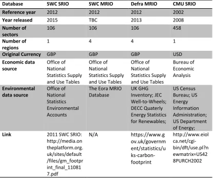
13 Table 1 Metadata of input-output models compares in this study

Database SWC SRIO SWC MRIO Defra MRIO CMU SRIO Reference year 2012 2012 2012 2002

Year released 2015 TBC 2013 2008

Number of sectors

106 106 106 458

Number of regions

1 4 4 1

Original Currency GBP GBP GBP USD

Economic data source

Office of National Statistics Supply and Use Tables

Bureau of Economic Analysis Environmental data source Office of National Statistics Environmental Accounts

The Eora MRIO Database UK GHG Inventory; JEC Well-to-Wheels; DECC Quaterly Energy Statistics for Renewables; US Census Bureau; US Energy Information Administration; US Department of Energy;

Link 2011 SWC SRIO: http://media.on theplatform.org. uk/sites/default /files/gm_footpr int_final_11081 7.pdf

N/A https://www.g

ov.uk/governm ent/statistics/u ks-carbon-footprint http://www.eiol ca.net/cgi-bin/dft/use.pl?n ewmatrix=US42 8PURCH2002

2.1.2.1. Carnegie Mellon University Environmental

Input-Output Life Cycle Assessment

The Carnegie Mellon University Environmental Input-Output Life Cycle Assessment model was developed by the Green Design Institute of Carnegie Mellon University. It uses 458 industrial sectors categorised using the North American Industry Classification System (NAICS). Gross fixed capital formation (GFCF) and high-altitude factors for aircraft emissions of greenhouse gases are not included in the model. Gross fixed capital formation is a measure of the fixed assets used continuously for over a year, such as buildings (Eurostat, 2013) and represents the long-term carbon burden of these fixed assets. This is a single-region model based on the United States that uses old, incomplete data with inherent uncertainty, thus any findings based on this analysis should be treated with caution. Use and end-of-life phases of the product life-cycle, (otherwise known as scope 3 emissions), are not included in the Carnegie Mellon University model. This is therefore not a full life cycle assessment despite the title of the model.

(15)

14 sectors to the corresponding sector in the UK models. These calculations can be found in

appendix A.

2.1.2.2. Department for Environment, Food and Rural

Affairs (Defra)

Defra is a UK government department that uses data from the Digest of UK Energy Statistics (DUKES). This is a multi-regional model that distinguishes four world regions: the UK, countries within both Europe and the OECD, non-European OECD countries, and non-OECD countries (Minx et al., 2008). This data source and model is updated annually and uses the Standard Industrial Classification (SIC) categorisation for its industrial sectors. There is inclusion of gross fixed capital formation, however no high-altitude factor is included in the Defra calculations and they do not account for scope 3 emissions consistently or precisely across sectors. There is a multiplier used to account for the non-CO2 effects of air travel, such as the radiative forcing; however this is not as influential as a direct high-altitude factor would be. As a multi-regional model this model, and the Small World Consulting Ltd. multi-region input-output model described below, would require a much larger dataset thus making it more difficult to set up and update, however the trade data would more accurately represent the globalised supply chains (Andrew et al., 2009).

2.1.2.3. Small World Consulting Ltd. Single-Region

Input-Output Model

Emissions estimates are calculated predominantly based on supply and use tables from the Office of National Statistics (ONS) using conversion factors from Defra on data relating to travel, fuel and energy consumption and national purchases of products and services from the Office of National Statistics, with additional calculations based on Small World Consulting Ltds’ specific

methodology. Unlike all other models, this includes both gross fixed capital formation and a high-altitude factor for aircraft emissions. In this model all supply chain pathways from the air

transport sector are multiplied by 1.9 to reflect the increased impact of releasing greenhouse gases at altitude compared to releasing them at ground level. This factor of 1.9 is used in

accordance with a Defra reporting guidelines publication where the 1.9 high altitude factor figure was published in footnotes.

2.1.2.4. Small World Consulting Ltd. Multi-Regional Model

(16)

15

2.1.2.5. Process-Based Life Cycle Assessments

The process-based life cycle assessments used to compare the input-output models in chapter three are based on the Defra process-based life cycle analysis figures published relating to 2012. Data was extracted from Defra and the Office of National Statistics relevant databases and other individually researched datasets. Simple calculations were undertaken to establish the kilograms of carbon dioxide equivalent greenhouse gases emitted for every £1 of spend in each of the industries. Each industry was disaggregated into relevant product types to reflect the specificity ideally gained through process-based life cycle analysis techniques over input-output methods and thus to create a more accurate and objective comparative database. For example, the electricity production, transmission and distribution industry was broken down into the following product groups: UK Domestic, UK Industry, UK Industry & Domestic, UK Total, UK Average. The same breakdown was conducted on US-produced electricity to reduce the impact of the different geographical sources of models on the comparison of the models and methods.

2.1.2.6. Important Notes

The theoretical basis of the Carnegie Mellon University model is the economy of the United States. Therefore it is not directly comparable to the other models as the theory of the Defra and Small World Consulting Ltd. models is based on UK economics and industry. All carbon factors, as produced by the relevant models, represent the kilograms of carbon incurred during the

production of £1 worth of goods in that sector. As such, all models are comparable at the final results stage as presented in this study.

2.1.3. Consumer Price Index Correction

Due to the limited availability of input-output carbon accounting models with sufficient published methodology to conduct this analysis and a requirement for methodological diversity it was decided an inflation-based correction of some older models would be better suited than a smaller sample size. The consumer price index (CPI) was used to correct data relating to time points before 2012 using inflation so that they better aligned with the economic data described in the carbon accounting models that represented the year 2012. In this analysis, the Carnegie Mellon University model was the only model that consumer price index correction was applied to.

(17)

16 For the calculation of the correction ratio the industry-specific consumer price index for the base year, in this case 2002, was divided by the target year, which would be 2012 for the Carnegie Mellon University model. This method follows basic mathematical principles of ratios. The resulting ratio from that calculation was then multiplied by the conversion factors produced by the Carnegie Mellon University input-output model to calculate the conversion factors corrected to the 2012 economic value.

2.1.4. Accuracy Analysis

Within the accuracy analysis a process-based life cycle assessment was used as a benchmark which all input-output models were compared to. This benchmark represented a theoretical 100% of life cycle carbon emissions comprising a hybrid life cycle assessment (process-based, input-output, and gap analysis assessments) for the mining of coal and lignite, the manufacture of coke and refined petroleum products and the electricity production, transmission and distribution industry sectors against which the input-output models in question and the process-based assessment without the gap analysis were compared. This enabled the calculations to

identify methodological practices that were more likely to lead to the assumed ‘correct’ carbon

emissions factor.

These industries were chosen as they were considered simple enough that a process-based analysis method would represent them relatively accurately and their databases contained enough supply chain documentation that any findings would be relatively easy to contextualise. These parameters meant that detailed and in-depth analysis was possible enabling a better understanding of any results.

While this method was not ideal due to the significant issues with the process-based

methodology, as discussed in the introductory material, it was deemed the best option available to this study. A benchmark had to be used that was not based in input-output methodology in order to ensure the any findings from input-output model comparisons were independent. As there is no way to directly measure the full life cycle carbon burden of a product, industry, service, etc. process-based analysis was used. A process-based analysis was conducted of the three industry sectors in question and a gap analysis applied to each of these industries individually. This gap analysis resulted in a ratio of truncation error which was applied to the process-based analysis result to increase it to a value that was both specific and systemically complete. This hybrid carbon accounting method used established process-based databases, namely Defra and Office of National Statistics, and gap analysis ratio application which, for the purposes of this study, was considered best practice. It is acknowledged that there are issues with this methodology and that in the real world it would not represent a best-practice case as it is is still subject to many of the methodological issues associated with process-based carbon accounting methods.

2.1.5. Precision Analysis

The degree of precision an input-output model achieved was based on the degree of agreement between multiple input-output models. Each of the original models was manipulated to

(18)

17 using purchasers prices to find the final conversion factors, and then run again using producers prices, creating two versions of the same model but with variable methodology. Each of these variants was collated and used to calculate mean values for each industry sector. In total there were 30 variations of the models, sixteen representing the Small World Consulting Ltd. single-region model, ten from the Small World Consulting Ltd. multi-single-region model , two from Carnegie Mellon University and two from Defra. The potential for the greater amount of Small World Consulting Ltd. models compared to either Carnegie Mellon University or Defra is a result of the lack of transparency of the methodological papers provided by the latter two organisations. The implications of this are discussed in more detail in chapter 6.1.

In this instance for Small World Consulting Ltd. single-region input-output model, although the final results and in-depth methodology was available online the model itself was not publically available. Access to the model for academic purposes was requested and provided readily, and the full model was manipulated using information from the publically available methodology papers. This method of accessing the model allowed a greater level of manipulation and

therefore the Small World Consulting Ltd. single region model contained the greatest number of variations in this comparative analysis.

2.2. Copper Wire Case Study

Analysis of the system boundary was undertaken on the case study of 1 kg of copper wire production. Consumption-based accounting analysis was conducted, supplemented with gap analysis and supported by related research. The aim of this was not only to identify and isolate the system boundary within hybrid carbon emissions models but also to attempt to identify the potential to make any part of this process more generic in order to make it more accessible to a wider audience.

2.2.1. Argonne GREET.net model methodology

As the GREET.net model is currently being dismantled by the Argonne National Laboratory the detailed methodology papers do not exist (Dieffenthaler, 2016). An in-depth understanding of the processes is therefore not possible, however the copper wire supply chains data were supplied by personal correspondence from the Argonne National Laboratory and the following system boundary analysis was based on that data.

The Argonne GREET.net model is based on the US economy, but the input-output model it is hybridised with is based in the UK. For the purposes of this study this is not critical as the intent is to study the method rather than the results. However it does mean that this exact method should not be undertaken outside of this study. In all real-world cases the input-output and process-based methods intended for hybridising should represent the same individual or set of regional economy(ies) to ensure the highest levels of accuracy and reliability in the results.

(19)

18 the GREET.net model and thus caution should be taken when applying their process-based figures to other hybrid carbon model analyses.

For the commodity copper wire, the results of GREET.net describe specifically the drawing of the copper wire as it uses the following: virgin copper, petroleum as manufactured from crude oil by industrial boiler, coal (average US mix) as manufactured by industrial boilers, and electricity (average US mix). Embodied within the model methodology is the energy requirement at Chilean and American manufacturing locations, though at a significantly aggregated level.

2.2.2. Process-Based Life Cycle Analysis Methodology

The greenhouse gas process-based life cycle analysis used is the system boundary analysed for this study was from the Argonne GREET.net model. The GREET.net results for copper wire produced in 2012 were used to make the process-based model as compatible as possible with the input-output models by aligning the data temporally. The Argonne National Laboratory is based in the US but is a global research institution that produces thorough science in the form of reports, databases and models. As such it is a source of some of the best process-based analyses available in terms of breadth of products covered and detail included per product analysed.

Though there have been many academic publications of process-based life cycle analyses these have often been either so specific as to be irrelevant to most carbon intensity analyses (for example: Pearce et al., 2013; Hu, 2012; Stylos and Koroneos, 2014) and/or funded by businesses and hence may be biased (for example: Kumar et al., (2014) funded by HP and Ayushmaan Technologies; Zhang et al., (2015) funded by the Kunming Engineering Corporation Ltd). Even the methods used in life cycle assessments can be subject to biases, such as Steinmann et al. (2014) funded by ExxonMobil, who have a direct and vested interest in the results of carbon analyses yet proposes to refine and adjust the results of carbon footprints. A standardised approach, as this study works towards creating, is critical to enabling the widespread use and understanding of carbon footprints and life cycle analyses.

2.2.3. Gap Analysis

A gap analysis was undertaken by comparison of the input-output sectors of the Small World Consulting Ltd. single-region model to those included in the Argonne GREET model database and methodology papers. Where input-output sectors were not wholly included or excluded in the process-based analysis an effort was made to understand the extent to which the data that were included in the Argonne GREET.net analysis covered the full sector data of the input-output analysis. This ratio was then substituted into the gap analysis to calculate the amount of the input-output analysis covered by the process-based calculations.

(20)

(21)

20

3. Model Comparison Results

This chapter describes the findings of the input-output model comparisons undertaken between the Defra, Carnegie Mellon University, and Small World Consulting Ltd. single- and multi-regional input-output models. Two main methods of analysis are used to assess the ability of the models to replicate real world emissions, as estimated by their closeness to a process-based life cycle analysis conducted within this study (i.e. their accuracy, as defined below) and the ability of models to agree amongst themselves (i.e. their precision, as defined below). In-depth

comparisons are derived from the methodology documents provided by each organisation and, where possible, a structural path analysis of the results, the full workings and results of which are available in appendix A. The following documents are used in this methodological comparison:

• 2012 Guidelines to Defra/DECC’s GHG Conversion Factors for Company Reporting:

Methodology Paper for Emissions Factors

• Well-to-wheels Analysis of Future Automotive Fuels and Powertrains in the European Context, WTT Appendix 1: Description of individual processes and detailed input data (Edwards et al., 2011)

• About The EIO-LCA Method, available at: http://www.eiolca.net/Method/index.html, Green Design Institute, Carnegie Mellon University

• The 2002 US benchmark version of the economic input-output life cycle assessment (eio-lca) model, by C. Weber, D et al., Green Design Institute, Carnegie Mellon University, June 16, 2009

3.1. Accuracy Analysis

Accuracy in the context of this study refers to the proximity of an emissions intensity output to the actual emissions intensity of a given product. Input-output models have been criticised as being too generic in their analysis, as whole industry sectors are used to represent, in some cases, just one product. When a product is atypical of the industry sector it is produced in, this results in low accuracy of the input-output models result. Process-based analysis methods have the highest potential accuracy because they are bespoke and specific, and if enough time and money is invested in the analysis the truncation error can be reduced significantly enough to make it comparable to input-output results in terms of system completeness. Thus, detailed process-based analyses were undertaken of three extractive industries, with the simplest supply chains and the most reliable data sources, and these figures were compared to the results from the input-output databases by finding the percentage of the input-output figure that the process-based values covered. To analyse the impacts of different variables, the mean of all models with a specific variable was compared to the opposite methodological mean to obtain the extent of the influence of each variable.

(22)

21 methodological practice to be studied in the appropriate context. Unconfounded analysis

describes data with only one variable, and thus describes the impact of only one methodological choice on the industry sector carbon accounting results in isolation from other methodological choices. This analysis provides more clarity of the impact of each methodological choice and therefore its potential methodological importance for the accuracy of results. However, the isolation of the impact of each variable means that the influence of other methodological choices on the variable studied is not considered. As such, the inclusion of both confounded and

unconfounded analysis was deemed valuable.

A particularly important variable, not included in all models, is a correction factor for greenhouse gases emitted at high altitude by aircraft. This correction factor is designed to reflect the

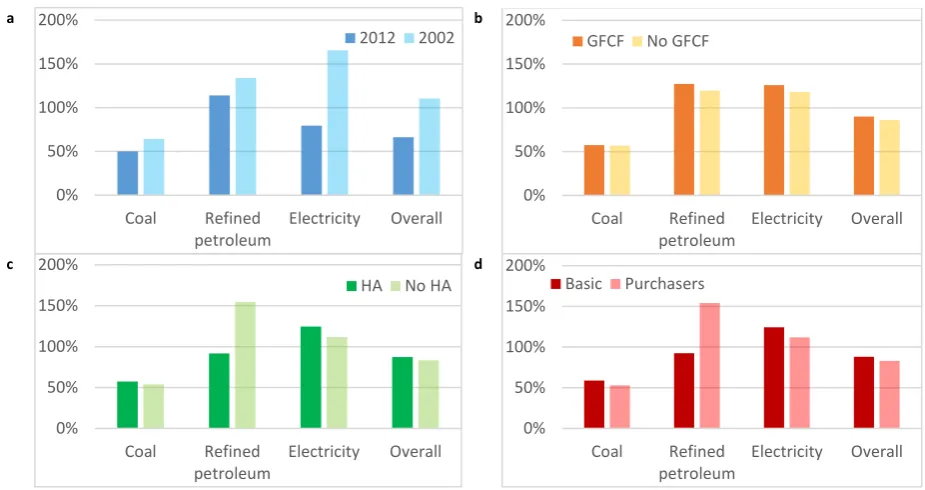
increased potency of greenhouse gases in the upper atmosphere, and the use of this factor increases the calculated carbon footprint of models that include it compared to those that do not. Within calculations it is applied to all air transport involved in the supply chains of a product or service, thus methodologically applied to the entire economic model, however, the total impact of the high-altitude factor is dependent on the reliance of that products supply chain on air transport. For example, the high-altitude factor is applied to both the manufacture of coke and refined petroleum products and the mining of coal and lignite. In the confounded analysis (figure 2) there was found to be a greater impact of the high-altitude factor on the manufacture of coke and refined petroleum products than on the mining of coal and lignite.

3.1.1. Confounded Analysis

(23)

22

a b

[image:23.595.94.557.67.312.2]

c d

Figure 1. Comparative graphs of the input-output analysis results of all models as a percentage of the process-based calculation with respect to a) year b) inclusion of gross fixed capital formation (GFCF) c) inclusion of a

high-altitude factor (HA) d) basic or purchasers’ prices

3.1.2. Unconfounded analysis

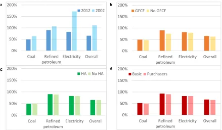
When the variables presented are not confounded (as in figure 2), based on the manipulation of the Small World Consulting Ltd. single-region model alone (as this was the model with the most accessible methodology), the apparent influence of each factor can be significantly reduced. For example, comparing figure 1c with 2c shows the almost non-existent impact of including or excluding a high-altitude factor on any of the sectors studied here. Figure 2c shows a maximum difference between high-altitude factor inclusive and exclusive models of 1.4%. This confounded and unconfounded results comparison suggests another methodological variable may have a stronger impact on the resulting estimation of the carbon footprint of the coke and refined petroleum products industry.

Other factors also had some impact, varying between methodology and industry sector. The inclusion of gross fixed capital formation is only a directly significant consideration in the case of the manufacture of coke and refined petroleum products (figure 2b), possibly due to the gross fixed capital formation embodied in refineries and the increased carbon burden they place on the commodity production compared to other industries.

There is minimal difference between the confounded and unconfounded analysis of the different years of data. This is likely due to the adjustments for inflation which are standardised and therefore lead to low variation between results. It is apparent that the 2002 values were larger than the 2012 values as the consumer price index adjustment would have increased the carbon emissions attributed to each pound sterling of spend in relation to economic adjustments, rather than assigning larger emissions intensities to the 2002 model than the 2012 models.

0% 50% 100% 150% 200% Coal Refined petroleum Electricity Overall

GFCF No GFCF

HA No HA

(24)

23

a b

[image:24.595.113.553.67.324.2]

c d

Figure 2. Unconfounded comparative graphs of the input-output analysis results of all models as a percentage of the process-based calculation with respect to a) year b) inclusion of gross fixed capital formation c) inclusion

of a high altitude factor d) basic or purchasers’ prices.

3.1.2.1. Confounded and unconfounded analysis conclusion

Both confounded and unconfounded variable analyses are useful in this study. The confounding variables analysis has been included as it highlights the relative importance of certain

methodological factors over others and allows a comparison of the non-independent variables in which their interdependencies can be analysed. This issue does not seem to influence either the electricity production or the mining of coal and lignite sectors. Their comparative figures,

discounting multi-regional models, are only ever a few percentage points different to calculations that include multi-regional figures, compared to up to 30 percentage points difference in the coke and refined petroleum products industry. This suggests a difference in production methods that implies that coke and refined petroleum products manufacture is more heavily dependent on international trade than either of the other comparative sectors.

This analysis also highlights the relative importance of different methodological practices within different industry sectors and the potential impact these practices, and their inclusion or exclusion within carbon intensity calculations, can have on final carbon emissions factor results. For example, consider the minimal impact of high-altitude generally, and the strength of the gross fixed capital formation influence in the refined petroleum industry. Such subtleties are likely be part of comprehensive understanding of carbon accounting in all industries.

3.1.3. Multi-regional data comparison

The influence of including multi-regional data in environmentally extended input-output models is potentially high but would not have been reliably compared in the previous analysis due to the

0% 50% 100% 150% 200% Coal Refined petroleum Electricity Overall 2012 2002 0% 50% 100% 150% 200% Coal Refined petroleum Electricity Overall

GFCF No GFCF

HA No HA

(25)

[image:25.595.135.498.231.445.2]

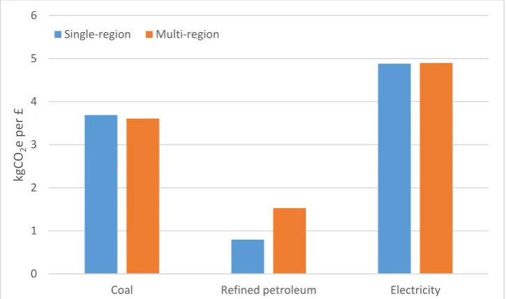
24 significant changes in methods required when including multi-regional data and the limited sample sizes as available in this study. As such, the Small World Consulting Ltd. single- and multi-region models have been compared directly for the industries of coal mining, refined petroleum products and electricity production, transmission and distribution. Theoretically, the inclusion of multi-regional data into an economic model representing the globalised markets of modern economies should increase the accuracy of results. This analysis found that changing the regions included by an input-output model had a limited impact on the carbon burdens calculated for coal mining and electricity industries, but increased the refined petroleum products industry.

Figure 3 Comparison of a single and multi-regional model produced by Small World Consulting Ltd. Model

Measureable impact of multi-regional data inclusion in these industries seems limited to refined petroleum products, with the methodological practice creating only a marginal difference in both the coal mining and electricity industries. This is likely due to the lack of imports in the electricity industry and the predominant source of coal imports to that of the UK coming from Europe, which has a similar carbon profile for coal to the UK. The refined petroleum products industry is more global in its trade, which could explain the difference.

The influence of the number of regions included in the model calculations has been hinted at but not fully examined. When all other variables are equal, there is no significant effect from using a multi-regional model apart from in the case of the manufacture of coke and refined petroleum products (figure 3). Within that industry sector there is a clear distinction between the single-region model, which calculates the smallest carbon intensity, followed by the multi-single-regional model and subsequently the process-based analysis.

0 1 2 3 4 5 6

Coal Refined petroleum Electricity

kgCO

2

e

p

er

£

(26)

25

3.1.4. Gap analysis

Although process-based methods have the potential for high accuracy in some sectors, they are always subject to some amount of truncation error and thus the inclusion of gap analysis gives the greatest likelihood of systemically complete accuracy. The theoretical ‘best practice’ has here

been assumed a hybrid of a detailed process-based life cycle analysis (PBLCA) with a gap analysis conducted on it from a robust input-output model. The resulting truncation error calculated as a percentage was then used to factor up the process-based life cycle analysis (PBLCA + gap analysis) to give a best estimate of actual emissions, as these are currently impossible to know.

[image:26.595.113.521.208.448.2]

Figure 4. The average carbon emissions factor calculated by each of the different input-output models as a percentage of the process-based life cycle assessment with gap analysis. Model acronyms are: Process-based

life cycle analysis [PBLCA], PBLCA supplemented with gap analysis [PBLCA + gap analysis], Carnegie Mellon University [CMU SRIO], Department for Farming and Rural Affairs [DEFRA MRIO], Multi-regional Small World

Consulting Ltd. model [SWC MRIO] and Small World Consulting Ltd. single region model [SWC SRIO]

Small World Consulting Ltd. produced the model with the greatest consistency of accuracy and the greatest accuracy with respect to this research (49% to 90%, figure 4). The Carnegie Mellon University model had the widest range of results (53% to 246%, figure 4) suggesting a low degree of accuracy across the full scope of the model. Production of coke and refined petroleum

products was found to be the industry sector with the greatest variability across models in this process-based analysis, with calculations covering 62% to 246% of the process-based analysis figure (figure 4). While a manufacturing industry, it is not as simple as the mining of coal and lignite extractive industry sector or as well-regulated and monitored as the electricity industry, possibly causing the differences between model estimations of this industry.

There is significant variation in the accuracy of each model according to comparison to the assumed best practice model, both between and within models. Of particular note in figure 4 is the Carnegie Mellon University estimation of refined petroleum products as 246% of the process-based life cycle assessment and gap analysis, which is likely due to the significantly lower prices of petroleum in the United States. However, not all disagreements in the data can be explained

0% 50% 100% 150% 200% 250% 300%

SWC SRIO SWC MRIO DEFRA MRIO CMU SRIO PBLCA + gap analysis

PBLCA

Electricity

(27)

26 so readily. The implications of truncation error and the related accuracy consequences are explored in further detail below.

3.1.4.1. The mining of coal and lignite

Although the gap analysis shows that for the mining of coal and lignite sector, the process-based analysis excluded 31% of the supply chain from its calculations, the final value is greater than that of the input-output models because the methodology for the process-based analysis included coal sourced globally. The process-based analysis of this industry sector produced a figure around 17% greater than the nearest of the input-output model results (figure 4). This was unexpected due to the different effects of truncation error of input-output and process-based

methodologies. UK input-output models broadly agree here at 48-52% of the process-based model, once adjusted for gap analysis results. One of the reasons that the process-based figure was so much larger than the input-output figure was the difference in the source of the coal used in each analysis. Input-output models used coal supplied from the countries they describe, i.e. UK or US coal depending on the model in this particular study, whereas the process-based figure was global. In the process-based model only 52% of the coal is assumed European, and only 18% from the UK (Edwards et al., 2011). The rest is from South Africa (16%), Australia (12%), the US (10%), Columbia (7%) and the Commonwealth of Independent States (3%). The similarities of these percentages is likely not a coincidence as the increased travel distance of this coal will have incurred a significant carbon burden due to the weight of coal and the implications of that weight on the carbon burden of transporting it. In addition, the difference in mining methods and quality of the coal mined likely impacted the carbon emissions calculated. For example, Australian open-cast mining leads to the release of methane as the coal is extracted. This methane emission

caused over 3% of Australia’s total carbon emissions in 2008 (Day et al., 2010). Thus, the impacts

of including global coal are substantial, in this case potentially increasing the carbon intensity by 48-82% based on calculations of propagations of the discrepancy from the extraction of coal to inclusion in the carbon models.

Despite the described issues with the interpretation of this sector some conclusions can be drawn with reasonable reliability. Defra calculated the value closest to the ‘best practice’, thus performed the best in this comparison in terms of model accuracy. While the other UK models performed similarly, the Carnegie Mellon University model calculated only 23% of ‘best practice’.

This was most likely due to the fact that it represented an entirely different supply chain.

3.1.4.2. The manufacture of coke and refined petroleum

products

(28)

27 was also the only input-output model to underestimate the carbon footprint of this industry, though by the comparatively small margin of 10%. The Carnegie Mellon University model

calculated a value of 246% of the ‘best practice’ model and thus performd the worst of all models

and all sectors compared. Unlike the other two sectors subjected to accuracy analysis in this study, for the manufacture of coke and refined petroleum products the Defra model

overestimated compared to the process-based value. It is unclear precisely why this is the case; however, it may be due to the fact that the petroleum coke figure used in the process-based analysis was based on a calculated liquefied petroleum gas carbon intensity that was scaled using a direct emissions ratio and thuse the input-output models are describing different products to the process-based analysis, leading to uncertainty.

3.1.4.3. Electricity production, transmission and distribution

The process-based analysis of electricity production, transmission and distribution was

represented with reasonable accuracy, in methodological terms. The Small World Consulting Ltd. single and multi-regional models were equally accurate when calculating electricity sector carbon intensities. No input-output model covered the full value calculated by the process-based analysis. Fluctuations in price are significant in the electricity industry and this may be a reason for the difference in carbon emissions intensities calculated by input-output and process-based models. However, the input-output models did marginally out-perform the process-based analysis when the gap analysis was excluded from the final process-based figure, supporting the knowledge that input-output models will calculate larger values for carbon intensities than process-based analyses alone. The Carnegie Mellon University model significantly under-estimated the process-based life cycle analysis figure, both with and without gap analysis, thus was the least accurate model for the electricity production, transmission and distribution sector.

3.1.5. Accuracy Analysis Conclusion

As accuracy here represents the closeness of the input-output model results to the process-based results with the addition of gap analysis, the accuracy of each model was assessed by identifying and calculating the input-output model results as a percentage of the process-based plus gap analysis results, the latter of which it has been established is the most likely to be closer to the true carbon burden of the industry. As such, the closer to 100% an input-output models results were, the more accurate that model was deemed to be. The Small World Consulting Ltd. single region model was found to be the most accurate, and most consistently accurate, input-output model over the three industry sectors analysed. Carnegie Mellon University’s model appeared

(29)

28 with some inconsistency of results, though much less pronounced than either the Carnegie Mellon University or Defra input-output models. Thus, both Small World Consulting Ltd. models showed the greatest accuracy of carbon intensity calculations.

3.2. Precision Analysis

In this context, ‘precision’ refers to the likelihood that multiple carbon emissions models will calculate the same emissions factor for a given industry sector, i.e. the closeness of each model to the mean of all models for any given industry sector. This type of precision was assessed by analysis of the difference between the mean of all available model variations for each respective industry sector to the individual model results for that industry in both real terms (kgCO2e/£ difference) and percentage differences. Precision can vary between both models and industry sectors and therefore each industry sector was analysed for precision independently of other industries. Comparison of each sector output from individual models to a calculated mean of all model outputs allowed for a comparison of the precision of calculations for each sector. Where models broadly agreed, such as sector 81, “Services to Building and Landscape”, these can be

said to have high statistical precision. Where models disagreed, such as sector 92, “Gambling and

Betting Services”, model precision was low. By comparing methodologies and influential factors of both high and low precision sectors the important methodological factors were isolated that will enable increased precision in future models. However, it should be noted that a high degree of precision does not necessarily imply a high degree of accuracy in model results.

Input-output sectors can be broadly categorised into four groups of similar industry types: extractive, manufacturing, distribution, services. Each of the industry sectors in these four broad categories have not only similar products but also similar supply chain structures, which

(30)

29

3.2.1. Low Agreement Industry Sector Examples

3.2.1.1. 19: Coke and refined petroleum products

[image:30.595.133.502.70.326.2]

Figure 5 Comparison of carbon emissions factors for the manufacture of coke and refined petroleum products

(31)

30

[image:31.595.132.501.68.304.2]

3.2.1.2. 24.1-3: Manufacture of iron and steel

Figure 65 Comparison of carbon emissions factors for the manufacture of iron and steel

Within carbon emissions intensity models for this industry the UK-based models broadly agreed, with a range of less than 0.15 kgCO2e/£. However, the Carnegie Mellon University model underestimated compared to the mean by over 1.5 kgCO2e/£. This factor of ten difference may be related to the difference in location of the base economic model.

(32)

31

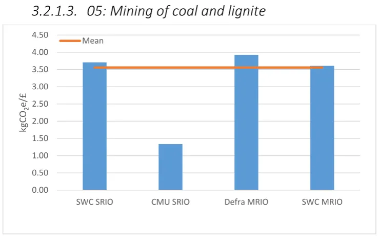
[image:32.595.131.501.70.304.2]

3.2.1.3. 05: Mining of coal and lignite

Figure 7 Comparison of carbon emissions factors for the mining of coal and lignite

There was significant disagreement between these models with a total range of 2.59 kgCO2e/£. As with the manufacture of iron and steel industry, the UK-based models broadly agreed for the mining of coal and lignite. Carnegie Mellon University calculated a much lower carbon emissions intensity that was more that 2 kgCO2e/£ less than the next lowest result. Defra calculated the greatest carbon factor for this industry at 3.93 kgCO2e/£.

The issues raised in the accuracy analysis of this industry sector regarding the impacts of multi-regional data may be partly responsible for this disagreement in precision analysis. The supply chain of mining of coal and lignite is quite simple, with 74% of the carbon emissions coming from the mining of coal and lignite sector, as this is an extractive industry. 11% of the carbon emissions for this sector come from the electricity production, transmission and distribution sector, which also has low agreement between models. This may have had some influence on the mining of coal and lignite industry model calculations.

0.00 0.50 1.00 1.50 2.00 2.50 3.00 3.50 4.00 4.50

SWC SRIO CMU SRIO Defra MRIO SWC MRIO

kgCO

2

e/£

(33)

32

[image:33.595.132.503.91.328.2]

3.2.1.4. 35.2-3: Gas; distribution of gaseous fuels through

mains; steam and air conditioning supply

Figure 8 Comparison of the carbon emissions factors for gas

Both of the multi-regional models calculated carbon emissions intensities above the mean of all models compared to the single-region models, both calculating values below the mean. The Defra value was the largest by a margin of 1.2 kgCO2e/£, with a total industry range between models of 1.7 kgCO2e/£. The single-region models agreed quite closely, only 0.05 kgCO2e/£ between them, however the specific reason was unclear. The Small World Consulting Ltd. single-region model was the most precise in this industry, calculating a value less than 7% from the mean of all models.

0.00 0.50 1.00 1.50 2.00 2.50 3.00 3.50

kgCO

2

e/£

(34)

33

[image:34.595.132.500.74.301.2]

3.2.1.5. 01: Agriculture

Figure 9 Comparison of carbon emissions factors for agriculture

The Small World Consulting Ltd. single-region model calculated, for agriculture, the most precise carbon emissions intensity with 0.03 kgCO2e/£ difference from the mean. The Carnegie Mellon University model again underestimated the mean significantly, whereas both multi-region models calculated estimates over the mean of models.

0.00 0.50 1.00 1.50 2.00 2.50 3.00 3.50 4.00

kgC

O2

e/£

(35)

34

[image:35.595.133.500.74.301.2]

3.2.1.6. 51: Air transport

Figure 10 Comparison of carbon emissions factors for air transport

For the air transport sector, the low agreement between models was most likely due to different assumptions within the calculations and methodology. The Small World Consulting Ltd. single-region model was an outlier in this industry sector. Their calculations simulated the highest value for the carbon intensity of the air transport industry; more than 1 kgCO2e/£ greater than the next nearest model. The lowest carbon intensity value was calculated by Carnegie Mellon University. This is likely at least partially due to the exclusion of a high-altitude factor from its methodology; however it is unclear if this accounts wholly for the disparity.

Within this industry the multi-regional models were the most precise with a range of 0.44 kgCO2e/£ between them, and the Defra model with a difference of only 0.03 kgCO2e/£ from the mean of all model estimates for the air transport sector. In this case, the Small World Consulting Ltd. single-region model calculated the largest estimate of 4.51 kgCO2e/£, 1.4 kgCO2e/£ larger than the Defra estimate and 2.87 kgCO2e/£ larger than the Carnegie Mellon University calculations.

0.00 0.50 1.00 1.50 2.00 2.50 3.00 3.50 4.00 4.50 5.00

kgC

O2

e/£

(36)

35

3.2.2. High Agreement Industry Sector Examples

The six industry sectors with the highest agreement were all service sectors. For this reason, only the three most precise service industry sectors were analysed. In addition to this, the three sectors from other industry types with the closest agreement were analysed for comparison. It should be kept in mind that high levels of agreement between models do not necessarily equate to accuracy of results.

[image:36.595.133.501.179.424.2]

3.2.2.1. 08: Other mining and quarrying products

Figure 11 Comparison of carbon emissions factors for other mining and quarrying products

Both of the Small World Consulting Ltd. models were the most precise in this industry as the single region-model calculated an emissions factor 0.03 kg CO2e/£ less than the mean of all models, and the multi-regional model calculated the same value greater than the mean. The Small World Consulting Ltd. single-region model was the only model to underestimate the carbon burden of this industry against the mean, whereas Defra overestimated compared to the mean most significantly. This suggests an influential role for multi-regional data inclusion.

0.00 0.10 0.20 0.30 0.40 0.50 0.60 0.70 0.80 0.90

kgC

O2

e/£

(37)

36

[image:37.595.135.499.76.312.2]

3.2.2.1. 41-43: Construction

Figure 12 Comparison of carbon emissions factors for construction

All UK-based models overestimated the mean of the construction industry, whereas the Carnegie Mellon University underestimated the mean. The Defra and Carnegie Mellon University models both disagreed with the mean by the same amount, though in different directions, potentially due to the difference in geographical background of the models or model structure, as the Carnegie Mellon University model disaggregates the construction industry into seven distinct industry sectors. The Small World Consulting Ltd. multi-regional model caluated the most precise carbon emissions factor.

Although the supply chain is reasonably diffuse among extractive and production industries for construction there is some reliance on the cement, lime, plaster and articles of concrete industry (11.7%) and the electricity production, transmission and distribution industry (21%). This may have some bearing on the findings in figure 12.

0.00 0.05 0.10 0.15 0.20 0.25 0.30 0.35 0.40 0.45 0.50

kgC

O2

e/£

(38)

37

[image:38.595.133.500.67.315.2]

3.2.2.2. 68.2IMP: Owner-

occupiers’ housing services

Figure 13 Comparison of carbon emissions factors for owner-occupiers' housing services

With only 0.05 kgCO2e/£ between the largest and smallest carbon intensity results for this industry sector it had the highest agreement of all industry sectors for the input-output models compared in this study. The multi-regional models both predicted the greatest values, and agreed extremely closely, down to the fifth decimal point, with Small World Consulting Ltd. providing the most precise calculation by a small margin. The Small World Consulting Ltd. single-region model also calculated a value very close to the mean of all models. The Carnegie Mellon University model disagreed most strongly as it underestimated the mean of all models by almost 0.04 kgCO2e/£, compared to the next largest disagreement with the mean at 0.01 kgCO2e/£.

42% of the supply chain for this industry is represented by the electricity production,

transmission and distribution industry sector and 14% represented by the air transport industry sector, both of which are low agreement industries. The high agreement nature of this industry is therefore likely due to something unrelated to those two industries.

0.00 0.01 0.02 0.03 0.04 0.05 0.06 0.07 0.08 0.09 0.10

kgC

O2

e/£

(39)

38

[image:39.595.135.500.74.313.2]

3.2.2.3. 49.1-2: Rail transport services

Figure 14 Comparison of carbon emissions factors for legal services

The total range of estimates for the carbon burden of the rail transport services industry was 0.25 kgCO2e/£. Defra’s carbon accounting model overestimated compared to the mean of all models by less than 0.003 kgCO2e/£ thus was extremely precise in representing this industry, followed in precision by the Small World Consulting Ltd. multi-regional model, suggesting a strong

methodological influence of multi-regional data inclusion. Both single region models were less precise, but in opposite kinds. This was possibly due to the methodological grounding. While 43% of the supply chain carbon burden for this industry is embodied in the rail transport sector itself, the other 57% is relatively diffuse thus the potential reasons for these findings are complex.

0.00 0.10 0.20 0.30 0.40 0.50 0.60 0.70 0.80 0.90

kgC

O2

e/£

An analysis of influential methodological practices in consumption based accounting methods

AN ANALYSIS OF

INFLUENTIAL

METHODOLOGICAL

PRACTICES IN

CONSUMPTION-BASED

ACCOUNTING METHODS

Acknowledgements

Declaration

Contents

Abstract

1.

Introductory material

1.1.

Literature and background

1.1.1.

Historical carbon accounting methods

1.1.2.

Input-output carbon accounting models

1.1.3.

Process-based life cycle assessments

1.1.4.

Hybrid carbon accounting methods

1.1.5.

Consumption-based accounting and the UK

1.1.6.

System boundary selection

1.2.

Aims and objectives

1.2.1.

Aims

1.2.2.

Objectives

2.

Methodology

2.1.

Input-Output Model Comparisons

2.1.1.

Input-output Model Mechanics

2.1.2.

Model Descriptions

2.1.2.1.

Carnegie Mellon University Environmental

Input-Output Life Cycle Assessment

2.1.2.2.

Department for Environment, Food and Rural

Affairs (Defra)

2.1.2.3.

Small World Consulting Ltd. Single-Region

Input-Output Model

2.1.2.4.

Small World Consulting Ltd. Multi-Regional Model

2.1.2.5.

Process-Based Life Cycle Assessments

2.1.2.6.

Important Notes

2.1.3.

Consumer Price Index Correction

2.1.4.

Accuracy Analysis

2.1.5.

Precision Analysis

2.2.

Copper Wire Case Study

2.2.1.

Argonne GREET.net model methodology

2.2.2.

Process-Based Life Cycle Analysis Methodology

2.2.3.

Gap Analysis

3.

Model Comparison Results

3.1.

Accuracy Analysis

3.1.1.

Confounded Analysis

3.1.2.

Unconfounded analysis

3.1.2.1.

Confounded and unconfounded analysis conclusion