Laura ++ : a Dalitz plot fitter

warwick.ac.uk/lib-publications

Original citation:

Back, J. J., Gershon, T. J., Harrison, Paul F., Latham, Thomas, O’Hanlon, Daniel, Qian, W., del

Amo Sanchez, Pablo, Craik, Daniel, Ilic, Jelena, Otalora Goicochea, Juan Martin, Puccio,

Eugenia, Silva Coutinho, Rafael and Whitehead, Mark (2018) Laura ++ : a Dalitz plot fitter.

Computer Physics Communications, 231. pp. 198-242. doi:10.1016/j.cpc.2018.04.017

Permanent WRAP URL:

http://wrap.warwick.ac.uk/103327

Copyright and reuse:

The Warwick Research Archive Portal (WRAP) makes this work of researchers of the

University of Warwick available open access under the following conditions.

This article is made available under the Creative Commons Attribution 4.0 International

license (CC BY 4.0) and may be reused according to the conditions of the license. For more

details see:

http://creativecommons.org/licenses/by/4.0/

A note on versions:

The version presented in WRAP is the published version, or, version of record, and may be

cited as it appears here.

Contents lists available atScienceDirect

Computer Physics Communications

journal homepage:www.elsevier.com/locate/cpc

Laura

++

: A Dalitz plot fitter

✩

John Back

a

, Tim Gershon

a

, Paul Harrison

a

, Thomas Latham

a,

*

, Daniel O’Hanlon

a,1

,

Wenbin Qian

a

, Pablo del Amo Sanchez

b

, Daniel Craik

c

, Jelena Ilic

d

,

Juan Martin Otalora Goicochea

e

, Eugenia Puccio

f

, Rafael Silva Coutinho

g

,

Mark Whitehead

h,2

a_{Department of Physics, University of Warwick, Coventry, United Kingdom} b_{LAPP, Université Savoie Mont-Blanc, CNRS/IN2P3, Annecy-Le-Vieux, France}

c_{Massachusetts Institute of Technology, Cambridge, USA}

d_{STFC Rutherford Appleton Laboratory, Didcot, United Kingdom}

e_{Universidade Federal do Rio de Janeiro (UFRJ), Rio de Janeiro, Brazil}

f_{Stanford University, Stanford, USA}

g_{Physik-Institut, Universität Zürich, Zürich, Switzerland}

h_{European Organization for Nuclear Research (CERN), Geneva, Switzerland}

a r t i c l e i n f o

Article history:

Received 19 January 2018

Received in revised form 22 January 2018 Accepted 2 April 2018

Available online 2 May 2018

Keywords:

Event reconstruction and data analysis Dalitz plot

Amplitude analysis Isobar model

K-matrix Flavour physics

a b s t r a c t

The Dalitz plot analysis technique has become an increasingly important method in heavy flavour physics. The Laura++ fitter has been developed as a flexible tool that can be used for Dalitz plot analyses in different experimental environments. Explicitly designed for three-body decays of heavy-flavoured mesons to spinless final state particles, it is optimised in order to describe all possible resonant or nonresonant contributions, and to accommodate possibleCPviolation effects.

Program summary Program title:Laura++

Program Files doi:http://dx.doi.org/10.17632/jn266r57nk.1 Licensing provisions:Apache License, Version 2.0

Programming language:C++

Nature of problem: Dalitz-plot analysis of particle decays is an important and increasingly utilised technique in particle physics, in particular in heavy flavour physics. While various software tools have been used for Dalitz plot analyses, these are usually not well optimised and are neither scalable for use with larger samples nor flexible enough to be easily adapted for other analyses.

Solution method:Laura++ is a dedicated package for performing Dalitz-plot analysis that is flexible enough both to be used in a range of experimental environments and to describe many possible different decays and types of analyses. It allows analysts to create amplitude models to describe the decay of interest and to use those models either to generate pseudoexperiments or to fit them to data.

©2018 The Author(s). Published by Elsevier B.V. This is an open access article under the CC BY license (http://creativecommons.org/licenses/by/4.0/).

1. Introduction

Decays of unstable heavy particles to multibody final states can in general occur through several different intermediate resonances. Each decay channel can be represented quantum-mechanically by an amplitude, and the total density of decays across the phase space is represented by the square of the coherent sum of all contributing amplitudes. Interference effects can lead to excesses or deficits of decays in regions of phase space where different resonances overlap. Investigations of such dynamical effects in multibody decays are of great interest to test the Standard Model of particle physics and to investigate resonant structures.

✩_{This paper and its associated computer program are available via the Computer Physics Communication homepage on ScienceDirect (http://www.sciencedirect.com/}

science/journal/00104655).

*

Corresponding author.

E-mail address:[email protected](T. Latham).

1_{Now at Sezione INFN di Bologna, Bologna, Italy.}

2_{Now at I. Physikalisches Institut, RWTH Aachen University, Aachen, Germany.}

https://doi.org/10.1016/j.cpc.2018.04.017

[image:3.595.95.513.53.300.2]

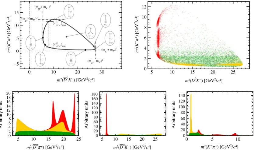
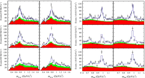
Fig. 1.(Top left) kinematic boundaries of the three-body phase space for the decayB0 s→D

0

K−_π+_{. The insets indicate the configuration of the final-state particle momenta}

in the parent rest frame at various different DP positions. (Top right) examples of the resonances which may appear in the Dalitz plot for this decay: (red)D∗ s2(2573)

−

, (orange)

K∗₍₈₉₂₎0_{, (green)KπS-wave. (Bottom) projections of this DP onto the squares of the invariant masses (from left to right):m}2

D0π+,m

2

D0K−,m

2

K−_π+. (For interpretation of the

references to colour in this figure legend, the reader is referred to the web version of this article.)

The Dalitz plot (DP) [1,2] was introduced originally to describe the phase space ofK_L0

→

πππ

decays, but is relevant for the decay of any spin-zero particle to three spin-zero particles,P

→

d1d2d3. In such a case, energy and momentum conservation give

m2_P

+

m2_d1

+

m_d2₂

+

m2_d3

=

m2(d1d2)

+

m2(d2d3)

+

m2(d3d1)

,

(1)

wherem(didj) is the invariant mass obtained from the two-body combination of thedi anddjfour momenta. Consequently, assuming

that the masses ofP,d1,d2andd3are all known, any two of them2(didj) values – subsequently referred to as Dalitz-plot variables – are

sufficient to describe fully the kinematics of the decay in thePrest frame. This can also be shown by considering that the 12 degrees of freedom corresponding to the four-momenta of the three final-state particles are accounted for by two DP variables, the threedimasses,

four constraints due to energy–momentum conservation in theP

→

d1d2d3decay, and three co-ordinates describing a direction in space

which carries no physical information about the decay since all particles involved have zero spin.

A Dalitz plot is then the visualisation of the phase space of a particular three-body decay in terms of the two DP variables.3 Analysis of the distribution of decays across a DP can reveal information about the underlying dynamics of the particular three-body decay, since the differential rate is

dΓ

=

1

(2

π

)3

1

32m3_P

|

A

|

2_dm2_(d

1d3)dm2(d2d3)

,

(2)

whereAis the amplitude for the three-body decay. Thus, any deviation from a uniform distribution is due to the dynamical structure of the amplitude. Examples of the kinematic boundaries of a DP, and of resonant structures that may appear in this kind of decay, are shown inFig. 1.

The Dalitz-plot analysis technique, usually implemented with model-dependent descriptions of the amplitudes involved, has been used to understand hadronic effects in, for example, the

π

0

π

0

π

0system produced inpp

¯

annihilation [3]. Recently, it has also been used to study three-body

ηc

decays [4,5]. However, DP analyses have become particularly popular to study multibody decays of the heavy-flavouredD

andBmesons. Not only do the relatively large masses of these particles provide a broad kinematic range in which resonant structures can be studied but, since the decays are mediated by the weak interaction, there may beCP-violating differences between the DP distributions for particle and antiparticle. Studying these differences can test the Standard Model mechanism forCPviolation: if the asymmetries are not consistent with originating from the single complex phase in the Cabibbo–Kobayashi–Maskawa (CKM) quark mixing matrix [6,7] then contributions beyond the Standard Model must be present.

Until around the year 2000, most DP analyses of charm decays were focussed on understanding hadronic structures at low

ππ

orK

π

mass. In particular, pioneering analyses ofD

→

K

ππ

decays were carried out by experiments such as MARK-II, MARK-III, E687, ARGUS, E691 and CLEO [8–13]. These analyses revealed the existence of a broad structure in theK

π

S-wave that could not be well described with a Breit–Wigner lineshape. In later analyses, it was shown that this contribution could be modelled in a quasi-model-independent way, in which the partial wave is fitted using splines to describe the magnitude and phase as a function ofm(K

π

) [14]. Subsequent uses of

3_{The phrase ‘‘Dalitz plot’’ is often used more broadly in the literature. In particular, it can be used to describe the projection onto two of the two-body invariant mass}

this approach include further studies of theK

π

S-wave [5,15–17] as well as theK+

K−

[18] and

π

+

_π

−

[19] S-waves, in various processes. Similarly, DP analyses of decays such asD+

_→

_π

+

_π

+

_π

−

[20–23] indicated the existence of a broad low-mass

ππ

S-wave known as the

σ

pole [24].

With the advent of thee+

e−

B-factory experiments, BaBar [25,26] and Belle [27], DP analyses ofBmeson decays became feasible. The method was used to obtain insights into charm resonances through analyses ofB+

→

D−

π

+

π

+[28,29] andB0

→

D0

π

+

π

−[30,31] decays. Studies ofBmeson decays to final states without any charm or charmonium particles also became possible [32–34]. Once baseline DP models were established, it was then possible to search forCPviolation effects, with results including the first evidence forCPviolation in theB+

_→

_ρ

(770)0_K+

decay [35,36]. Moreover, analyses that accounted for possible dependence of theCPviolation effect with decay time as well as with DP position were carried out for bothD[37,38] andBdecays [39–46].

With the availability of increasingly large data samples at these experiments and, more recently, at the Large Hadron Collider experiments (in particular, LHCb [47]), more detailed studies of these and similar decays become possible. In addition, many ideas for DP analyses have been proposed, since they provide interesting possibilities to provide insight into hadronic structures, to measureCP

violation effects and to test the Standard Model. These include methods to determine the angles

α

,

β

and

γ

of the CKM Unitarity Triangle with low theoretical uncertainty from, respectivelyB0

_→

_π

+

_π

−

_π

0_[48],B0

_→

_D

_π

+

_π

−

[49,50] andB0

_→

_DK+

_π

−

decays [51,52], among many other potential analyses.

Thus, it has become increasingly important to have a publicly available Dalitz-plot analysis package that is flexible enough both to be used in a range of experimental environments and to describe many possible different decays and types of analyses. Such a package should be well validated and have excellent performance characteristics, in particular in terms of speed since complicated amplitude fits can otherwise have unacceptable CPU requirements. This motivated the creation, and ongoing development, of theLaura++ package, which is described in the remainder of the paper.Laura++is written in theC++programming language and is intended to be as close as possible to being a standalone package, with a sole external dependency on theRootpackage [53]. In particular,Rootis used to handle data file input/output, histogrammed quantities, and the minimisation of negative log-likelihood functions withMinuit[54]. Further documentation and code releases (distributed under the Apache License, Version 2.0 [55]) are available fromhttp://laura.hepforge.org/.

The description of the software given in this paper corresponds to that released inLaura++version

v3r4

.

In Section2, a brief summary of the Dalitz-plot analysis formalism is given, and the conventions used inLaura++are set out. Section3

describes effects that must also be taken into account when performing an experimental analysis. Sections4–6then contain discussions of, respectively, the implementation of the signal model, efficiency and resolution effects, and the background components inLaura++,

including explicit classes and methods with high-level details given in Appendices. These elements are then put together in Section7, where the overall work flow inLaura++is described. The performance of the software is discussed in Section8, ongoing and planned

future developments are briefly mentioned in Section9, and a summary is given in Section10.

2. Dalitz-plot analysis formalism

Given two variables that describe the Dalitz plot of theP

→

d1d2d3decay, all other kinematic quantities can be uniquely determined

for fixed initial- and final-state (subsequently referred to as parent and daughter) particle masses. The convention adopted inLaura++is that the DP is described in terms ofm2₁₃

≡

m2(d1d3) andm223

≡

m

2_(d

2d3). Hence, these two variables are required to be present in any

input data provided toLaura++.

The description of the complex amplitude is based on the isobar model [56–58], which describes the total amplitude as a coherent sum ofNamplitudes from resonant or nonresonant intermediate processes.4 _{This means that the total amplitude is given by}

A

(

m2₁₃

,

m2₂₃

)

=

N

∑

j=1 cjFj

(

m2₁₃

,

m2₂₃

)

,

(3)

wherecjare complex coefficients, discussed further in Section4.5, giving the relative contribution of decay channelj. There are several

different choices used in the literature to express the resonance dynamics contained within theFj

(

m2₁₃

,

m2₂₃

)

terms. Here, one common approach, which is the default inLaura++, is outlined; other possibilities are discussed inAppendices AandB. For a resonance inm13, the

dynamics can be written as

F

(

m2₁₃

,

m2₂₃

)

=

N

×

R

(

m13

)

×

T(p

⃗

,

⃗

q)

×

X(

|⃗

p

|

rBWP )

×

X(

|⃗

q

|

rBWR )

,

(4)

where the functionsRandTdescribe the invariant mass and angular dependence of the amplitude, theXfunctions are form factors, and

N is a normalisation constant. In Eq.(4)only the kinematic – i.e. DP – dependence has been specified; the functions may also depend on properties of the resonance such as mass, width and spin. The arguments

⃗

qandp

⃗

are the momentum of one of the resonance decay products (d3in this case, see Section2.4for further information) and that of the so-called ‘‘bachelor’’ particle (i.e. the particle not associated

with the decay of the resonance;d2in this case), both evaluated in the rest frame of the resonance. The parametersrBWP andrBWR are

characteristic meson radii described below. The resonance dynamics are normalised inLaura++such that the integral over the DP of the

squared magnitude of each term is unity

∫ ∫

DP

⏐

⏐

F_j

(

m2₁₃

,

m2₂₃

)⏐

⏐

2

dm2₁₃dm2₂₃

=

1

.

(5)

Although not strictly necessary, as only the total probability density function (PDF) needs to be normalised, this allows a meaningful comparison of the values of thecjcoefficients.

4_{Alternative descriptions of parts of the amplitude model are also available inLaura}++

2.1. Resonance lineshapes

In Eq.(4), the function R

(

m13

)

is the resonance mass term. The detailed forms for all available shapes inLaura

++

are given in

Appendix A. Here the most commonly used relativistic Breit–Wigner (RBW) lineshape is given as an example

R(m)

=

1

(m2

0

−

m2)

−

i m0Γ(m)

,

(6)

wherem0is the nominal mass of the resonance and the dependence of the decay width of the resonance onmis given by

Γ(m)

=

Γ₀

(

q q0

)

2L+1

(

m₀

m

)

X2(q r_BWR )

,

(7)

whereΓ0is the nominal width of the resonance andq0denotes the value ofqwhenm

=

m0. In Eq.(7),Lis the orbital angular momentum

between the resonance daughters. Note that since all the initial- and final-state particles have zero spin, this quantity is the same as the spin of the resonance and is also the same as the orbital angular momentum between the resonance and the bachelor.

It is relevant to note that Eq.(6)can be written

m0Γ(m)R(m)

=

m0Γ(m)

(m2

0

−

m2)

−

i m0Γ(m)

≡

sin

φ

expi

φ ,

(8)

where tan

φ

=

m0Γ(m)

m2 0−m2

. This shows the characteristic phase rotation of a resonance asm2increases from far below to far abovem2₀.

2.2. Angular distributions and Blatt–Weisskopf form factors

Using the Zemach tensor formalism [59,60], the angular probability distribution termsT(

⃗

p

,

⃗

q) are given by

L

=

0

:

T(

⃗

p

,

⃗

q)

=

1

,

(9)

L

=

1

:

T(

⃗

p

,

q

⃗

)

= −

2p

⃗

· ⃗

q

,

(10)

L

=

2

:

T(

⃗

p

,

⃗

q)

=

4

3

[

3(

⃗

p

· ⃗

q)2

−

(p q)2

]

,

(11)

L

=

3

:

T(

⃗

p

,

⃗

q)

= −

24

15

[

5(

⃗

p

· ⃗

q)3

−

3(p

⃗

· ⃗

q)(p q)2

]

,

(12)

L

=

4

:

T(

⃗

p

,

⃗

q)

=

16

35

[

35(

⃗

p

· ⃗

q)4

−

30(

⃗

p

· ⃗

q)2(p q)2

+

3(p q)4

]

,

(13)

L

=

5

:

T(

⃗

p

,

⃗

q)

= −

32

63

[

63(

⃗

p

· ⃗

q)5

−

70(

⃗

p

· ⃗

q)3(p q)2

+

15(

⃗

p

· ⃗

q)(p q)4

]

,

(14)

whereq

≡ |⃗

q

|

andp

≡ |⃗

p

|

. These have the form of the Legendre polynomialsPL(cos

θ

), where

θ

is the ‘‘helicity’’ angle betweenp

⃗

and

⃗

q,

multiplied by the appropriate power of

−

2p q. These factors act to suppress the amplitude at low values of the break-up momentum in either the decay of the parent or the resonance — the so-called ‘‘angular momentum barrier’’. However, these factors on their own would cause the amplitude to continue to grow with increasing break-up momentum even once the barrier was exceeded. The termsX(z), where

z

=

p rP

BWorq rBWR , are Blatt–Weisskopf form factors [61], which act to cancel this behaviour once above the barrier. They are given by

L

=

0

:

X(z)

=

1

,

(15)

L

=

1

:

X(z)

=

√

1

+

z2

0

1

+

z2

,

(16)

L

=

2

:

X(z)

=

√

z₀4

+

3z₀2

+

9

z4

₊

_3z2

₊

₉

,

(17)

L

=

3

:

X(z)

=

√

z₀6

+

6z₀4

+

45z₀2

+

225

z6

₊

_6z4

₊

_45z2

₊

₂₂₅

,

(18)

L

=

4

:

X(z)

=

√

z8

0

+

10z06

+

135z04

+

1575z02

+

11025

z8

₊

_10z6

₊

_135z4

₊

_1575z2

₊

₁₁₀₂₅

,

(19)

L

=

5

:

X(z)

=

√

z10

0

+

15z08

+

315z06

+

6300z04

+

99225z02

+

893025

z10

₊

_15z8

₊

_315z6

₊

_6300z4

₊

_99225z2

₊

₈₉₃₀₂₅

,

(20)

wherez0represents the value ofzwhenm

=

m0. The radius of the barrier, denotedrBWP orr

R

BWwhere the superscript indicates that the

2.3. Fit fractions

In the absence of any reconstruction effects, the DP PDF would be

Pphys

(

m2₁₃

,

m2₂₃

)

=

⏐

⏐

A

(

m2 13

,

m223

)⏐

⏐

2

∫∫

DP

⏐

⏐

A

(

m2₁₃

,

m2₂₃

)⏐

⏐

2

dm2₁₃dm2₂₃

.

(21)

In a real experiment, the variation of the efficiency across the DP and the contamination from background processes must be taken into account; these details are discussed in Sections3,5and6.

Typically, the primary results – i.e. the values obtained directly in the fit to data – of a DP analysis include the complex amplitude coefficients, given bycjin Eq.(3), that describe the relative contributions of each intermediate process. These results are dependent on

a number of factors, including the amplitude formalism, choice of normalisation and phase convention used in each DP analysis. This makes it difficult to make useful comparisons between complex coefficients obtained from different analyses using different software. Fit fractions provide a convention-independent method to make meaningful comparisons of results from different fits. The fit fraction is defined as the integral of a single decay amplitude squared divided by that of the coherent matrix element squared for the complete DP,

FFj

=

∫∫

DP

⏐

⏐

cjFj

(

m2 13

,

m223

)⏐

⏐

2 dm2

13dm223

∫∫

DP

⏐

⏐

A

(

m2 13

,

m223

)⏐

⏐

2 dm2

13dm223

.

(22)

The sum of these fit fractions is not necessarily unity due to the potential presence of net constructive or destructive interference. Such effects can be quantified by defining interference fit fractions (fori

<

jonly) as

FFij

=

∫∫

DP2 Re

[

cicj∗Fi

(

m2 13

,

m223

)

F∗

j

(

m2 13

,

m223

)]

dm2 13dm223

∫∫

DP

⏐

⏐

A

(

m2 13

,

m223

)⏐

⏐

2 dm2

13dm223

.

(23)

The interference fit fractions describe the net interference between the amplitudes of two intermediate processes. Interference effects between different partial waves in a given two-body combination cancel when integrated over the helicity angle. Therefore, non-zero interference fit fractions should arise only between contributions in the same partial wave of one two-body combination, or between contributions in different two-body combinations. Large interference fit fractions, or equivalently a sum of fit fractions very different from unity, can often be an indication of inadequate modelling of the Dalitz plot.

2.4. Helicity angle convention

In the formalism just described, there is a choice as to which of the two resonance daughters the momentum

⃗

qshould be attributed (and hence to attribute the momentum

−⃗

qto the other). This choice, although arbitrary, will affect the values of the measured phases and hence it is important that it is documented to allow comparisons between results. The convention used inLaura++is as follows:

•

θ

₁₂is defined as the angle betweend1andd3in the rest frame of thed1andd2system, i.e.

⃗

qis the momentum ofd1;

•

θ

₂₃is defined as the angle betweend3andd1in the rest frame of thed2andd3system, i.e.

⃗

qis the momentum ofd3;

•

θ

₁₃is defined as the angle betweend3andd2in the rest frame of thed1andd3system, i.e.

⃗

qis the momentum ofd3.

This convention is illustrated inFig. 2. One important point to note is that it is not a cyclic permutation. Rather it is designed such that for decays whered1andd2are identical particles the formalism is already symmetric under their exchange, as required.

For decays of neutral particles to flavour-conjugate final states containing two charged daughters, e.g.

(—)

B

→

π

+

_π

−

K0

S, there is a further

complication that must be considered. In the example given, if one chooses for theBdecay thatd1would be

π

+

,d2would be

π

− andd3

would beK_S0, one should then define theBdecay using the conjugate particles, i.e.d1would be

π

−,d2would be

π

+andd3would be K0

S. In practice, however, one often has an untagged data sample that contains bothBandBdecays that are not distinguished and so a

single definition of the DP must be used. (Flavour-tagged analyses are discussed in Section9.) Consequently, the amplitude model must account for the incorrect particle assignments for one of the flavours. Due to the choice of convention inLaura++this can be handled in a straightforward manner as long as the self-conjugate particle (theK_S0in the example given) is assigned to bed3. Under these circumstances,

the relationF

(

m2 13

,

m223

)

=

F

(

m2 23

,

m213

)

can be restored simply by multiplying by

−

1 the cosine of the helicity angle

θ

12in the amplitude

calculations for either the particle or antiparticle decay — we choose to do this for the particle decay (theBdecay in the example given). So, in the considered example, a contribution fromB0

→

ρ

(770)0K_S0would have its helicity angle definition inverted with respect to that ofB0

→

ρ

(770)0_K0

S.

3. Experimental effects

In order to extract physics results from reconstructedP

→

d1d2d3candidates using real experimental data, several effects need to

be taken into account. One major concern will be that any backgrounds that fake the signature of signal decays need to be removed, which is usually done by imposing various selection criteria that exploit differences in the kinematics and topologies between signal and background events.

The effect of applying selection criteria invariably means that the probability of reconstructing signal decays will not be 100% and furthermore could vary as a function of DP position. Along the boundaries, at least one of the daughter particles has low momentum, which typically reduces the reconstruction efficiency compared to decays at or near the DP centre. To account for this effect properly, the signal PDF, originally defined in Eq.(21), needs to be modified to

Psig

(

m2₁₃

,

m2₂₃

)

=

⏐

⏐

A

(

m2₁₃

,

m2₂₃

)⏐

⏐

2

ϵ

(

m2₁₃

,

m2₂₃

)

∫∫

DP

⏐

⏐

A

(

m2 13

,

m223

)⏐

⏐

2

ϵ

(

m2 13

,

m223

)

dm2 13dm223

[image:7.595.81.530.52.175.2]

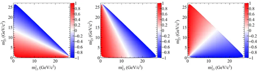
Fig. 2.Values of the cosine of the helicity angles (left)θ13, (middle)θ23, and (right)θ12as functions of DP position. The kinematic boundary of this DP corresponds to that for

theB0→π+_π−_π0_decay.

where the signal efficiency

ϵ

(

m2 13

,

m223

)

is defined as the fraction of signal decays at the given DP position that are retained after all selection criteria have been applied.

For certain modes, there can be decay channels that can mimic the properties of the signal mode under study. For example, there may be significant backgrounds to the charmless decay B−

_→

K−

_π

+

_π

−

from the decay modesB−

_→

D0

π

−

_,

D0

→

K−

_π

+ or

B−

→

χc

₀K−

, χc

0

→

π

+

π

−

. Such backgrounds can be removed, or at least suppressed, by applying a ‘‘veto’’, which means excluding candidates that lie within, typically, three to five widths on either side of the mass peak. Alternatively, they can be accounted for within the signal model.

Another issue that needs to be considered is the effect of finite experimental resolution in the determination of the momentum of the parentPand its daughter particles. This leads to imperfect measurements of the invariant mass-squared combinations of the daughters, and also causes uncertainty on the invariant mass of the reconstructedPcandidate. To avoid creating a DP with a fuzzy boundary, the mass ofPcan be fixed to its expected value, with adjustments made to the four-momenta of its daughter particles to ensure momentum–energy conservation. This will in general improve the resolution of the measurement of the DP co-ordinates, however there may still be significant effects related to events migrating from one region of the DP to another, especially near the corners of the kinematic boundary. This effect is usually ignored if the size of the migration/resolution is smaller than the width of the narrowest resonance under consideration, or if the largest migration probability is below 10% or so (although in the latter case, it is likely that systematic uncertainties on the physics results would need to be evaluated). If particularly narrow resonances contribute to the decay or if the final state particles under study suffer from significant misreconstruction effects (as is often the case for decays involving neutral pions), these effects can be taken into account rather generically by adding a ‘‘self cross-feed’’ component to the signal PDF. In this component, the true PDF is smeared by the resolution function

w

scf(sreco

,

strue), given in terms of the reconstructed and true DP positionssreco

≡

(m213

,

m

2

23) andstrue. The total signal

PDF is then

P_sig-scf(sreco)

= [

1

−

fscf(sreco)

]

Psig(sreco)

+

∫

fscf(strue)

w

scf(sreco

,

strue)Psig(strue)dstrue

,

(25)

where for the first component the resolution is negligible (equivalent to

w

scf being a delta function), and the level of the second

is determined by the self cross-feed fraction fscf(strue), i.e. the fraction of reconstructed events with true DP position strue that are

misreconstructed. The integral is over all true DP positions, although in practice only those with non-zero values of

w

scffor the given sreconeed to be included. The fractionfscfcan vary between 0 and 1, which correspond to the cases that resolution is negligible or that it

must be considered for all signal events. The map

w

scfis sufficiently flexible to account for the fact that resolution may be more important

to consider in some regions of the DP than others.

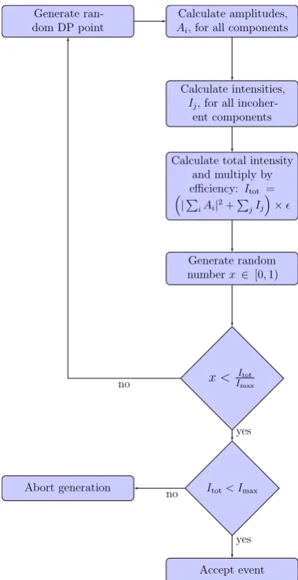
Despite imposing selection requirements in order to select signal candidates, there can remain significant fractions of various backgrounds in the DP analysis sample. This means that an extended likelihood functionLneeds to be employed in order to include these additional contributions:

L

=

e−N

Nc

∏

j

[

∑

k

NkPkj

]

,

(26)

whereNis equal to

∑

kNk,Nkis the yield for the event categoryk(signal or background),Ncis the total number of candidates in the data

sample, andP_kjis the PDF for the categorykfor eventj, which consists of the product of the DP PDF and any other (uncorrelated) PDFs that are used to discriminate between signal and background. The function

−

2 lnLis minimised in an unbinned fit to the data in order to extract all of the parameters.

4. Implementation of the signal component

In this section we begin to describe the code structure of theLaura++package by first outlining the classes and methods used to build up the total DP amplitude of the signal, given in Eq.(3). Furthermore, we describe how this is normalised in order to form the signal PDF defined in Eq.(21).

4.1. Particle definitions and kinematics

The most fundamental parts of the code define the properties of the parent particlePand its three daughtersd1,d2andd3and their

associated kinematics. Allowed types forPareB+ ,B−

,B0_,B0_,B0 s,B

0 s,D

+ ,D−

,D0_,D0_,D+

s andD

−

s, while the possible daughters types are

π

+ ,

π

−

,

π

0,K+ ,K−

,K_S0,

η

,

η

′ ,D+

,D−

,D0,D0,D+

s andD

−

s.5 The information on the decay that is to be modelled is encapsulated within the

LauDaughters

class, which is constructed by providing the names or PDG codes [62] of the parent and daughters. The particle properties are retrieved using the

LauDatabasePDG

singleton class, which extracts and supplements information from theRoot

TDatabasePDG

particle property class.

The

LauDaughters

object then instantiates a

LauKinematics

instance, supplying to it the masses of the parent and its daughters. Instances of

LauKinematics

are used throughout theLaura++code to calculate and store all of the required kinematic variables for a given position in the DP (usually supplied asm2

13andm223). These kinematic variables include the two-body invariant masses and helicity

angles, the momenta of the daughters in the parent rest frame and in each of the two-body rest frames. In addition, there is the option to calculate the co-ordinates of the so-called ‘‘square Dalitz plot’’.

4.1.1. Square Dalitz plot

Since, particularly inBdecays, signal events tend to populate regions close to the kinematic boundaries of the DP, it can be convenient to use a co-ordinate transformation into the so-called square Dalitz plot (SDP) [33]. The SDP is defined by variablesm′

and

θ

′

that have validity ranges between 0 and 1 and are given by

m′

≡

1

π

cos

−1

(

2m12

−

m

min 12 mmax₁₂

−

mmin₁₂

−

1

)

and

θ

′

≡

1

π

θ

12

,

(27)

wheremmax₁₂

=

mP

−

md3andm min

12

=

md1

+

md2are the kinematic limits ofm12allowed in theP

→

d1d2d3decay, while

θ

12is the helicity

angle betweend1andd3in thed1d2rest frame, as explained in Section2.4. Similar to how a choice of DP variables must be made, the SDP

can be defined in several different ways. The expressions of Eq.(27)correspond to the choice used inLaura++, which must be employed

consistently whenever a SDP is used.

To transform between DP and SDP representations, it is necessary to ensure correct normalisation. This is achieved by including the determinant of the Jacobian of the transformation, which is given by

|

J

| =

4p q m12

∂

m12

∂

m′

∂

cos

θ

12

∂θ

′

,

(28)

wherepandqare evaluated in thed1d2rest frame and the partial derivatives evaluate to

∂

m12

∂

m′

= −

π

2sin(

π

m ′

)

(

mmax₁₂

−

mmin₁₂

)

,

∂

cos

θ

12

∂θ

′

= −

π

sin(

πθ

′

)

.

(29)

The SDP coordinate system has several advantages that apply whenever there is a need to bin the phase space, which are illustrated inFig. 3. Firstly, the regions near the kinematic boundary are spread out, which means that these regions where the signal is often concentrated and where also there can be rapid variation in efficiency and background distributions can be treated with a much finer resolution, even while maintaining a uniform binning. Secondly, the kinematic boundary is perfectly aligned with the bin edges.

4.2. Isobar dynamics and resonances

Once the kinematics of a particular decay mode have been established, the structure of the signal DP model can be by defined by creating a

LauIsobarDynamics

object. Components of the model are specified using the

addResonance

member function, which requires:

•

the name of the resonance,

•

an integer that specifies which of the daughters is the bachelor particle, and hence in which invariant mass spectrum this resonance will appear (1 form23, 2 form13, 3 form12or 0 for some nonresonant models),

•

an enumeration to select the form of the dynamical amplitude.

Appendix C contains lists of the names of the allowed resonances along with their nominal mass, width, spin, charge and Blatt– Weisskopf barrier radius. This information is all automatically retrieved from

LauResonanceInfo

records that are stored in the

LauResonanceMaker

class.Appendix Calso provides information on how to account for a state that is not already included inLaura++,

and how to change the nominal values of the properties of any resonance.Appendix Agives details of all the dynamical amplitude forms that are currently implemented in the package and inTable A.1supplies the corresponding enumeration types. Examples of usage are given in Section7.1.

Fig. 3. Illustration of the transformation between conventional and square Dalitz plot representations, for resonances in theB0

s →D

0

π+ K−

decay (here the final-state particles are ordered following thed1d2d3convention ofLaura++). Compared to the same DP shown inFig. 1, a fakeD0π+

resonance, with parameters corresponding to those of theD∗

2(2460)

+

state (blue points) has been added in order to better visualise the transformation in relevant DP regions. (For interpretation of the references to colour in this figure legend, the reader is referred to the web version of this article.)

The signal model may also include contributions that do not interfere with the other resonances in the DP. These may arise due to decays that proceed via intermediate long-lived, i.e. negligible natural width, states; an example is the contribution fromB−

_→

D0

_π

− ,

D0

_→

_K−

π

+ inB−

→

K−

π

+

π

−

decays. Experimentally, such components can be considered either as signal or background, and selection requirements (e.g., based on the consistency of the three daughter tracks of originating from the same vertex position) may be used to suppress them, but in certain cases some contribution will remain. WithinLaura++, the user can choose how to treat such contributions. When considered as part of the signal model, non-interfering components can be added with the

addIncoherentResonance

member function, which has the same number and type of arguments as the

addResonance

function. In this case the form of the dynamical amplitude should be specified as

GaussIncoh

, and the width should be changed to correspond to the experimental resolution. Note that the resolution for incoherent contributions is handled in a different way to the approach described in Sections3and5.2. As part of the signal model, a non-interfering component will contribute to the denominator of the fit fractions, but it is simple for the user to subtract it from the results since there is no interference with other components.

When building the model,Laura++ performs a simple check of charge conservation, while angular momentum is conserved by construction. However, the onus is on the user to make sure that the strong decays of resonances included in the model respect conservation of parity and flavour quantum numbers, since these are not checked by the code. In order to help with this, a summary of all resonances used in the model is printed out during the initialisation.

The complex dynamical amplitudesR(m) of the various resonance forms are defined using classes that inherit from the abstract base class

LauAbsResonance

. For example, the relativistic Breit–Wigner lineshape is defined within the

LauRelBreitWignerRes

class. All such classes implement the

resAmp

member function that returns a

LauComplex

class that represents the amplitude at the given value of the relevant two-body invariant mass. The

LauAbsResonance

base class implements the calculation of the angular distribution factor. Those amplitude forms that require the calculation of the Blatt–Weisskopf factors make use of the

LauBlattWeisskopfFactor

helper class.

4.3. Symmetry

If the decay ofPcontains two identical daughters, such as inB+

→

π

+

π

+

π

−, then the DP will be symmetric. As mentioned in Section2.4, the identical particles should be positioned asd1andd2. This situation is automatically detected by

LauDaughters

and the

information propagated to the amplitude model. In this case, it is required only to define the resonances for the paird1d3; the amplitude

is automatically symmetrised by

LauIsobarDynamics

by flipping the invariant-mass squared variablesm2

13

↔

m223, recalculating the

amplitude and summing.

When all of the daughters are identical, for example inB0

_→

_K0

SKS0KS0, it is again only needed to define the resonances for one of

the pairs (usuallyd1d3). For this fully symmetric case,

LauIsobarDynamics

automatically performs the necessary symmetrisation of

the amplitude by cyclically rotating the invariant-mass squared variables (m2₁₂

→

m2₂₃,m2₂₃

→

m2₁₃,m2₁₃

→

m2₁₂) and flipping them (m2₁₃

↔

m2₂₃).

4.4. Normalisation of signal model

Various integrals of the dynamical amplitude across the DP need to be calculated in order to normalise the signal PDF given by Eq.(21), as well as for calculating the fit fractions for individual resonances defined in Eqs.(22)and(23). Since thecjcoefficients are constant

across the DP, only the amplitude termsFjneed to be integrated. In general, these integrals cannot be found analytically, so Gauss–Legendre

quadrature is used to evaluate them numerically. This is achieved by dividing the DP into an unequally spaced grid whose points correspond to the abscissa co-ordinates from the quadrature procedure. The granularity of the grid is chosen to ensure sufficiently precise integration, as discussed in more detail below. TheFjterms are then multiplied by the quadrature weights and summed over all grid points that lie

is replaced bydm13dm23multiplied with the Jacobian factor 4m13m23. This means that the normalisation of the total amplitudeAis given

by

∫ ∫

DP

|

A

|

2dm2₁₃dm2₂₃

≈

Na

∑

a=1

Nb

∑

b=1

4hahbwawb

|

A

|

2

,

(30)

where

wa

(

wb

) are the weights for the Gauss–Legendre quadrature abscissa valuesha(hb), which correspond to the grid points along the

m13(m23) axis, and the amplitudeAis evaluated for all abscissas inside the DP kinematic boundary. An equivalent expression is used for

normalisation of the experimental signal PDF of Eq.(24). The number of pointsNa(Nb) is set by dividing them13(m23) mass range by a

default ‘‘bin width’’

δ

mof 5 MeV

/

c2_{, which can be changed using the}

_{setIntegralBinWidths}

_{function in}

_{LauIsobarDynamics}

_{, giving}

∼

1000 integration bins along each mass axis forBdecays. It is important to realise that

δ

mis not, in general, equal to the separation between neighbouring abscissa points. The

LauIntegrals

class handles the calculation of the general weights and abscissas for the integration range (

−

1

,

1), while the

LauDPPartialIntegralInfo

class scales these using the half-ranges and mean values ofm13and m23, following the numerical recipe given in Ref. [63]. This information is then used within the

LauIsobarDynamics

class to find the

normalisation integral for the total amplitude, as well as the integrals for the fit fractions.

If the DP contains narrow resonances with widths below a threshold value, which defaults to 20 MeV

/

c2_{but can be changed using the}

setNarrowResonanceThreshold

function in

LauIsobarDynamics

, then the quadrature grid is split up into smaller regions to ensure that the narrow lineshapes are integrated correctly. The range, in the invariant mass of the resonance daughters, for these sub-regions is taken to bem0

±

5Γ0, wherem0andΓ0are the nominal mass and width of the resonance. The number of quadrature points (

∼

1000)

along each sub-grid axis is set by dividing the resonance mass range (ensuring the limits stay within the DP boundary) by a

δ

mvalue which defaults to 1% ofΓ0and is configurable using the

setIntegralBinningFactor

function in

LauIsobarDynamics

. Grid regions

that are outside the narrow resonance bands use the default bin width. When there are narrow resonances along the diagonal axism12,

the integration scheme switches to use the SDP defined in Section4.1.1. The number of points on the integration grid defaults to 1000 for each of them′

and

θ

′

axes. This can be tuned using the

setIntegralBinWidths

function.

The fact that resonance parameters can float in the fit means that the integrals will need to be recalculated if and when those values change. In order to minimise the amount of information that needs to be recalculated at each fit iteration, a caching and bookkeeping system is employed that stores the amplitudes of each component of the signal model as well as the Gauss–Legendre weights and the efficiency for every point on the integration grid. At each fit iteration it then checks which, if any, resonance parameter values have changed and with which amplitudes those parameters are associated. Only those affected amplitudes are recalculated (for each integration grid point and for each event in the data sample). While greatly improving the speed of fits, this comes at some cost in terms of memory usage, in particular if the integration grid is very fine. If the number of grid points is extremely large a warning message is printed, which recommends that the integration scheme be tuned using the

setNarrowResonanceThreshold

and

setIntegralBinningFactor

functions of

LauIsobarDynamics

to reduce the number of points.

4.5. Signal model and amplitude coefficients

Having defined the signal PDF forP

→

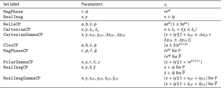
d1d2d3, as in Eq.(24), it is necessary to define the parameterisation of the complex coefficients cjdefined in Eq.(3). Several different parametrisations have been used in the literature and are available inLaura++— a complete list is

given inTable 1. These can be separated into two categories: cases in which it is assumed that there is no difference between the decay of

Pand itsCP-conjugatePand cases in which suchCP-violating differences are accommodated.

In the former case, the signal model is constructed by passing the corresponding

LauIsobarDynamics

instance to a

LauSimpleFit-Model

object, which inherits from the abstract base class

LauAbsFitModel

. The fit model classes implement the functions needed to generate events according to the DP model as well as to perform fits to data. In the latter case, the decays of each ofPandPshould be represented by their own

LauDaughters

instance. These are used to construct two instances of

LauIsobarDynamics

, which in turn are used to construct an instance of the

LauCPFitModel

class that, like

LauSimpleFitModel

, also inherits from

LauAbsFitModel

.

TheFjterms in Eq.(21)are calculated using the amplitudes that make up the

LauIsobarDynamics

model. The complex coefficients

cjare each represented by an object inheriting from the

LauAbsCoeffSet

base class, which provides an abstract interface for combining

a set of real parameters to form the complexcj. Each coefficient is constructed by providing the name of the resonancejand a series

of parameter values that will be used to form the complex numbercj. They are then applied to the model using the

setAmpCoeffSet

function of the

LauSimpleFitModel

or

LauCPFitModel

class. Checks are made to ensure that the coefficient name matches that of one of the components of the isobar model. The coefficient is then assigned to that component. As such the various coefficients are reordered to match the ordering in the

LauIsobarDynamics

model(s).

5. Implementation of efficiency and resolution effects

As discussed in Section3, in an experimental analysis it is usually necessary to modify the signal PDF in order to account for effects such as the variation of the reconstruction and selection efficiency over the DP and detector resolution or misreconstruction. In this section we describe the classes and methods in theLaura++package that are used to implement these modifications to the pure physics PDF described previously.

[image:11.595.122.489.99.244.2]

Table 1

List of coefficient sets to representcjin Eq.(3), separated into cases whereCPconservation is assumed and those where CPviolation is accommodated in the model. Where parameters are preceded by±signs in the expressions forcj, the

+(−) sign corresponds to the usage forP(P) decays. The corresponding class for each set isLauLabelCoeffSet, whereLabelis the set label given below.

Set label Parameters cj

MagPhase r,φ reiφ

RealImag x,y x+iy

BelleCP a,b,δ,φ aeiδ_(1±beiφ₎

CartesianCP x,y,δx,δy x±δx+i(y±δy)

CartesianGammaCP x,y,xCP,yCP,∆xCP,∆yCP (x+iy)[1+xCP±∆xCP+ i(yCP±∆yCP)]

CleoCP a,b,δ,φ (a±b)ei(δ±φ)

MagPhaseCP r,φ,¯r,_φ¯ _reiφ_forP

¯

rei_φ¯

forP

PolarGammaCP x,y,r,δ,γ (x+iy)(1+rei(δ±γ)₎

RealImagCP x,y,x¯,¯y x+iyforP

¯

x+iy¯forP

RealImagGammaCP x,y,xCP,yCP,x¯CP,y¯CP (x+iy)(1+xCP+iyCP) forP

(x+iy)(1+ ¯xCP+iy¯CP) forP

5.1. Efficiency

The variation of the signal efficiency over the DP,

ϵ

(m2

13

,

m223), is implemented by the

LauEffModel

class. Its constructor requires a

LauDaughters

object, which defines the kinematic boundary, as well as a

LauVetoes

object, which is used to specify any region in the DP that has been excluded from the analysis (perhaps to remove particular sources of background or to exclude a region of phase space where the efficiency variation is poorly understood). The signal efficiency is set to zero inside a vetoed region; the resulting discontinuity at the boundary motivates different treatment of vetoes to other sources of inefficiency that vary smoothly across the DP. Vetoes can be added using the

addMassVeto

or

addMassSqVeto

functions of the

LauVetoes

class, which require the bachelor daughter index as well as the lower and upper invariant mass (or mass-squared) values for each exclusion region. Since version

v3r2

ofLaura++, vetoes are automatically symmetrised as appropriate for DPs containing two or three identical particles in the final state.

All other information on the efficiency variation over the DP needs to be supplied in the form of a uniformly binned two-dimensional

Roothistogram. Alternatively, a set of histograms can be provided; in this case the total efficiency is obtained by multiplying the efficiencies at the appropriate position in phase space from each of the components. This provides a convenient way to assess the impact of systematic uncertainties from different contributions to the total efficiency. Each of these component efficiency histograms can have different binning. Efficiency histograms will usually be constructed by applying all selection requirements to a simulated sample of signal decays that has been passed through a full detector simulation. A ratio is then formed of all decays that survive the reconstruction and selection to all those that were originally generated. Since the effect of explicit vetoes in the phase space is separately accounted for, it is advised that these are not applied when constructing the numerator of the efficiency histogram.

As previously mentioned in Section4.1.1, signal events often occupy regions close to the kinematic boundaries. The SDP transformation defined in Eq.(27)can be used to spread out these regions so that the efficiency variation can be modelled more accurately. As such, the

LauEffModel

class will accept histograms that have been created in eitherm2

13–m223orm

′ –

θ

′

space.

The histogram can then be supplied to the

LauEffModel

class via the

setEffHisto

or

setEffSpline

function as appropriate. Where the total efficiency is to be obtained from the product of several components, further histograms can be included with the

addEffHisto

and

addEffSpline

functions. In each case, a boolean argument

squareDP

is used to indicate the space in which the histogram has been defined. For symmetric DPs, there is also the option to specify that the histogram provided has already been folded and hence only occupies the upper half of the full DP (or the corresponding lower half of the SDP). Internally, each histogram is stored as a

Lau2DHistDP

or

Lau2DSplineDP

object, which implement (optional) bilinear or cubic spline interpolation methods, respectively.

Functionality is also available to help estimate systematic uncertainties due to imperfect knowledge of the efficiency variation by creating Gaussian fluctuations in the bin entries. The fluctuations are based on the uncertainties provided by the user, which, depending on the function used to provide the histogram, can be asymmetric. It is up to the user as to whether the provided uncertainties are simply due to the limited size of the simulated sample or whether they also account for effects such as possible disagreements between data and simulation. The fluctuations are activated by providing optional boolean arguments to the function where the histogram is provided.

5.2. Resolution

The self cross-feed component of the signal likelihood, modelled as described in Eq.(25), is implemented using information from the

LauScfMap

class, which stores all possible values of

w

scfvia its

setHistos

function. As for the description of the efficiency, the histograms

used to describe

w

scfandfscfcan be constructed in eitherm213–m 2

23orm

′

–

θ

′space. However, to simplify the implementation inLaura++it is currently required that all histograms related to the description of resolution have the same binning.

The implementation proceeds as follows. Consider a SDP describing the true position,strue, divided into a uniformly binned

two-dimensional histogram. Each bin will have associated with it another two-two-dimensional histogram, with identical binning, whose entries give the migration probability

w

scf(sreco

,

strue) of the true position (given by the original bin centre) being reconstructed in the bin that

containssreco. These can be constructed as follows:

•

Each histogram contains only the events that were generated in a given true bin.

•

The events are plotted at their reconstructed co-ordinates.

Some histograms may be empty if there were no events generated in that bin, although this is of course dependent on the size of the samples used and the size of the bins. The order of the histograms in the vector supplied to the

setHistos

function should be in terms of theRoot‘‘global bin number’’.

The

splitSignalComponent

method of

LauSimpleFitModel

and

LauCPFitModel

takes a

LauScfMap

object as an argument, as well as a two-dimensionalRoothistogram whose entries givefscf(strue). The fit models then use this information to evaluate the self

cross-feed contribution to the likelihood. In the ideal case of Eq.(25)this is described by an integral; in practice this becomes a summation,

∫

fscf(strue)

w

scf(sreco

,

strue)Psig(strue)dstrue

↪

→

∑

i

[

⟨

_ˆ

fscf(

ˆ

strue i)

⟩ ⟨

ˆ

w

scf(

ˆ

sreco

,

s

ˆ

true i)

⟩

Psig(

ˆ

strue i)∆Ω

(

ˆ

strue i)

∆Ω(

ˆ

sreco)

]

,

(31)

where the hat (

ˆ

) notation is used to indicate quantities evaluated in the SDP (as is the case in this example), and the bracket (

⟨ ⟩

) notes quantities obtained from histograms. The pure signal PDFPsigis as in Eq.(24), evaluated at the position corresponding to the SDP point at

the centre of the

ˆ

strue ibin. The phase space factors∆Ωare equal to∆m′∆

θ

′

|

J

|

where the SDP bin size is given by∆m′∆

θ

′and the Jacobian

of the SDP transformation is that of Eq.(28); since equal binning is required, the ratio of phase space factors reduces to a ratio of Jacobians.

6. Implementation of background components

6.1. Dalitz-plot distributions

Backgrounds in the data sample can be taken into account by including them in the total likelihood defined in Eq.(26). This means that the DP distributions of all background categories need to be provided. In an analogous way to the implementation of the signal efficiency described in the previous section, the DP distribution of each background category is represented with a uniformly binned two-dimensional

Roothistogram.

Background contributions are handled inLaura++as follows. Firstly, the names of all background categories need to be provided to

the fit model via the

setBkgndClassNames

function of the appropriate

LauAbsFitModel

class. Then, each named category needs to have its DP distribution defined and added to the fit model. This is achieved by supplying one (or more if the model subdivides the data to account for effects such asCPviolation)

LauBkgndDPModel

object. The constructor of the

LauBkgndDPModel

class requires pointers to the usual

LauDaughters

and

LauVetoes

objects. The histogram is supplied to the

LauBkgndDPModel

object via its

setBkgndHisto

(

setBkgndSpline

) function, and is then internally stored as a

Lau2DHistDPPdf

(

Lau2DSplineDPPdf

) object that implements bilinear (cubic spline) interpolation. The PDF value is then calculated as the interpolated number of background eventsB(m2

13

,

m223) divided by the

total integrated area of the histogram:

P_bkgnd

=

B(m

2 13

,

m223)

∫∫

DP B(m 2 13

,

m

2

23)dm

2

13dm

2 23

.

(32)

Like signal events, backgrounds also tend to populate regions close to the kinematic boundaries of the DP. Therefore, the use of histograms in the SDP space can improve the modelling of backgrounds. This is achieved by providing a histogram in m′

–

θ

′ space and setting the

squareDP

boolean flag to true in the

setBkgndHisto

or

setBkgndSpline

functions of

LauBkgndDPModel

. The normalisation of these PDFs then automatically includes the Jacobian for transforming from normal to square Dalitz-plot space.

Some special treatment is necessary for backgrounds modelled from sources that contain contributions that are vetoed in the DP fit. Following the example of Section3, the combinatorial background toB−

_→

K−

_π

+

_π

−

decays may be modelled from a sideband in theB

candidate mass distribution that also contains some genuineD0

→

K−

π

+decays. The histogram binning will introduce some smearing of such contributions, so that once the veto is applied later some residual background may remain. In principle this can be avoided with sufficiently fine histogram bins, but this will often be impractical due to finite sample sizes. Instead, and in contrast to the procedure for efficiency histograms described in Section5.1, the veto should be applied when the background histogram is made. This will, however, lead to an underestimation of the background that is being modelled (in the example above, of the random combinations of three tracks) within bins that lie partially inside the vetoed regions. To correct for this effect, each background histogram needs to be divided by another histogram (with the same binning) whose entries contain the fraction of events, generated from a high statistics sample that is uniform in phase space, that lie outside any veto region; bins that are completely outside (inside) a veto have a weight of unity (zero), and division by zero is interpreted as zero weight. The histogram supplied to

LauBkgndDPModel

should already have had this correction applied to it.

6.2. Other discriminating variables

When fitting a data sample that contains (significant) backgrounds, additional discriminating variables can be included in the total likelihood function defined in Eq.(26), in order to provide improved separation between signal and background categories. Examples of such discriminating variables include the mass of the parent particlePcandidate and the output of a multivariate discriminant to separate signal from background. Assuming that all of the variables

⃗

x

=

(x1

,

x2

, . . . ,

xn) are uncorrelated, the PDFPkj of the signal

or background categoryk, for eventj, is given by the product of the individual variable PDFs (including that of the DP distribution):

P_kj(

⃗

x)

=

P_kj(x1)

×

Pkj(x2)

× · · · ×

Pkj(xn).

Additional PDFs are represented by classes that inherit from

LauAbsPdf

, whose constructor requires the variable name, a vector of the PDF parameters, as well as minimum and maximum abscissas that specify the variable range. Each class implements the member function for evaluating the PDF function at a given abscissa value and that for evaluating the maximum value of the PDF in the fitted range. A list of classes that can be used for additional PDFs is given inAppendix D. Each PDF needs to be added to the fit model; for

LauSimpleFitModel

(

LauCPFitModel

), signal PDFs are added using the

setSignalPdf

(

setSignalPdfs

) function, self cross-feed PDFs are included via