Frequentist model averaging for
threshold models
Gao, Yan and Zhang, Xinyu and Wang, Shouyang and
Chong, Terence Tai Leung and Zou, Guohua
Minzu University of China, Chinese Academy of Sciences, The
Chinese University of Hong Kong, Capital Normal University
28 November 2017
Online at
https://mpra.ub.uni-muenchen.de/92036/
Frequentist Model Averaging for Threshold Models
Yan Gao1,2, Xinyu Zhang2,3,∗, Shouyang Wang2,
Terence Tai-leung Chong4and Guohua Zou5
1Department of Statistics, College of Science, Minzu University of China, Beijing 100081, China 2Academy of Mathematics and Systems Science, Chinese Academy of Sciences, Beijing 100190, China
3College of Mathematics and Statistics, Qingdao University, Qingdao 266071, China 4 Department of Economics, The Chinese University of Hong Kong, Shatin, Hong Kong
and5School of Mathematical Science, Capital Normal University, Beijing 100037, China
ABSTRACT: This paper develops a frequentist model averaging approach for threshold model spec-ifications. The resulting estimator is proved to be asymptotically optimal in the sense of achieving the
lowest possible squared errors. Especially, when combining estimators from threshold
autoregres-sive models, this approach is also proved to be asymptotically optimal. Simulation results show that for the situation where the existing model averaging approach is not applicable, our proposed model
averaging approach has a good performance; for the other situations, our proposed model averaging approach performs marginally better than other commonly used model selection and model
aver-aging methods. An empirical application of our approach on the US unemployment data is given.
Key words:Asymptotic optimality, Generalized cross-validation, Model averaging, Threshold model.
1. Introduction
Threshold models have developed rapidly over the past three decades since the
pio-neering studies of Tong and Lim (1980) and Tong (1983, 1990). Chan (1993) studied
the consistency and limiting distribution of the estimated parameters of threshold
au-toregressive (TAR) models. Hansen (2000) developed the asymptotic distribution for
the threshold estimator with a shrinking threshold effect. Delgado and Hidalgo (2000)
proposed estimators for the location and size of structural breaks in a nonparametric
re-gression model. An important question in the study of threshold models is the selection
of a candidate model. Kapetanios (2001) compared the small sample performance of
different information criteria in threshold models. Model averaging (MA), as an
alter-native to the model selection (MS), considers model uncertainty by weighting estimators
across different models, instead of relying entirely upon a single model. The MA
timator is generally more stable than the MS estimator, as a small change in data can
lead to a significant change in the selection of the optimal model (Yang 2001; Shen and
Huang 2006).
There are two strands of literature on model averaging: Bayesian model averaging
(BMA) and frequentist model averaging (FMA). Cuaresma and Doppelhofer (2007)
ap-plied the BMA to take an average over possible threshold effects and associated
thresh-old observations. From the frequentist perspective, there are two research fields on
model averaging. One is on the limiting distribution theory of FMA estimator; see, for
example, Hjort and Claeskens (2003) and Xu et al. (2013). The other is on how to
choose weights in model averaging. Hansen (2009) applied Mallows model averaging
(MMA) in weight choice of averaging threshold models. He performed averaging on
models with and without a threshold effect, but did not consider models with different
threshold parameters and explanatory variables.
In the current paper, we explore how the FMA approach can be used to obtain an
average of threshold models. Two cases are considered. In Case I, we first estimate
the threshold parameters of different candidate models, and then perform averaging on
these threshold models with different explanatory variables. In particular, we consider
the averaging of TAR models. In Case II, models with a break at different observed
threshold points are considered as different models. We do not estimate the threshold
values in this case. In MMA, the variance of random errorσ2is estimated by the model
with the largest number of variables (referred to as the largest model), which leads to
the following two problems:
(i) For Case II, the largest model is not unique.
(ii) Even if there exists a unique largest model, using it to estimateσ2 places too much
confidence on a single model.
To address these two problems, this paper develops a new MA approach based
on the approximate generalized cross-validation (GCV) method of Craven and Wahba
(1979), for which the existence of a unique largest model is unnecessary and the
estima-tion ofσ2depends on the weights of MA. The resulting averaging estimator is proved to
be asymptotically optimal in achieving the lowest possible squared error. In Case I, since
the estimator of the threshold parameter is random, the associated coefficient estimator
is not a linear combination of the dependent variable. As a result, the proof of
asymptot-ic optimality is more challenging than the existing proofs for other MA methods, such
as MMA and optimal frequentist model averaging (Liang et al. 2011).
The simulation results show that in most cases the new MA estimators have lower MSEs
than the MS estimators and other MA estimators. We also apply our method to analyse
the unemployment data for the US and show that our model averaging estimator has
better forecasting performance than its competitors.
The remainder of this paper is organized as follows. Section 2 introduces the
threshold model and the estimation method. Section 3 provides the criterion for
select-ing weights and develops the asymptotic optimality theory of the averagselect-ing estimator.
Section 4 compares our MA estimators with some commonly used MS and MA
estima-tors. Section 5 presents an empirical application of our method. Section 6 concludes the
paper. The technical proofs are relegated to the Appendix.
2. The Model
We consider a threshold regression model with a possible threshold effect,
yi=µi+ei =x′iβ1I(zi ≤γ) +x′iβ2I(zi > γ) +ei, i= 1, . . . , n, (1)
where yi is the dependent variable, xi = (xi1, xi2, . . .) are the explanatory variables
which can be countably infinite, β1 and β2 are two vectors of coefficients, I(·) is an
indicator function,ziis the threshold variable and can be be part ofxi,γis the
thresh-old parameter, and ei’s are errors withE(ei|xi) = 0 andE(e2i|xi) = σ2. Let Y =
(y1, . . . , yn)′,e = (e1, . . . , en)′ andµ = (µ1, . . . , µn)′. In application,µis generally
approximated by
µ≈X(γ)β,
whereX(γ)is ann×2ηmatrix with theith row((xi1, . . . , xiη)I(zi ≤γ),(xi1, . . . , xiη)
I(zi > γ))andβis the corresponding coefficient vector. Since the threshold models can
be regarded as piecewise linear models, the estimation and averaging methods for linear
models can be employed. In a similar way to Hansen (2000), we estimate the parameters
by conditional least squares. Let
S(β, γ) = (Y −X(γ)β)′(Y −X(γ)β), (2)
which is the sum of squared errors (SSE). By minimizing (2), we obtain all the
estima-tors. We assume thatγ belongs to a bounded setΓ = [γ,γ¯]. First, givenγ,βˆ(γ)can
be obtained by minimizingS(β, γ). We then replaceβ byβˆ(γ), and the SSE becomes
S( ˆβ(γ), γ), witch is written asS(γ). The estimate ofγ is defined as:
ˆ
γ =arg min
γ∈Γn
whereΓn={z1, . . . , zn} ∩Γ. Letz(i)be theith smallest element in{z1, . . . , zn}. To
ensure that the model is estimable,Γis assumed to satisfyγ ≥z(η+1)and¯γ ≤z(n−η−1).
We also assume thatΓnis non-empty.
3. Model Averaging and Weight Choice
In this section, we propose a new criterion for selecting the optimal weights. Two cases
are considered. For Case I, we consider the uncertainty caused only by different
ex-planatory variables, and in Case II, we perform averaging on both different threshold
parameters and different explanatory variables. All limiting processes discussed in this
section are with respect ton→ ∞.
3.1. Averaging for Models with Estimatedγ
In this subsection, we aim to average threshold models with different explanatory
vari-ables. We consider model averaging for threshold models that do not contain lagged
dependent variables, and model averaging for TAR models. Moreover, we show the
asymptotic optimality of the proposed MA estimators in both cases under certain
regu-larity conditions.
3.1.1. Averaging for threshold models without lagged dependent variables
Assume that the errors(e1, . . . , en)are i.i.d.. We consider a sequence of approximating
models among which themth model includeskm explanatory variables that form the
vectorx(m)i. Specifically, themth model is:
Y =X(m)(γ)β(m)+e(m), (3)
whereX(m)(γ)is a matrix stacking the vectors(x′
(m)iI(zi ≤γ), x′(m)iI(zi> γ))and of
full column rank,β(m)is the coefficient vector ofX(m)(γ), e(m) = µC(m)(γ) +e, and
the termµC(m)(γ) =µ−X(m)(γ)β(m)of which is the approximation error of model (3).
Following the estimation method in Section 2, we can obtain the estimated
thresh-old parameterγˆ(m)and coefficient
ˆ
β(m)= (X(′m)(ˆγ(m))X(m)(ˆγ(m)))−1X(′m)(ˆγ(m))Y (4)
under themth model. LetXˆ(m) =X(m)(ˆγ(m))andPˆ(m) = ˆX(m)( ˆX(′m)Xˆ(m))−1Xˆ(′m),
so that the estimator ofµunder themth candidate model is given byµˆ(m) = ˆP(m)Y.
Denotew= (w1, . . . , wM)′, a weight vector in the unit simplex inRM
Hn= n
w∈[0,1]M : M X
m=1
wm = 1 o
whereM is the number of candidate models. Note thatHn is a continuous set and is
different from the weight set in Hansen (2007), which is discrete. In addition, Cheng et
al. (2015) used a continues weight set, which is more general than the discrete set of
Hansen (2007) but is still a subset ofHn. The MA estimator ofµcan be expressed as
ˆ
µ(w) = M X
m=1
wmµˆ(m)=
M X
m=1
wmPˆ(m)Y ≡Pˆ(w)Y,
where Pˆ(w) = PMm=1wmPˆ(m) is symmetric but not necessarily idempotent. The
squared error is Ln(w) = kµˆ(w) − µk2, and the corresponding risk is Rn(w) =
E(Ln(w)|X, Z), whereX = (x1, . . . , xn)′andZ= (z1, . . . , zn)′.
Whenσ2is known, one may obtain weights by minimizing the following Mallows’
criterion proposed by Hansen (2007):
Cn(w) =kY −µˆ(w)k2+ 2σ2trPˆ(w).
Sinceσ2 is usually unknown in practice, Hansen (2007) suggested estimating it by the
largest candidate model, i.e.,
ˆ
σ2= (n−kM∗)−1kY −µˆM∗k2,
whereM∗ = arg maxm∈{1,...,M}km. It is shown that as n → ∞, ifkM∗ → ∞and
kM∗/n → 0, thenσˆ2 is consistent and the asymptotic optimality result still holds for
unknownσ2.
In time series case, Hansen (2008) applied this criterion to averaging autoregressive
models. However, the largest model may not be unique in practice. In fact, even if the
largest model is unique, using the single model to estimate σ2 may deviate, in some
sense, from the objective of model averaging. Motivated by these concerns, we develop
a new least squares MA estimator for threshold models. The criterion for selecting
weights is as follows:
Ln(w) =kY −µˆ(w)k2
1 + 2trPˆ(w)
n
. (5)
If we set one component of the weight vectorwto be 1 and the others to be 0, then (5)
reduces to a criterion for model selection. Therefore, one may approximate the GCV
criterion by the MS version of (5) and use it to relate GCV to Mallows’Cp (Li 1987).
For any fixed w in (5), kY −µˆ(w)k2/n is the mean of residual squared sums of the
MA estimatorµˆ(w). If we take it as an estimator ofσ2, thenL
n(w)can be regarded as
σ2 based on the largest model. We use a averaging estimator ofσ2 instead. Thus, our criterion can be viewed as an adjusted Mallows criterion, which can be used in more
general cases because MMA would be infeasible when the largest model is not unique,
as is the case in Subsection 4.2. If the covariance matrix of the error term e is not
diagonal, to estimate the inverse of the covariance matrix, we may use the estimators
proposed by Cheng et al. (2014) and Cheng et al. (2015).
We rewriteLn(w)asLn(w) = w′eˆ′ˆew(1 + 2w′K/n)for simplicity, whereK =
(k1, ..., kM)′,ˆe= (ˆe(1), . . . ,ˆe(M))andˆe(m) =Y −µˆ(m). When constrainingwtoHn,
we can obtain weights through minimizingLn(w), i.e.,wˆ= arg minw∈HnLn(w). The
estimatorµˆ( ˆw)is referred to as the Adjusted Mallows Model Averaging (AMMA)
esti-mator ofµhereafter. Note that althoughLn(w)is a cubic function ofw, the numerical
algorithms for minimizing such a criterion are actually readily available. For example,
one can use ’solnp’ in the R package ’Rsolnp’. Therefore, our AMMA approach can be
easily performed in practice.
Note that for each candidate model, the estimator ofµdepends on a random item
ˆ
γm, thus causing problems for conducting the asymptotic optimality. So the theory in
this subsection is not just a extension of that of Hansen (2007). To solve this problem,
we try to find a properly defined limit forγˆ(m)under each candidate model. We assume
that there exists a constantγ∗
(m)such thatγˆ(m)
p −→γ∗
(m), whereγ(∗m)is not necessarily
equal to the true valueγ0. Ifzi =i/nandkm is bounded, the convergency was proved
by Koo and Seo (2015). However, ifkmis related withn, it requires future work.
LetX(∗m) =X(m)(γ(∗m)),P(∗m) =X(∗m) X(∗′m)X(∗m)
−1
X(∗′m),P∗(w) =PMm=1wm
P(∗m),A∗(w) =In−P∗(w), andLn∗(w) =kP∗(w)Y −µk2. Then we haveR∗n(w)≡
E(L∗n(w)|X, Z) = kA∗(w)µk2 + σ2trP∗2(w). Define ξn∗ = infw∈HnR∗n(w) and
λmax(A) as the maximum singular value of matrixA. The following theorem states
the asymptotic optimality of the AMMA estimator.
THEOREM1. For some finite integerG≥1, if
E(e4iG|xi)<∞, (6)
M ξn∗−2G
M X
m=1
R∗n(w0m)G−→p 0, (7)
nξn∗−1 max
1≤m≤Mλmax(P
∗
(m)−Pˆ(m))
p
−→0, (8)
and
kµk2 =Op(n), (10)
then
Ln( ˆw) infw∈HnLn(w)
p
−→1, (11)
wherea1is a constant, andwm0 is anM×1vector in which themth element is one and the others are zeros.
Proof: See the Appendix.
Condition (6) is a moment condition and requires the regression error distribution
to have sufficiently thin tails. For example, it excludes the Cauchy distribution and
holds for Gaussian distribution. Condition (9) requires that the numbers of covariates
in candidate models do not increase faster thann1/2. Condition (10) is on the sum of
µ21, . . . , µ2n and need only thatµ21, . . . , µ2n do not expand with n. Condition (7) is a commonly used condition in the model averaging literature such as Wan et al. (2010)
and Liu and Okui (2013). To explain this condition, we consider a situation withξ∗
n =
na, sup
w∈HnR∗n(w) = n
b, and 0 < a ≤ b < 1, then Condition (7) is implied by
M2nG(b−2a)→0, which holds whenb <2aandM doest not increase withntoo fast.
Cheng et al. (2015) pointed out that Condition (7) will preclude some good models with
smallerLn(w)in linear cases. Similarly, it still may happen in the threshold models.
However, they select weights on a narrower set compared with our continuous setHn.
Thus, we need to add Condition (7) to ensure the asymptotic optimality of AMMA,
which meansM can not increase withnas fast as it in Cheng et al. (2015). Condition
(8) puts some restrictions on the order ofξn and the convergence rate of the elements
of matrix Pˆ(m) −P∗
(m). Note that because ˆγ(m)
p −→ γ∗
(m), the elements of matrix
ˆ
P(m)−Pˆ∗
(m)converge to zeros. The proof of (58) in the Appendix shows that Condition
(8) can be satisfied whenkM∗is bounded.
3.1.2. Averaging for TAR Models
The TAR model is a special case among threshold models and is widely used in
empir-ical analysis. However, when averaging TAR models, the asymptotic theory developed
above is no longer valid due to serial dependence and the existence of lagged
models1. In the same way as in Subsection 3.1.1, we have
yi = µi+ei
= (β10+
p1
X
j=1
β1jyi−j)I(zi ≤γ) + (β20+
p2
X
j=1
β2jyi−j)I(zi > γ)
+ei, i= 1, . . . , n,
wherepk is the lag order for regimek(k = 1,2),ei’s are white noise with mean zero
and variance σ2 and β
kj’s are autoregressive coefficients with Ppkj=1|βkj| < 1 (k =
1,2). For simplicity, we set p1 = p2 = p, where p can be infinite. In this case,
xi = (1, yi−1, . . . , yi−p)′ and each regime is an AR(km) process in the mth model.
We assume that for eachm,kmis fixed, soM is bounded.
We focus onµand apply the AMMA method to select the weights. LetQ∗n(w) =
kA∗(w)µk2+σ2tr(P∗2(w))andζn∗ = infw∈HnQ∗n(w). To study the asymptotic
opti-mality of the MA estimator, we make the following assumptions:
(a.1){xi, zi, ei}is strictly stationary and ergodic, andE(ei|σ(xi, xi−1, . . .)) = 0, where
σ(xi, xi−1, . . .)is theσ-algebra generated byxi, xi−1, . . ..
(a.2)E|yi|4<∞andE|yiei|4<∞.
(a.3) Letf2(z|γˆ(m))be the conditional density ofzi givenˆγ(m). Uniformly forz ∈ Γ
andγˆ(m)∈Γ, the conditional densityf2(z|ˆγ(m))is bounded by a finite constantf¯2, and
the conditional expectationE(|xijxik||zi =γ,γˆ(m))withziandγˆ(m)given is bounded.
(a.4)E|γˆ(m)−γ∗
(m)|=O(n−ρ)for some constant0< ρ≤1, m= 1, . . . , M.
Assumptions (a.1) and (a.2) are common assumptions for stationary processes. In
real data analysis, if the series is non-stationary, we can use some data conversion
meth-ods, such as the differential operator and seasonal adjustment to get a stationary series.
Assumption (a.3) requires the conditional density and expectation are bounded.
As-sumption (a.4) is based on the result of Koo and Seo (2015), who showed that the
con-vergence rate ofγˆcan be as fast asT−1/3 for the structural break model. Under these
assumptions we have the following theorem.
THEOREM2. If Assumptions (a.1)∼(a.4) and Condition (10) are satisfied and
n1−ρ/2ζn∗−1−→p 0, (12)
then (11) is valid.
1Although Hansen (2008, 2009) studied averaging estimators in time series models, they did not develop the
Proof: See the Appendix.
3.2. Averaging for Models without Estimatingγ
In this subsection, we average models with different threshold parameters and different
explanatory variables simultaneously using the models set up in Subsection 3.1.1. Let
|Γn|be the size ofΓn. Since there are|Γn|possible threshold points, there will be|Γn|
models with the same explanatory variables. Letγ(s) be thesth item of Γn. Assume
that themsth candidate model contains km explanatory variables, withγ(s) being the
threshold parameter. Then the threshold parameter in every candidate model can be
regarded as a fixed constant. Therefore, the coefficient estimated by themsth model is:
e
β(ms)= (X(′m)(γ(s))X(m)(γ(s)))−1X(′m)(γ(s))Y,
and the estimator ofµis given by
e
µ(ms)=X(m)(γ(s))(X(′m)(γ(s))X(m)(γ(s)))−1X(′m)(γ(s))Y ≡P(m)(γ(s))Y.
Letw = (w11, . . . , wM|Γn|)′ andHen =
n
w ∈ [0,1]M|Γn| :PM m=1
P|Γn|
s=1wms = 1 o
,
which is also a continuous weight set, so that the averaging estimator ofµis:
e µ(w) =
M X
m=1 |Γn| X
s=1
wmseµ(ms)=
M X
m=1 |Γn| X
s=1
wmsP(m)(γ(s))Y ≡P(w)Y.
The squared error isLen(w) = kµe(w)−µk2, and the corresponding risk isRen(w) =
E(Len(w)|X, Z). Letξen= infw∈HenRen(w). In this subsection, the largest model is not
unique, so the Mallows’ criterion does not apply. In light of this concern, we make use
of the AMMA idea, that is, we select weights by the following criterion:
e
Ln(w) =kY −µe(w)k21 + 2trP(w)
n
.
Letwe = arg minw
∈HenLen(w)and the corresponding AMMA estimator be eµ(we). The
following theorem guarantees the asymptotic optimality of the AMMA estimator.
THEOREM3. For some finite integerG≥1, if Conditions (6), (9) and
M|Γn|ξen−2G M X
m=1 |Γn| X
s=1
e
Rn(w0ms) G p
−→0, (13)
hold, then
e Ln(we) infw∈He
nLen(w) p
In the current case, since the threshold parameter is known in every candidate
mod-el, the proof of Theorem 3 is more straightforward than that of Theorem 1. We only
provide a simple explanation in the Appendix. The detailed proof is available on request
from the authors. Note that Condition (13) is similar to Condition (7).
4. Simulations
In this section, we conduct three simulation studies to compare the performance of the
MA estimator and the MS estimator. The first simulation performs averaging for
mod-els with different explanatory variables and i.i.d errors, the second simulation performs
averaging for models with different explanatory variables and threshold parameters, and
the third simulation performs averaging for TAR models with different orders.
4.1. Simulation I: Averaging for Models with Estimatedγ
The data generating process is:
yi=µi+ei =
∞
X
j=1
xijβ1jI(xi3 ≤γ) + ∞
X
j=1
xijβ2jI(xi3 > γ) +ei, i= 1, . . . , n,
whereγ = 0,xi1 = 1, all otherxij’s andei’s come fromN(0,1)and are independent
of one another, and the coefficients β11 = c, the remaining β1j = cj−ζ with ζ =
0.25,0.5,0.75controlling the decay rate of the coefficients, andβ2=aβ1 witha= 1.5
andc >0. The difference between coefficients is denoted bya. The parametercis set
to make the populationR2 =var(yi−ei)/var(yi)vary on a grid from 0.1 to 0.9. To
let the threshold variablexi3 appear in each candidate model, we set themth candidate
model to include the firstm+2explanatory variables (m= 1, . . . , M), andM = 3n1/3.
When estimatingγ, we restrict it to the set containing the20%,25%, . . . ,80%quantiles
of{xi3}for decreasing computation time, as suggested by Hansen (2000). The sample
size is set at 60, 100, 250 and 400. To evaluate the performance of the estimators, we
simulate 500 replications and compute mean squared risk by
1 500
500
X
r=1
n X
i=1
(ˆµ(ir)−µi)2, (15)
whereµˆ(ir) is the estimates ofµ in therth replication. For each parameterization, we
normalize the risks by dividing the risk by the infeasible optimal risk (the risk of the
best single model).
We compare our averaging estimator with the AIC and BIC model selection
where σˆm2 = kY − µˆ(m)k2/n, and the BIC score for the mth model is BICm =
nlog ˆσ2m+kmlogn. We also compare our averaging estimator with the existing model
averaging methods: MMA, Smoothed AIC (S-AIC), and Smoothed BIC (S-BIC),
pro-posed in Buckland et al. (1997) and ARM (Adaptive Regression by Mixing), an
adap-tive method developed by Yang (2001). The S-AIC method assigns weightwAIC,m =
exp(−AICm/2)/PMm=1exp(−AICm/2)to themth model and the S-BIC method
as-signs weight wBIC,m = exp(−BICm/2)/PMs=1exp(−BICm/2) to the mth model.
The ARM method divides samples into a training part and a testing part. The
parame-ters are estimated by the training samples while the weights are obtained by the testing
samples. For more details, one can refer to Yang (2001).
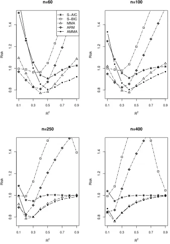
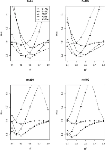
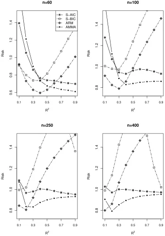
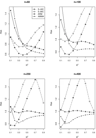
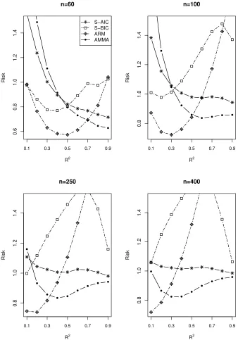
The simulation results are displayed in Figs 1 - 3. In each panel, the relative risk is
displayed on theyaxis and the populationR2is displayed on thexaxis. Since the MA
methods are always better than the MS methods, we only show the MA results to
distin-guish different lines clearly. In addition, we cut off part of the figures to make it easier
to compare AMMA and MMA in some cases. Although some risks do not appear in the
figures, they are all bounded actually. The factors that affect the relative performances
of the competitors includen (sample size), ζ ( the decay rate of the coefficient) and
R2 (population). First, in the majority of cases of{n, ζ, R2}, the AMMA outperforms
S-AIC and S-BIC. Second, the AMMA performs better than the MMA and ARM when
R2 is large; while whenR2 is small, the AMMA performs worse than the MMA and
ARM. Third, whennorζ decreases, the region ofR2 where the AMMA outperforms
the MMA and ARM becomes wider. Fourth, whennincreases, the AMMA and MMA
perform more closely. In addition, we also conduct simulations fora= 0.2anda= 3.
The corresponding results are qualitatively similar to those obtained fora= 1.5.
4.2. Simulation II: Averaging for Models without estimatingγ
The setup of this simulation is the same as that in Subsection 4.1. However, in this
sub-section, we do not estimate the threshold parameter. We average or select among models
with different explanatory variables at all possible threshold points, and do not compare
the AMMA method with the MMA method as MMA is infeasible in this example.
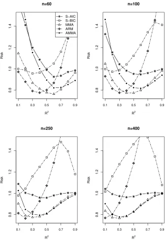
The simulation results are displayed in Figs 4-6. Again, we can find the AMMA
outperforms S-AIC, S-BIC and ARM. The detailed comparison findings are very similar
to those in Simulation I.
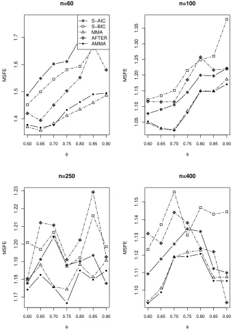
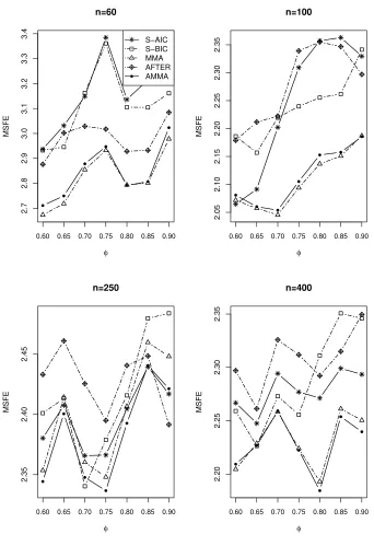
We now investigate the performance of the averaging estimator for TAR models. The
data generating process is as follows:
yi = (β10+
p X
j=1
β1jyi−j)I(yi−d≤γ)+(β20+
p X
j=1
β2jyi−j)I(yi−d> γ)+ei, i= 1, . . . , n,
whereyi−dis the threshold variable anddis the lag order. We seteito be i.i.d. N(0, σ2),
d = 3, γ = 0, p = 6, β10 = 0.5, and β20 = −0.5. The coefficients are generated
by the rule βkj =
5(1 +j)αk(−φ)j
6Ppi=1(1 +i)αkφi, where φ andαk are constants and k = 1,2,
j = 1, . . . , p, which is similar to the setting in Hansen (2008). AsPpj=1|βkj| < 1,
{yn}is stationary. Note thatβki/βkj = 1+1+jiαk(−φ)i−j (i > j), so the item(−φ)i−j
determines the convergence rate of the coefficients. We let α1 = 0.1,α2 = 0.3, n ∈
{60,100,250,400},σ2 = 0.5,1,2andφvary on a grid from 0.6 to 0.9.
Candidate models differ in their lag orders. Identical orders are used in the two
regimes and the threshold parameter is estimated, so we haveM = p = 6candidate
models. Unlike the previous simulations, we also need to estimatedhere. Denote by
ˆ
dm the estimator ofdunder themth candidate model. According to themth candidate
model, the one-step-ahead out-of-sample forecast ofyn+1 givenyn, yn−1, . . .is:
ˆ
yn+1(m) =( ˆβ(m)10+
m X
j=1
ˆ
β(m)1jyn+1−j)I(yn+1−dmˆ ≤γˆ(m))
+ ( ˆβ(m)20+
m X
j=1
ˆ
β(m)2jyn+1−j)I(yn+1−dmˆ >γˆ(m)),
whereβˆ(m)rj is the estimator of β(m)rj forr = 1,2andj = 0, . . . , p. The combined
forecast is given byyˆn+1(w) = PMm=1wmyˆn+1(m). To compare the performance of
model selection and averaging methods, we use 500 replications. For each replication,
we generate a series of sizen+ 1and use the firstnsamples to get the averaged
coeffi-cients. Then we calculate the one-step-ahead out-of-sample prediction and get the mean
squared forecast error (MSFE) given by
1 500
500
X
r=1
(y(nr+1) −yˆn(r+1) )2, (16)
whererdenotes therth replication.
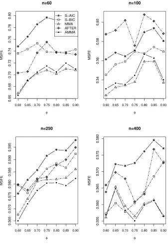
Figs 7-9 show the simulation results. As the ARM method can not be used for
time series prediction, we choose another adaptive method, named AFTER (Aggregated
MMA and AMMA always perform better than the other methods. The factors that
affect the relative performances of the competitors includen (sample size), σ2 (noise
level) andφ (the convergence rate of the coefficients). First, in the majority of cases
of{n, σ2, φ}, the AMMA and MMA outperform S-AIC, S-BIC and AFTER. Second,
whenn= 60,100, the MMA performs better than AMMA in most of values ofφ, while
whenn= 250,400, the AMMA performs better than the MMA in most of values ofφ.
Third, for differentσ2, the comparison results are very similar.
5. Empirical Application
In this section, we apply the averaging approach to a monthly data set for US
unemploy-ment from January 1970 to Dec 2012. The sample size is 516 in total. The unit root test
for threshold model (Caner and Hansen 2001) suggests that the process is a stationary
nonlinear threshold autoregression. The model selection and averaging methods are the
same as those in Simulation III, with the largest order set to be 12. The candidate set
fordis{1,2, . . . ,12}. We use{y1, . . . , yn}to fit the model and predictyn+1. Then,
we use{y2, . . . , yn+1}to fit the model and predictyn+2. By pushing on this procedure
step by step, we can get516−npredictions at last. nis set at 60, 150, 250, and 400.
We compare the AMMA method with the AIC, BIC, S-AIC, S-BIC, AFTER and MMA
methods using the MSFE. We also report the standard deviation (SD) of the squared
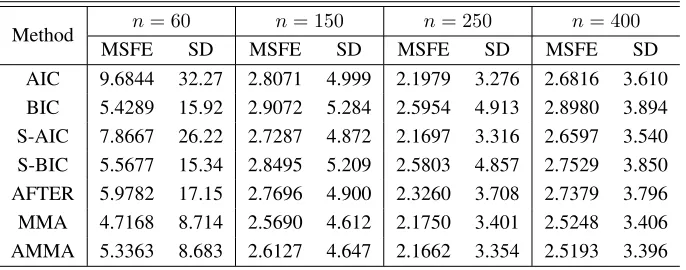
forecast error. The results are shown in Table 1.
The performance of the AMMA estimation is always better than that of the AIC,
BIC, S-AIC and S-BIC methods, since its means are lowest. Whenn = 250andn=
400, the AMMA estimator has lower means than the MMA estimator, while the MMA
[image:14.612.105.448.556.691.2]performs better whenn= 60andn= 150.
Table 1: Squared Forecast Errors of Different Methods (×10−2)
Method n= 60 n= 150 n= 250 n= 400
MSFE SD MSFE SD MSFE SD MSFE SD
6. Conclusion
Threshold models have wide empirical applications. In this paper, two cases of
averag-ing are considered: Case I studies models with different explanatory variables and a
giv-en estimated threshold parameter and Case II studies models with differgiv-ent explanatory
variables at all possible threshold parameters. A new least squares MA estimator–the
AMMA estimator–based on an approximation of GCV is developed. Compared with
the MMA, our AMMA method has wider application because it does not require a
u-nique largest model. When the threshold is estimated, the coefficient estimator in each
candidate model is not a linear combination of the dependent variableY, and the proof
of asymptotic optimality is challenging. Both the simulations and the empirical analysis
show the superiority of the AMMA estimator over some commonly used MS and MA
estimators.
For future research along this line, one could extend our method to allow for
mul-tiple thresholds. For the case of TAR model averaging, one could allow the largest lag
order of the TAR model to be unbounded asymptotically. As this paper mainly focuses
on the asymptotic optimality of the AMMA estimator, the derivation of the consistency
and asymptotic distribution of the AMMA estimator would also be an interesting
fu-ture research topic. Hansen and Racine (2012) developed a jackknife model averaging
(JMA) estimator under heteroscedastic error settings, and Zhang et al. (2013) studied
the JMA in models with dependent data. Therefore, the development of a model
av-eraging method for threshold models with heteroscedastic errors also warrants future
research. Lastly, although we have developed theoretical properties for our model
av-eraging method, they only hold in large sample sense. Understanding the asymptotic
results when the sample size is limited and developing finite sample properties are also
very necessary in the future research.
AcknowledgmentsWe thank the editor and the two anonymous referees for their
con-structive comments. Zhang’s work was partially supported by the National Natural
Sci-ence Foundation of China (Grant nos. 71522004, 11471324, 71463012 and 71631008)
and a grant from the Ministry of Education of China (Grant no. 17YJC910011). Zou’s
work was partially supported by the National Natural Science Foundation of China
(Grant nos. 11529101 and 11331011) and a grant from the Ministry of Science and
Technology of China (Grant no. 2016YFB0502301).
Lemma 1. Let W be a weight vector set which can be related to the sample size n.
Define
w∗=argmin w∈W
(Ln(w) +an(w)). (17)
If
sup w∈W
|an(w)|
Rn(w) p
−→0, (18)
sup w∈W
Ln(w)
Rn(w) − 1 p
−→0, (19)
and there exists a constantκ3such that
inf
w∈WRn(w)≥κ3>0, (20)
then
Ln(w∗) infw∈WLn(w)
p
−→1. (21)
Proof. From the definition of the infimum, there exist a non-negative seriesϑn and a
vectorw(n)∈ Wsuch thatϑn→0and
inf
w∈WLn(w) =Ln(w(n))−ϑn. (22)
In addition, it follows from (19) that
inf w∈W
Ln(w)
Rn(w)
= inf w∈W
Ln(w)
Rn(w) − 1
+ 1
≥ − sup w∈W
Ln(w)
Rn(w) − 1 + 1 p
−→1. (23)
From (20), (23) andϑn→0, we have
inf w∈W
|Ln(w)−ϑn|
Rn(w) ≥
inf w∈W
Ln(w)−ϑn
Rn(w) ≥ inf w∈W
Ln(w)
Rn(w) −
ϑn infw∈WRn(w)
≥ − sup w∈W
Ln(w)
Rn(w)− 1
+ 1−
ϑn infw∈WRn(w) p
−→ 1. (24)
δ >0,
Prinfw∈WLn(w)
Ln(w∗) −1
> δ = Pr
Ln(w∗)−infw∈WLn(w)
Ln(w∗) > δ
= Pr
infw∈W(Ln(w) +an(w))−an(w∗)−infw∈WLn(w)
Ln(w∗)
> δ
≤ Pr
Ln(w(n)) +an(w(n))−an(w∗)−Ln(w(n)) +ϑn
Ln(w∗)
> δ
≤ Pr
|an(w(n))|
Ln(w∗)
+|an(w∗)|
Ln(w∗)
+ ϑn
Ln(w∗)
> δ
≤ Pr
|an(w(n))| infw∈WLn(w) +
|an(w∗)|
Ln(w∗) +
ϑn
Ln(w∗) > δ
= Pr
|an(w(n))|
Ln(w(n))−ϑn
+|an(w∗)|
Ln(w∗)
+ ϑn
Ln(w∗)
> δ ≤ Pr sup w∈W
|an(w)|
Ln(w)−ϑn + sup
w∈W
|an(w)|
Ln(w)
+ sup w∈W
ϑn
Ln(w)
> δ ≤ Pr sup w∈W
|an(w)|
Rn(w) sup w∈W
Rn(w) |Ln(w)−ϑn|
+ sup w∈W
|an(w)|
Rn(w) sup w∈W
Rn(w)
Ln(w)
+ sup w∈W
ϑn
Rn(w) sup w∈W
Rn(w)
Ln(w)
> δ = Pr ( sup w∈W
|an(w)|
Rn(w)
inf w∈W
|Ln(w)−ϑn|
Rn(w) −1
+ sup w∈W
|an(w)|
Rn(w)
inf w∈W
Ln(w)
Rn(w) −1
+ ϑn infw∈WRn(w)
inf w∈W
Ln(w)
Rn(w) −1
> δ )
→ 0. (25)
Therefore,infw∈WLn(w)/Ln(w∗)
p
−→1, which implies (21).
Proof of Theorem 1. First, from the fact thatX(m)(γ)is of full column rank, we have
trPˆ(w) =trP∗(w)≤2PMm=1wmkm. LetAˆ(w) =In−Pˆ(w), so that
Ln(w) =kY −µˆ(w)k2
1 + 2trPˆ(w)
n
=Ln(w) +kek2+ 2µ′( ˆA(w)−A∗(w))e+ 2µ′A∗(w)e
+ 2 σ2trP∗(w)−e′P∗(w)e+ 2e′ P∗(w)−Pˆ(w)e
+ 2trP∗(w) kA∗(w)Yk2/n−σ2
+ 2trP∗(w) kAˆ(w)Yk2− kA∗(w)Yk2/n.
Sincekek2 is unrelated towand Condition (20) withW =H
(7), according to Lemma1, Theorem 1 is valid if
sup w∈Hn
|µ′A∗(w)e|/R∗n(w)−→p 0, (26)
sup w∈Hn
|e′P∗(w)e−σ2trP∗(w)|/R∗n(w)−→p 0, (27)
sup w∈Hn
|L∗n(w)/R∗n(w)−1|−→p 0, (28)
sup w∈Hn
|trP∗(w)(kA∗(w)Yk2/n−σ2)|/R∗n(w)−→p 0, (29)
sup w∈Hn
µ′ P∗(w)−Pˆ(w)e/R∗n(w)−→p 0, (30)
sup w∈Hn
e′ P∗(w)−Pˆ(w)e/R∗n(w)−→p 0, (31)
sup w∈Hn
|Ln(w)−L∗n(w)|/R∗n(w)−→p 0, (32)
and
sup w∈Hn
trP∗(w) kA∗(w)Yk2− kAˆ(w)Yk2/nRn∗(w)−→p 0. (33)
(26)∼(28) can been shown by following the proof of Theorem 1′of Wan et al. (2010).
Therefore, we only need to verify (29)∼(33). First, we prove (29). Note that
sup w∈Hn
|trP∗(w) kA∗(w)Yk2/n−σ2|/R∗n(w)
= sup w∈Hn
ntrP∗(w)
nR∗n(w)
kµ−P∗(w)Yk2+kek2+ 2µ′A∗(w)e−2e′P∗(w)e−nσ2o
≤ sup w∈Hn
L∗n(w)
R∗n(w)wsup∈H
n
trP∗(w)
n + supw∈Hn
2|µ′A∗(w)e| R∗n(w) wsup∈H
n
trP∗(w)
n
+|kek
2−nσ2|
√
n wsup∈Hn 1
R∗
n(w) sup w∈Hn
trP∗(w) √
n
+ sup w∈Hn
2|e′P∗(w)e−σ2trP∗(w)|
R∗
n(w)
sup w∈Hn
trP∗(w)
n
+ 2σ2 sup w∈Hn
1
R∗
n(w) sup w∈Hn
tr2P∗(w)
n .
By the central limit theorem, we have|kek2−nσ2|/√n = Op(1). In addition, it
fol-lows from (7) and (9) that
sup w∈Hn
1
R∗
n(w)
=op(1), sup w∈Hn
tr2P∗(w)/n=O(1) and sup w∈Hn
trP∗(w)/n=o(1).
To prove (30), we observe that
sup w∈Hn
µ′ P∗(w)−Pˆ(w)e/Rn∗(w)
≤ ξ1∗ n
sup w∈Hn
kµk2e′ P∗(w)−Pˆ(w)2e1/2
≤ ξ1∗ n
kµk
√nk√enk n max
1≤m≤Mλmax(P
∗
(m)−Pˆ(m)).
By Conditions (8) and (10), (30) is verified.
Note that
Ln(w) =kek2+kAˆ(w)µk2+kAˆ(w)ek2−2e′Aˆ(w)µ−2e′Aˆ(w)e+ 2µ′Aˆ2(w)e,
so
sup w∈Hn
|Ln(w)−L∗n(w)|/R∗n(w) p −→0⇔
sup w∈Hn
2µ′ P∗(w)−Pˆ(w)µ+ 2µ′ P∗(w)−Pˆ(w)e
−µ′ P∗(w) + ˆP(w) P∗(w)−Pˆ(w)µ
−e′ P∗(w) + ˆP(w) P∗(w)−Pˆ(w)e
−2µ′P∗(w) P∗(w)−Pˆ(w)e−2µ′ P∗(w)−Pˆ(w)Pˆ(w)e/R∗n(w)−→p 0.
Thus, if
sup w∈Hn
µ′ P∗(w) + ˆP(w) P∗(w)−Pˆ(w)µ/Rn∗(w)−→p 0, (34)
sup w∈Hn
e′ P∗(w) + ˆP(w) P∗(w)−Pˆ(w)e/Rn∗(w)−→p 0, (35)
sup w∈Hn
µ′P∗(w) P∗(w)−Pˆ(w)e/R∗n(w)−→p 0, (36)
sup w∈Hn
µ′ P∗(w)−Pˆ(w)Pˆ(w)e/R∗n(w)−→p 0, (37)
and
sup w∈Hn
then (32) is valid. From Condition (8) and the following result
sup w∈Hn
e′ P∗(w) + ˆP(w) P∗(w)−Pˆ(w)e/R∗n(w)
≤ 1
2ξ∗
n sup w∈Hn
e′ P∗(w) + ˆP(w) P∗(w)−Pˆ(w)
+ P∗(w)−Pˆ(w) P∗(w) + ˆP(w)e
≤ kek
2
2ξ∗
n sup w∈Hn
λmax P∗(w) + ˆP(w) P∗(w)−Pˆ(w)
+ P∗(w)−Pˆ(w) P∗(w) + ˆP(w)
≤ kek
2 ξ∗
n sup w∈Hn
λmax P∗(w) + ˆP(w)λmax P∗(w)−Pˆ(w)
≤ kek
2 ξ∗
n sup w∈Hn
λmax P∗(w)
+λmax Pˆ(w)
XM
m=1
wmλmax(P(∗m)−Pˆ(m))
≤ ξ2∗ n
kek2
n n1≤maxm≤Mλmax(P
∗
(m)−Pˆ(m)),
we obtain (35). Similarly, (31), (34) and (38) can be verified. On the other hand,
analo-gous to the proof of (30), one can obtain (36) and (37).
Further, it can be shown that
sup w∈Hn
trP∗(w) kA∗(w)Yk2− kAˆ(w)Yk2/nR∗n(w)
≤ sup w∈Hn
trP∗(w)
n wsup∈Hn
|kA∗(w)Yk2− kAˆ(w)Yk2| R∗
n(w)
≤a1 sup
w∈Hn
|kA∗(w)Yk2− kAˆ(w)Yk2|
R∗n(w) ,
where the last step is from Condition (9). Observe that
|kA∗(w)Yk2− kAˆ(w)Yk2|
=|2µ′( ˆP(w)−P∗(w))µ+µ′(P∗(w) + ˆP(w))(P∗(w)−Pˆ(w))µ
+ 2e′( ˆP(w)−P∗(w))e+e′(P∗(w) + ˆP(w))(P∗(w)−Pˆ(w))e
+ 4µ′( ˆP(w)−P∗(w))e+ 2µ′P∗(w)(P∗(w)−Pˆ(w))e
+ 2µ′(P∗(w)−Pˆ(w)) ˆP(w)e|,
so from (30), (31) and (34)∼(38), we have
sup w∈Hn
|kA∗(w)Yk2− kAˆ(w)Yk2| R∗
n(w)
p −→0.
The following lemma is used in the proof of Theorem 2.
Lemma 2. For any ˆγ(m) and γ(∗m) ∈ Γand any random variable Y, if Assumptions (a.3) and (a.4) are satisfied, and
|E(Y|zi =γ,γˆ(m))| ≤E,¯ (39)
whereE¯ is a finite constant, then
E Y|I(zi ≤γ(∗m))−I(zi ≤ˆγ(m))|
=O(n−ρ). (40)
Proof. The proof is similar to that of Lemma A.1 in Hansen (2000).
∂E(YI(zi≤γ)|γˆ(m))
∂γ =
Z +∞
−∞
y∂ Rγ
−∞f(y, z|γˆ(m))dz
∂γ dy
= Z +∞
−∞
yf(y, γ|γˆ(m))dy
= Z +∞
−∞
yf1(y|γ,ˆγ(m))f2(γ|ˆγ(m))dy
=f2(γ|ˆγ(m))E(Y
zi =γ,γˆ(m)),
wheref, f1 andf2 are density functions. LetC = ¯f2E¯. By Lagrange’s mean value
theorem, there exists aγ˜(m)betweenγ(∗m)andγˆ(m)such that
E(YI(zi≤γˆ(m))|ˆγ(m))−E(YI(zi ≤γ(∗m))|ˆγ(m))
=f2(˜γ(m)|γˆ(m))E(Y
zi= ˜γ(m),γˆ(m))(ˆγ(m)−γ(∗m))
≤C|γˆ(m)−γ(∗m)|. (41)
Definef3(γ)as the density ofˆγ(m). By (41) and Assumptions (a.3) and (a.4), we have
E Y|I(zi ≤γ(∗m))−I(zi ≤γˆ(m))|)
= Z ¯γ
γ
E Y|I(zi ≤γ(∗m))−I(zi ≤γˆ(m))|
ˆγ(m)
f3(ˆγ(m))dγˆ(m)
= Z γ∗
(m)
γ
E Y I(zi≤γ(∗m))−I(zi≤γˆ(m))γˆ(m)
f3(ˆγ(m))dˆγ(m)
+ Z ¯γ
γ∗
(m)
E Y I(zi≤γˆ(m))−I(zi≤γ(∗m))γˆ(m)
f3(ˆγ(m))dˆγ(m)
≤
Z ¯γ
γ
C|γˆ(m)−γ(∗m)|f3(ˆγ(m))dˆγ(m) =O(n−ρ).
Proof of Theorem 2. Note thatµ′A∗(w)e=µ′e−µ′P∗(w)e. From the proof of
Theo-rem 1 and the fact thatµ′eis unrelated tow, Theorem 2 is valid if
sup w∈Hn
|e′P∗(w)e−σ2trP∗(w)|/Q∗n(w)−→p 0, (42)
sup w∈Hn
|µ′P∗(w)e|/Q∗n(w)−→p 0, (43)
sup w∈Hn
|L∗n(w)/Q∗n(w)−1|−→p 0, (44)
sup w∈Hn
|trP∗(w)(kA∗(w)Yk2/n−σ2)|/Q∗n(w)−→p 0, (45)
sup w∈Hn
µ′ P∗(w)−Pˆ(w)e/Q∗n(w)−→p 0, (46)
sup w∈Hn
e′ P∗(w)−Pˆ(w)e/Q∗n(w)−→p 0, (47)
sup w∈Hn
|Ln(w)−L∗n(w)|/Q∗n(w) p
−→0, (48)
and
sup w∈Hn
trP∗(w) kA∗(w)Yk2− kAˆ(w)Yk2/nQn∗(w)−→p 0. (49)
Becausexicontains the lag values ofyi, the proofs of (42)∼(44) are different from those
of (26)∼(28).
According to Theorem 3.35 of White (1984), Assumption (a.1) implies thatx(m)ix′(m)i
I(zi ≤γ(∗m))is stationary and ergodic. Further, Assumption (a.2) ensuresE|x(m)ijx(m)ik
I(zi ≤γ(∗m))|<∞. By Theorem 3.34 of White (1984), we have
X(∗′m)X(∗m) n
p
−→ E(x(m)ix
′
(m)iI(zi ≤γ(∗m))) 0
0 E(x(m)ix′
(m)iI(zi > γ(∗m)))
!
≡V(m),
(50)
whereV(m) is an invertible matrix. From Assumptions (a.1) and (a.2),xiI(zi ≤ γ)ei
is a square integrable stationary martingale difference sequence. Therefore, by the
central limit theorem for martingale difference sequence, we obtain √1
nX(∗′m)e
d −→
N(0, σ2V
(m)). Thus, √1nX(∗′m)e = Op(1). Together with the fact that kM∗ and M
e′P(∗m)e= √1
ne
′X∗ (m)
X∗′ (m)X(∗m)
n
−1 1
√
nX
∗′
(m)e=Op(1) (51)
and
trP∗(w) = M X
m=1
wmtrP(∗m)≤2 M X
m=1
wmkm≤2kM∗<∞. (52)
From Condition (12), we have
sup w∈Hn
|e′P∗(w)e−σ2trP∗(w)|/Q∗n(w)≤ζn∗−1 max
1≤m≤M|e
′P∗
(m)e|+2ζn∗−1σ2kM∗−→p 0. (53)
Consequently, (42) is verified.
Under (51) and Condition (10), it can be shown that
|µ′P∗(w)e| = |e′P∗(w)µµ′P∗(w)e|12 ≤ kµk|e′P∗2(w)e| 1 2
≤ kµkλ1max/2 P∗(w)
|e′P∗(w)e|1/2=Op(√n). (54)
Hence, (43) is valid by Condition (12).
For (44), similar to (54), it can be shown that
e′P∗2(w)e=Op(1) (55)
and
|µ′P∗2(w)e|=Op(√n). (56)
In addition,
trP∗2(w)≤λmax P∗(w)trP∗(w)≤2kM∗. (57)
Thus,
|L∗n(w)−Q∗n(w)| = kP∗(w)ek2−2µ′A∗(w)P∗(w)e−σ2trP∗2(w) ≤ kP∗(w)ek2+ 2|µ′P∗(w)e|+ 2|µ′P∗2(w)e|+ 2σ2kM∗
= Op(√n).
Hence (44) holds by Condition (12).
The proof of (45) is similar to that of (29). From the proofs of (30)∼(33), if
nζn∗−1 max
1≤m≤Mλmax(P
∗
(m)−Pˆ(m))
p
−→0, (58)
By Lemma 2, for themth candidate model,
E|x(m)ijx(m)ik I(zi≤γ(∗m))−I(zi≤γˆ(m))
|=O(n−ρ)
uniformly ini. Hence,
X(∗′m)X(∗m)
n −
ˆ
X(′m)Xˆ(m)
n =Op(n−
ρ), (59)
and
(X(∗m)−Xˆ(m))′(X(∗m)−Xˆ(m))
n =Op(n
−ρ). (60)
From (50) and (59), it follows that
ˆ
X′
(m)Xˆ(m) n
p
−→V(m). (61)
Thus, by (50), (59) and (61), we obtain
X(∗′m)X(∗m) n
−1
− ˆ
X(′m)Xˆ(m) n
−1
=Op(n−ρ). (62)
Note that
P(∗m)−Pˆ(m) = X(∗m)[(X(∗′m)X(∗m))−1−( ˆX(′m)Xˆ(m))−1]X(∗′m)
−( ˆX(m)−X(∗m))( ˆX(′m)Xˆ(m))−1( ˆX(m)−X(∗m))′
−( ˆX(m)−X(∗m))( ˆX(′m)Xˆ(m))−1X(∗′m)
−X(∗m)( ˆX(′m)Xˆ(m))−1( ˆX(m)−X(∗m))′
≡ ∆P(m)1+ ∆P(m)2+ ∆P(m)3+ ∆P(m)4. (63)
By using (60)∼(62), we have
λmax(∆P(m)1) ≤ λmax
hX(∗′m)X(∗m) n
−1
− ˆ
X(′m)Xˆ(m) n
−1i λmax
X(∗′m)X(∗m) n
= Op(n−ρ),
λmax(∆P(m)2) ≤ λmax
hXˆ′
(m)Xˆ(m) n
−1i λmax
( ˆX(m)−X(∗m))′( ˆX(m)−X(∗m))
n
and
λmax(∆P(m)3) =λmax(∆P(m)4)
= λ1max/2 ( ˆX(m)−X(∗m))( ˆX(′m)Xˆ(m))−1X(∗′m)X(∗m)( ˆX(′m)Xˆ(m))−1( ˆX(m)−X(∗m))′
≤ λmax
hXˆ′
(m)Xˆ(m) n
−1i
λ1max/2 X
∗′ (m)X(∗m)
n
λ1max/2 ( ˆX(m)−X
∗
(m))′( ˆX(m)−X(∗m)) n
= Op(n−ρ/2).
Therefore,
λmax(P(∗m)−Pˆ(m)) ≤ λmax(∆P(m)1) +λmax(∆P(m)2)
+λmax(∆P(m)3) +λmax(∆P(m)4)
= Op(n−ρ/2).
Thus, (58) holds under Condition (12). The proof of Theorem 2 is completed.
Proof of Theorem 3. LetA(w) =In−P(w). From Lemma 1, we need only to verify
that
sup w∈Hen
|µ′A(w)e|/Ren(w) p
−→0, (64)
sup w∈Hen
|e′P(w)e−σ2trP(w)|/Ren(w) p
−→0, (65)
sup w∈Hen
|Len(w)/Ren(w)−1|−→p 0, (66)
and
sup w∈Hen
|trP(w)(kA(w)Yk2/n−σ2)|/Ren(w)−→p 0. (67)
We obtain (64)∼(66) by following the proof of Theorem 1′of Wan et al. (2010), while
(67) is valid from the proof of (29).
References
Buckland, S. T., Burnham, K. P. and Augustin, N. H. (1997). Model selection: An
integral part of inference.Biometrics53, 603 - 618.
Caner, M. and Hansen, B. E. (2001). Threshold autoregression with a unit root.
Econo-metrica69, 1555 - 1596.
Chan, K. S. (1993). Consistency and limiting distribution of the least squares estimator
Cheng, T. C. F., Ing, C. K., and Yu, S. H. (2014). Inverse moment bounds for
sam-ple autocovariance matrices based on detrended time series and their applications.
Linear Algebra & Its Applications473, 180-201.
Cheng, T. C. F., Ing, C. K., and Yu, S. H. (2015). Toward optimal model averaging in
regression models with time series errors. Journal of Econometrics189, 321-334.
Craven, P. and Wahba, G. (1979). Smoothing noisy data with spline functions:
Estimat-ing the correct degree of smoothEstimat-ing by the method of generalized cross-validation.
Numerische Mathematik31, 377 - 403.
Cuaresma, J. C. and Doppelhofer, G. (2007). Nonlinearities in cross-country growth
regressions: A Bayesian Averaging of Thresholds (BAT) approach. Journal of
Macroeconomics29, 541 - 554.
Delgado, M. A. and Hidalgo, J. (2000). Nonparametric inference on structural breaks.
Journal of Econometrics96, 113 - 144.
Hansen, B. E. (2000). Sample splitting and threshold estimation. Econometrica 68,
575 - 603.
Hansen, B. E. (2007). Least squares model averaging. Econometrica75, 1175 - 1189.
Hansen, B. E. (2008). Least-squares forecast averaging. Journal of Econometrics146,
342 - 350.
Hansen, B. E. (2009). Averaging estimators for regressions with a possible structural
break. Econometric Theory25, 1498 - 1514.
Hansen, B. E. and Racine, J. S. (2012). Jackknife model averaging.Journal of
Econo-metrics167, 38 - 46.
Hjort, N. L. and Claeskens, G. (2003). Frequentist model average estimators. Journal
of the American Statistical Association98, 879 - 899.
Kapetanios, G. (2001). Model selection in threshold models. Journal of Time Series
Analysis22, 733 - 754.
Koo, B. and Seo, M. H. (2015). Structural-break models under mis-specification:
Im-plications for forecasting.Social Science Electronic Publishing188, 166õ181.
Li, K. C. (1987). Asymptotic optimality forCp,Cl, cross-validation and generalized
Liang, H., Zou, G., Wan, A. T. K. and Zhang, X. (2011). Optimal weight choice for
fre-quentist model average estimators. Journal of the American Statistical Association
106, 1053 - 1066.
Liu, Q. and Okui, R. (2013). Heteroskedasticity-robustCp model averaging.
Econo-metrics Journal16, 463 - 472.
Shen, X. and Huang, H. C. (2006). Optimal model assessment, selection and
combina-tion.Journal of the American Statistical Association101, 554 - 568.
Tong, H. (1983). Threshold Models in Nonlinear Time Series Analysis: Lecture Notes
in Statistics,21. Berlin: Springer.
Tong, H. (1990). Non-linear Time Series: A Dynamical System Approach. Oxford:
Oxford University Press.
Tong, H. and Lim, K. S. (1980). Threshold autoregression, limit cycles and cyclical
data. Journal of the Royal Statistical Society-Series B42, 245 - 292.
Wan, A. T. K., Zhang, X. and Zou, G. (2010). Least squares model averaging by
Mallows criterion. Journal of Econometrics156, 277 - 283.
White, H. (1984). Asymptotic Theory for Econometricians. Orlando, Florida:
Aca-demic Press.
Xu, G., Wang, S. and Huang, J. (2013). Focused information criterion and model
aver-aging based on weighted composite quantile regression. Scandinavian Journal of
Statistics41, 365 - 381.
Yang, Y. (2001). Adaptive regression by mixing. Journal of the American Statistical
Association96, 574 - 588.
Yang, Y. (2004). Combining forecasting procedures: some theoretical resutls.
Econo-metric Theory20, 176 - 222.
Zhang, X., Wan, A. T. K. and Zou, G. (2013). Model averaging by jackknife criterion
0.8
1.0
1.2
1.4
n=60
R2
Risk
●
●
●
● ●
● ●
● ●
S−AIC S−BIC MMA ARM AMMA
0.1 0.3 0.5 0.7 0.9
0.8
1.0
1.2
1.4
n=100
R2
Risk
●
●
●
● ●
● ●
● ●
0.1 0.3 0.5 0.7 0.9
0.8
1.0
1.2
1.4
n=250
R2
Risk
●
● ● ●
● ●
● ● ●
0.1 0.3 0.5 0.7 0.9
0.8
1.0
1.2
1.4
n=400
R2
Risk
●
● ●
● ●
● ● ●
●
[image:28.612.100.438.157.641.2]0.1 0.3 0.5 0.7 0.9
0.8
1.0
1.2
1.4
n=60
R2
Risk
●
●
●
● ● ●
● ● ●
S−AIC S−BIC MMA ARM AMMA
0.1 0.3 0.5 0.7 0.9
0.8
1.0
1.2
1.4
n=100
R2
Risk
●
●
●
● ●
● ●
● ●
0.1 0.3 0.5 0.7 0.9
0.8
1.0
1.2
1.4
n=250
R2
Risk
●
● ●
● ●
● ●
● ●
0.1 0.3 0.5 0.7 0.9
0.8
1.0
1.2
1.4
n=400
R2
Risk
●
● ●
● ●
● ●
● ●
[image:29.612.99.437.158.641.2]0.1 0.3 0.5 0.7 0.9
0.8
1.0
1.2
1.4
n=60
R2
Risk
●
●
●
●
● ● ●
● ●
S−AIC S−BIC MMA ARM AMMA
0.1 0.3 0.5 0.7 0.9
0.8
1.0
1.2
1.4
n=100
R2
Risk
●
●
●
●
● ● ●
● ●
0.1 0.3 0.5 0.7 0.9
0.8
1.0
1.2
1.4
n=250
R2
Risk
●
●
● ●
● ●
● ●
●
0.1 0.3 0.5 0.7 0.9
0.8
1.0
1.2
1.4
n=400
R2
Risk
●
● ● ●
● ●
● ●
●
[image:30.612.100.437.153.639.2]0.1 0.3 0.5 0.7 0.9
0.6
0.8
1.0
1.2
1.4
n=60
R2
Risk
●
●
●
● ●
● ●
● ●
S−AIC S−BIC ARM AMMA
0.1 0.3 0.5 0.7 0.9
0.8
1.0
1.2
1.4
n=100
R2
Risk ●
●
● ●
● ● ● ●
0.1 0.3 0.5 0.7 0.9
0.8
1.0
1.2
1.4
n=250
R2
Risk
●
● ● ●
●
● ● ● ●
0.1 0.3 0.5 0.7 0.9
0.8
1.0
1.2
1.4
n=400
R2
Risk
●
● ●
● ●
● ● ● ●
[image:31.612.98.437.156.640.2]0.1 0.3 0.5 0.7 0.9
0.6
0.8
1.0
1.2
1.4
n=60
R2
Risk
●
●
●
● ●
● ●
● ●
S−AIC S−BIC ARM AMMA
0.1 0.3 0.5 0.7 0.9
0.8
1.0
1.2
1.4
n=100
R2
Risk
●
●
● ● ●
● ● ●
0.1 0.3 0.5 0.7 0.9
0.8
1.0
1.2
1.4
n=250
R2
Risk
●
● ●
● ●
● ● ●
●
0.1 0.3 0.5 0.7 0.9
0.8
1.0
1.2
1.4
n=400
R2
Risk
●
● ● ●
● ●
● ● ●
[image:32.612.100.437.154.637.2]0.1 0.3 0.5 0.7 0.9
0.6
0.8
1.0
1.2
1.4
n=60
R2
Risk
●
●
●
●
● ●
● ● ●
S−AIC S−BIC ARM AMMA
0.1 0.3 0.5 0.7 0.9
0.8
1.0
1.2
1.4
n=100
R2
Risk
●
●
●
● ● ●
● ●
0.1 0.3 0.5 0.7 0.9
0.8
1.0
1.2
1.4
n=250
R2
Risk
●
●
● ● ●
● ●
● ●
0.1 0.3 0.5 0.7 0.9
0.8
1.0
1.2
1.4
n=400
R2
Risk
●
●
● ● ●
● ●
● ●
[image:33.612.99.437.155.638.2]0.1 0.3 0.5 0.7 0.9
0.66
0.68
0.70
0.72
0.74
0.76
0.78
0.80
n=60
φ
MSFE
● ●
● ●
● ●
● ●
S−AIC S−BIC MMA AFTER AMMA
0.60 0.65 0.70 0.75 0.80 0.85 0.90
0.54
0.56
0.58
0.60
n=100
φ
MSFE
● ●
● ●
● ●
●
0.60 0.65 0.70 0.75 0.80 0.85 0.90
0.565
0.570
0.575
0.580
0.585
0.590
0.595
n=250
φ
MSFE
● ●
●
● ● ●
●
0.60 0.65 0.70 0.75 0.80 0.85 0.90
0.555
0.560
0.565
0.570
0.575
0.580
n=400
φ
MSFE
● ●
●
● ●
●
●
[image:34.612.101.438.155.645.2]0.60 0.65 0.70 0.75 0.80 0.85 0.90
1.4
1.5
1.6
1.7
n=60
φ
MSFE
● ●
● ●
●
● ● ●
S−AIC S−BIC MMA AFTER AMMA
0.60 0.65 0.70 0.75 0.80 0.85 0.90
1.05
1.10
1.15
1.20
1.25
1.30
1.35
n=100
φ
MSFE
●
● ●
●
● ● ●
0.60 0.65 0.70 0.75 0.80 0.85 0.90
1.17
1.18
1.19
1.20
1.21
1.22
1.23
n=250
φ
MSFE
● ●
●
● ●
● ●
0.60 0.65 0.70 0.75 0.80 0.85 0.90
1.10
1.11
1.12
1.13
1.14
1.15
n=400
φ
MSFE
● ●
● ● ●
● ●
[image:35.612.97.438.156.642.2]0.60 0.65 0.70 0.75 0.80 0.85 0.90
2.7
2.8
2.9
3.0
3.1
3.2
3.3
3.4
n=60
φ
MSFE
● ●
● ●
● ●
● ●
S−AIC S−BIC MMA AFTER AMMA
0.60 0.65 0.70 0.75 0.80 0.85 0.90
2.05
2.10
2.15
2.20
2.25
2.30
2.35
n=100
φ
MSFE
●
● ●
●
● ● ●
0.60 0.65 0.70 0.75 0.80 0.85 0.90
2.35
2.40
2.45
n=250
φ
MSFE
● ●
●
● ●
●
●
0.60 0.65 0.70 0.75 0.80 0.85 0.90
2.20
2.25
2.30
2.35
n=400
φ
MSFE
● ●
●
●
● ●
●
[image:36.612.98.440.150.649.2]0.60 0.65 0.70 0.75 0.80 0.85 0.90