LoRa Transmission Parameter Selection

LoRa Transmission Parameter Selection

Martin Bor, Utz Roedig

Lancaster University Lancaster, UK

{m.bor,u.roedig}@lancaster.ac.uk

Abstract—Low-Power Wide-Area Network (LPWAN)

techno-logies such as Long Range (LoRa) are emerging that enable power efficient wireless communication over very long distances. LPWAN devices typically communicate directly to a sink node which removes the need of constructing and maintaining a complex multi-hop network. However, to ensure efficient and reliable communication LPWAN devices often provide a large number of transmission parameters. For example, a LoRa device can be configured to use different spreading factors, bandwidth settings, coding rates and transmission powers, resulting in over 6720 possible settings. It is a challenge to determine the setting that minimises transmission energy cost while meeting the required communication performance. This paper is the first to present a thorough analysis of the impact of LoRa transmission parameter selection on communication performance. We study in detail the impact of parameter settings on energy consumption and communication reliability. Using this study we develop a link probing regime which enables us to quickly determine transmission settings that satisfy performance requirements. The presented work is a first step towards an automated mechanism for LoRa transmission parameter selection that a deployed LoRa network requires, but is not yet specified within the Long Range Wide Area Network (LoRaWAN) framework.

Index Terms—LoRa; Low-Power Wide-Area Network;

Trans-mission Parameter Selection

I. INTRODUCTION

New Internet of Things (IoT) technologies such as LoRa [1], Sigfox [2] and Weightless [3] are emerging which enable power efficient wireless communication over very long dis-tances. These technologies are generally used to form Low-Power Wide-Area Network (LPWAN) star networks. Devices communicate directly to a sink node which removes the need of constructing and maintaining a complex multi-hop network. However, to facilitate reliable communication with the sink in a large number of application scenarios a vast number of transmission parameters are available to tune communication performance. Parameters such as transmission power, modu-lation scheme or error coding can be configured to optimise communication performance for the application scenario at hand. Given the vast number of parameter combinations it is a challenge to determine a suitable configuration. Finding a good configuration is important as the selected configuration determines the energy consumption of a device. One can argue that LPWAN technologies have removed the complexity of maintaining a multi-hop network while introducing complexity in transmission parameter selection.

In this paper we consider the popular LPWAN technology Long Range (LoRa). A LoRa device can be configured to

use different spreading factors, bandwidth settings, coding rates and transmission powers, resulting in over 6720 possible parameter settings. As we will show, a number of parameter settings can exist that provide an acceptable link quality but require transmission energy that differs by a factor of more than 100. For this reason it is essential in a LoRa network that battery power sensor nodes make good transmission parameter choices. Bad choices may result in a 100 times shorter node lifetime making many commercial applications infeasible. The network needs to be equipped with an algorithm that is capable of finding the optimal transmission parameter configuration for each node. Finding the optimal configuration requires probing of links with different settings. To design an efficient (quickly terminating) probing regime it is necessary to understand the impact of different LoRa configuration settings on link quality. The work presented in this paper is a first step towards designing an automated mechanism for LoRa transmission parameter selection. A deployed LoRa network would require such mechanism for efficient operations, however, a specifica-tion within the Long Range Wide Area Network (LoRaWAN) standardisation framework is missing. The LoRa framework specifies a network manager component responsible for host-ing such configuration selection mechanism but implementa-tion details are not given. Given the lack of such mechanism, current LoRa deployments use static transmission parameter settings with high reliability and energy consumption.

In this paper we give a detailed experimental analysis of LoRa transmission parameter settings on energy consumption and communication reliability. Using this insight we develop a link probing regime which determines efficiently a suitable transmission parameter configuration. The specific contribu-tions of this paper are:

• Transmission Parameter Evaluation: An experimental

study of the impact of the LoRa transmission parameters spreading factor, bandwidth, coding rate and transmission power on communication performance is given.

• Transmission Parameter Selection:A LoRa link probing

regime is detailed that balances probing effort and trans-mission parameter selection accuracy. For example, it is shown that with 285 probes a setting can be found which uses only 44% more energy than the optimal setting.

parameter evaluation using a LoRa testbed. Using the exper-imental data we develop a link probing mechanism which is described in Section IV. Section V describes related work and Section VI concludes the paper.

II. LONGRANGE(LORA)

Long Range (LoRa) is a proprietary spread spectrum mod-ulation technique by Semtech. LoRaWAN is the default LoRa Medium Access Control (MAC) protocol generally used in LoRa networks.

A. LoRa Overview

LoRa is a derivative of Chirp Spread Spectrum (CSS) with integrated Forward Error Correction (FEC). Transmissions use a wide band to counter interference and to handle frequency offsets caused by low cost crystals. A LoRa receiver can decode transmissions 19.5 dB below the noise floor, thus, enabling very long communication distances. LoRa key prop-erties are: long range, high robustness, multipath resistance, Doppler resistance and low power. LoRa transceivers available today can operate between 137 MHz to 1020 MHz, and thus can also operate in licensed bands. However, they are often deployed in ISM bands (EU: 868 MHz and 433 MHz, USA: 915 MHz and 433 MHz). The LoRa physical layer may be used with any MAC layer; for example, Aerts [4] has por-ted ContikiMAC for LoRa and our own previous work [5] describes the multi-hop MAC protocol LoRaBlink. However, LoRaWAN is the proposed MAC for LoRa which operates in a simple star topology.

B. LoRaWAN Overview

The LoRaWAN specification is maintained by the not-for-profit LoRa Alliance, who also offer a certification program to guarantee interoperability. In LoRaWAN, devices transmit directly to one or more gateways (sinks) who transparently for-ward messages via an Internet backbone to a network server. The network server removes message duplicates (data from devices can be received via multiple gateways) and forwards messages to the appropriate application server. Typically, the end-user only supplies the devices and application server, while the gateways and network server are provided by a network provider.

LoRaWAN defines three types of devices: class A, class B and class C. A class A device transmits at random to a gateway. The device then opens a receive window after a specified time, to allow the gateway to send any acknowledgements or pending messages. Class B extends class A by adding scheduled receive windows, while class C extends class A by always keeping the receive window open, unless it is transmitting. Class A and B devices can be battery powered while class C devices are normally mains powered.

C. Transmission Parameters

A LoRa device can be configured to use different Transmis-sion Power (TP), Carrier Frequency (CF), Spreading Factor (SF), Bandwidth (BW) and Coding Rate (CR) to tune link performance and energy consumption.

a) Transmission Power (TP): TP on a LoRa radio can be

adjusted from −4 dBm to 20 dBm, in 1 dB steps, but because of hardware implementation limits, the range is often limited to 2 dBm to 20 dBm. In addition, because of hardware limitations, power levels higher than 17 dBm can only be used on a 1% duty cycle.

b) Carrier Frequency (CF): CF is the centre frequency

that can be programmed in steps of 61 Hz between 137 MHz to 1020 MHz. Depending on the particular LoRa chip, this range may be limited to 860 MHz to 1020 MHz.

c) Spreading Factor (SF): SF is the ratio between the

symbol rate and chip rate. A higher spreading factor increases the Signal to Noise Ratio (SNR), and thus sensitivity and range, but also increases the airtime of the packet. The number of chips per symbol is calculated as2SF. For example, with an SF of 12 (SF12) 4096 chips/symbol are used. Each increase in SF halves the transmission rate and, hence, doubles transmis-sion duration and ultimately energy consumption. Spreading factor can be selected from 6 to 12. As we have shown in previous work, radio communications with different SF are orthogonal to each other and network separation using different SF is possible [5].

d) Bandwidth (BW): BW is the width of frequencies in

the transmission band. Higher BW gives a higher data rate (thus shorter time on air), but a lower sensitivity (because of integration of additional noise). A lower BW gives a higher sensitivity, but a lower data rate. Lower BW also requires more accurate crystals (less ppm). Data is send out at a chip rate equal to the bandwidth; a bandwidth of 125 kHz corresponds to a chip rate of 125 kcps. Although the bandwidth can be selected in a range of 7.8 kHz to 500 kHz, a typical LoRa network operates at either 500 kHz, 250 kHz or 125 kHz (resp. BW500, BW250 and BW125).

e) Coding Rate (CR): CR is the FEC rate used by

the LoRa modem that offers protection against bursts of interference, and can be set to either 4/5, 4/6, 4/7 or 4/8. A higher CR offers more protection, but increases time on air. Radios with different CR (and same CF, SF and BW), can still communicate with each other if they use an explicit header, as the CR of the payload is stored in the header of the packet, which is always encoded at CR 4/8.

D. The Impact of Transmission Parameter Selection

0 50 100 150 200 250 Effective Bitrate (kbps)

0 50 100 150 200 250 300

Energy (mJ)

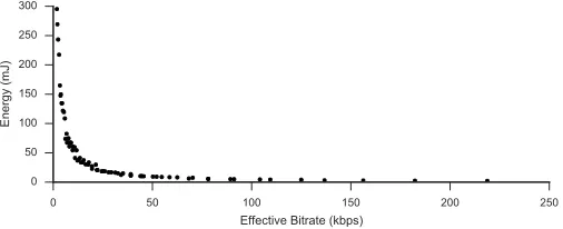
Figure 1. Effective bitrate in kilobit per second vs. energy consumption in millijoule for a packet with a 32-byte payload at 14 dBm.

the payload, but also on SF, BW, and CR. For example, a 32-byte packet at SF12, BW500 is 45 symbols large, while at SF7, BW125 it is 70 symbols large.

Investing more energy does not necessarily result in better communication performance. For example, a stronger CR is very energy costly as packets contain redundant information, however, this only leads to better communication performance in areas with burst interference. Also, similar energy consump-tion per transmission can be achieved with different parameter configurations which impact differently on communication performance.

Figure 1 shows the energy consumption for transmission of a 32 B packet at a fixed TP of 14 dBm. Each point in the graph represents a unique transmission parameter configuration using SF, BW and CR (a total of 72 combinations). The energy consumption is calculated via [7]. Depending on the setting, the energy consumption can vary from 2.20 mJ to 295 mJ, a factor of 134. Also, it can be seen that several configuration options lead to the same energy consumption. Another ob-servation is that some settings cluster and the difference in energy consumption between these is minimal. Finally, it can be observed that with increasing bitrate energy consumption reduces exponentially.

Clearly, it is desirable to select a configuration which min-imises energy consumption while supporting the application requirements in terms of network performance.

E. Transmission Parameter Selection in LoRaWAN

A LoRa gateway is able to listen for incoming transmissions concurrently on all SF and BW combinations while a device can only listen on one fixed SF and BW combination at a time. A device can therefore transmit to gateways on any combination of transmission parameters without previously agreeing on the setting. Messages transmitted from gateways to devices are transmitted on a configurable offset from the uplink data rate in the first receive window, and usually with the most robust configuration (lowest data rate) in the second receive window.

LoRaWAN provides a scheme called Adaptive Data Rate (ADR) that is used to control transmission parameter setting for the uplink from the device to the gateway. A device has the option of either selecting its data rate and transmit power individually, or have its data rate and transmit power controlled

by the network server using the ADR mechanism. A device indicates that it wants to use ADR by setting the ADR bit in the frame header.

When ADR is enabled, the network server will use the MAC commandLinkADRReqto control the end-device’s data rate and transmission power. The LinkADRReq command does not allow to select any of the 6720 potential transmission settings and provides a subset of only 8 data rate settings and 6 transmission power settings (see [8, Section 7.3.1]).

Although LoRaWAN specifies a transmission parameter signalling scheme (via the LinkADRReq command) it does not describe how the signalling should be used. It is not described how the network server should instruct devices regarding rate adaptation: when a setting should be changed, or in which order the settings should be changed. The work presented in this paper addresses this knowledge gap.

III. TRANSMISSIONPARAMETEREVALUATION

To understand the effect of the different transmission para-meters on link performance a testbed experiment is carried out. All possible parameter combinations available on our test platform are used on a single link to assess their performance impact.

A. Metrics

To evaluate link performance we use Packet Reception Rate (PRR) as metric. Most applications are able to specify network performance requirements in terms of a PRR threshold τ. A link below thresholdτ is deemed unusable by the application. A transmission parameter combination used on a link is described by a set Si = {SF, BW, CR, T P}. For each set

Si a differentP RRi is expected. EachP RRi may vary over

time as environmental conditions can change.

B. Setup

Our experimental setup consists of two NetBlocks XRange SX1272 LoRa RF modules. Sender and receiver are located in an office building, about 50 m apart separated by a number of walls. The receiving module is located in an office on the third floor; the transmitting module is located in the basement, in a separate wing of the building. The sender transmits 255 packets on each transmission setting Si (each round).

The receiver is connected to a computer, listening on the appropriate settingsSifor roundi, recording received packets

and coordinating the experiment by transmitting the settings Si+1 for the next round to the transmitter. The experiment cycles through I = 1152 settings, SF (from 7 to 12), BW (125 kHz, 250 kHz and 500 kHz), CR (4/5, 4/6, 4/7 and 4/8) and TP (2 dBm to 17 dBm). We use these I = 1152settings due to limitations of the transceiver chip.

Experiment runs are repeated over several days, during of-fice hours, and out of ofof-fice hours. An experiment run (testing allSi) took about 34 h to complete. In total, 1.6 million packets

were transmitted, of which 90.5% were received correctly, 6% were corrupt and 3.5% were lost. The reliability of the link is relatively high as for LoRa a distance of 50 m is small, even without line of sight.

C. Transmission Parameter Impact

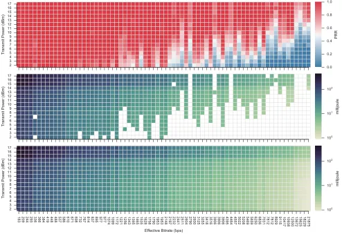
Figure 2 shows three heat maps with the averaged results of the experiments. The x-axis shows the effective bitrate, which is determined by the selected combination of SF, BW and CR according to [6]; the y-axis shows the used TP. Thus, each square in each of the heat maps corresponds to oneSi.

The heat map shown on the top depicts the PRR for each Si. The field on top-left corner with S =

{SF12,BW125,4/8,17 dBm}is the most robust transmission setting and aP RR= 1is achieved (red colour). The settings are less robust towards the right-hand side and the bottom-right corner withS={SF7,BW500,4/5,2 dBm}which represents the settings with the highest bitrate, lowest transmit power, but least robust transmission settings. Consequently PRR in this area is zero. As it can be seen, PRR is not homogeneous distributed over the graph. For some settings a low PRR is observed which improves again when changing settings to a higher effective bitrate and sometimes also lower transmission power. However, as expected, there is an area in the lower-right corner of the heat map where PRR drops off sharply.

The heat map shown on the bottom depicts the energy consumption for each setting Si. The field on the top-left

corner has the highest energy consumption per transmission of a 32 B packet (darkest colour). The bottom-right setting has the lowest energy consumption per packet. However, it has to be noted that the energy consumption per transmission does not increase linearly from the top-right to bottom-left corner. The heat map shown in the middle is a combination of the top (PRR) and bottom (energy consumption) graph. It shows the energy consumption of all settings in which a PRR above a threshold of τ = 0.9 is achieved. If we assume that the application can tolerate a link quality of up to a PRR of 0.9 the heat map shows all potentially valid transmission settings that can be used for the link.

D. Temporal Stability

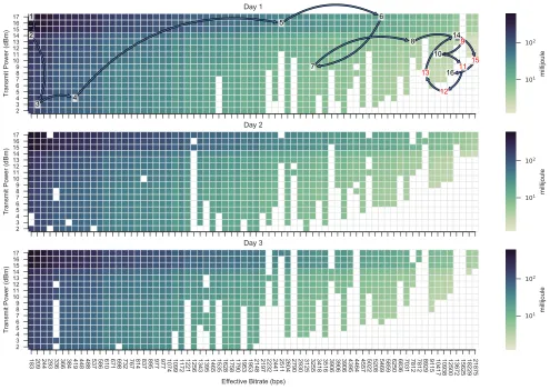
Figure 3 shows three heat maps similar to the middle heat map in Figure 2 for three different days. These heat maps show the energy consumption of all settings in which a PRR above a threshold of τ = 0.9 is achieved for three different times. It can be seen that the link changes over time and that the required PRR can be achieved with different transmission parameter settings at different times. Selecting a setting Si

must therefore take into account these temporal changes.

E. Optimal Parameter Selection

Using a full link characterisation as shown in Figure 2 allows us to pick the optimal transmission parameter config-uration. For the link shown in Figure 2, the optimal setting is

S={SF7,BW500,4/5,14 dBm}if we assume an application requirement of a PRR above a threshold of τ = 0.9. For this set of parameters the energy consumption per packet transmission is minimised.

Figure 4 shows the energy consumption per packet for the best 20 parameter settings. As it can be seen, the energy consumption per transmitted packet between the best config-uration and the next best candidates is quite small in absolute terms (resp. 2.00 mJ and 2.20 mJ). However, the difference between the optimal setting and the second best configuration is 10% which potentially translates to an increase in 10% of node lifetime (if we only consider communication related energy cost). The tenth best setting would lead to a 61% increase in energy consumption per transmission. We can therefore conclude that it is quite important to select a setting close to the optimum.

To quantify usefulness of a configuration setting Si we

define the metric δi which gives the difference in energy

consumption per packet for setting Si in relation to energy

consumption per packet for the optimal parameter settingSo:

δi= (Si/So)−1 (1)

δi is a measure of the energy waste for transmission

parameter settingSi. We define a good transmission parameter

setting as a setting which has aδibelow a threshold ofG. For

example, in a practical setting it might be considered sufficient to find a configuration withG <20%.

F. LoRaWAN Parameter Selection

Using the limited set of available LoRaWAN settings (see Section II-E), the ideal setting for this particular link would be DR6/TXPOW2 which is equivalent to S = {SF7,BW250,4/5,11 dBm}. The energy consumption for a 32 B packet is 3.21 mJ. Using our previous introduced metric to evaluate the usefulness of a selected setting we obtain δ = 61%. This shows that the available settings defined in LoRaWAN are not fine grained enough to choose good configuration settings.

G. Observations

In a practical setting it is not possible to collect data the same way as in this experiment to select a link. It is not possible to run a large number of probe transmissions on each transmission parameter setting to gather a full picture of the link. Thus it is essential to find a mechanism which is able to find a good setting S with little link probing effort that is stable over long time periods.

IV. TRANSMISSIONPARAMETERSELECTION

We propose a simple probing regime to determine a good transmission parameter setting S for a link. It is infeasible to probe a link using all possible transmission settings sequen-tially. A mechanism is necessary that can find S with little probing effort.

2 3 4 5 6 7 8 9 10 11 12 13 14 15 16 17

Transmit Power (dBm)

0.0 0.2 0.4 0.6 0.8 1.0

PRR

2 3 4 5 6 7 8 9 10 11 12 13 14 15 16 17

Transmit Power (dBm)

100

101

102

millijoule

183 209 244 293 336 366 384 419 448 488 537 586 610 671 698 732 767 814 837 895 977 977 1074 1099 1172 1221 1256 1343 1395 1465 1535 1628 1758 1790 1953 1953 2148 2197 2232 2441 2511 2604 2790 2930 3125 3255 3418 3516 3906 3906 3906 4395 4464 4557 5022 5208 5469 5859 6250 6836 7031 7812 7812 8929 9115 10417 10938 12500 13672 15625 18229 21875

Effective Bitrate (bps)

2 3 4 5 6 7 8 9 10 11 12 13 14 15 16 17

Transmit Power (dBm)

100

101

102

millijoule

Figure 2. Heatmap of transmit power and effective bitrate vs the PRR on top, and vs the energy consumption on the bottom (note the logarithmic scale). The middle figure shows the energy consumption, whereby settings with a PRR<0.9are filtered out.

report sensor readings infrequently a probing regime may take quite some time to determine a good transmission parameter settingS. Alternatively, a node may use dedicated probe trans-missions to determine S more quickly (active probing). The following discussion is independent of the specific probing regime employed (active or passive). In any case it is the aim to reduce the required probing effort.

A. Probing Algorithm

The proposed probing algorithm chooses the next probe configuration setting based on transmission energy. Other schemes are possible and are potentially more efficient. How-ever, the described approach provides good results as we will demonstrate.

Algorithm 1 describes the probing regime. Input to the algorithm is a starting setting Sm and PRR thresholdτ; the

algorithm aims to find a good setting S that is returned when the algorithm terminates. The algorithm tests a new potential setting St that uses at most half the energy of the current

settingSm. IfSthas a PRR above the thresholdτ,Stbecomes

the current setting Sm. A new setting St is picked from

all potential settings S that uses at most half of the energy of the current setting, and has not been tried before. If St

has a PRR below threshold τ, the setting S with an energy

consumption between the current (valid) setting Sm and the

tested (invalid) setting St, which has not been tried before,

is picked, and the process repeats. The algorithms continues until no more potential settings can be found. In the worst case, when there are no working settings, the algorithm will try out every possible setting. It may therefore be advantageous to set a limit on the number of iterations, or set an energy budget on what one can spend on probing.

A run of the algorithm on experimental data is shown in Fig-ure 3. The algorithm terminates after evaluating 16 transmis-sion configuration settings. The configuration chosen is S = {SF8,BW500,4/5,8 dBm} which consumes 2.31 mJ and is close to optimal setting ofSo={SF7,BW500,4/5,11 dBm}

which consumes 1.60 mJ (δi = 44%). Using the collected

testbed data it is demonstrated that the algorithm works as intended. However, it is still assumed that at each of the 16 evaluation points PRR is computed using 255 probes. In the next paragraphs we show that the number of probes at each setting can be drastically reduced.

B. Required Number of Probe Transmissions

2 3 4 5 6 7 8 9 10 11 12 13 14 15 16 17

Transmit Power (dBm)

1

2

3 4

5 6

7

8 9

10 11

12 13

14

15 16

Day 1

101

102

millijoule

2 3 4 5 6 7 8 9 10 11 12 13 14 15 16 17

Transmit Power (dBm)

Day 2

101

102

millijoule

183 209 244 293 336 366 384 419 448 488 537 586 610 671 698 732 767 814 837 895 977 977 1074 1099 1172 1221 1256 1343 1395 1465 1535 1628 1758 1790 1953 1953 2148 2197 2232 2441 2511 2604 2790 2930 3125 3255 3418 3516 3906 3906 3906 4395 4464 4557 5022 5208 5469 5859 6250 6836 7031 7812 7812 8929 9115 10417 10938 12500 13672 15625 18229 21875

Effective Bitrate (bps)

2 3 4 5 6 7 8 9 10 11 12 13 14 15 16 17

Transmit Power (dBm)

Day 3

101

102

millijoule

Figure 3. Heatmap of transmit power and effective bitrate vs energy consumption for three different days (note the logarithmic scale). All settings with a PRR<0.9are filtered out. The top graph shows the a run of the probing algorithm. Numbers indicate which settings are tested. Black numbers are above thresholdτ, red numbers are below thresholdτ(e.g. step 9, 11, 15).

0.0 2.5 5.0 7.5 10.0 12.5 15.0 17.5 20.0

Rank 0.0

0.5 1.0 1.5 2.0 2.5 3.0 3.5 4.0

Energy (mJ)

Figure 4. Energy consumption for sending a 32 B packet using the 20 best settings, havingP RR >0.9.

achieved by limiting the number of probe transmissions for each tested setting. The question is what a sensible numberN of probe transmissions is.

We evaluate the impact of different N on the quality of the

0 16 32 48 64 80 96 112 128 144 160 176 192 208 224 240 256

Probes 0.3

0.2 0.1 0.0 0.1 0.2 0.3 0.4 0.5

i

Day 1 Day 2 Day 3

found solution (as expressed via energy waste δdescribed by Equation 1) by using data collected on all settings at three different days as shown in Figure 3. From the probe trace of 255 probes we select randomly N probes and execute our algorithm. For eachN, 16 experiment runs are executed; the results are shown in Figure 5. Clearly, reducing the number of probes has an impact on the quality of the found solution. However, with increasing number of probes the impact on the quality of the solution diminishes. Using more than N = 24 probes has little impact on the result of the algorithm.

It has to be noted thatδcan be negative as shown in Figure 3 for day 3. This situation arises as the algorithm picks a setting S which does not fulfil the requirement of τ >0.9; too few probes are taken to identify a link as having an unsuitable performance.

C. Early Termination of Probing Sequence

In the previous paragraph we have shown that there is a numberN of probe transmissions that is sufficient. However, in many cases it is not necessary to transmit all N probes to determine if the threshold τ is met or not. When during probing NLprobes are already lost such that NL/N < τ it is

not necessary to complete the probe sequence and a bad link is identified early. Probing can also be terminated early when PRR is well above τ. We use the Received Signal Strength Indicator (RSSI) of a received probe to determine this case.

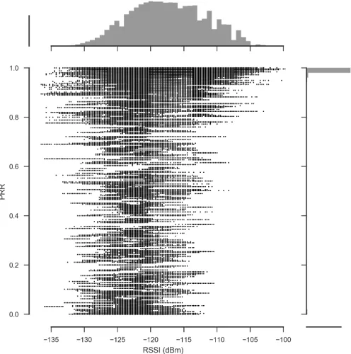
Existing work has shown that a high RSSI can be used as indicator of a very good link [9]. Figure 6 shows a plot of RSSI in relation to PRR for the packets received during the experiment described in Section III-C (Figure 2). As can be seen, a link with a PRR close to 1 has a high RSSI; however, a link with a low PRR exhibits no clear correlation with RSSI. We use this insight to improve probing and probing is terminated as soon as a probe packet with an RSSI above a threshold ofσis received. When terminating on this condition the link is assumed to provide the required reliability. For the hardware configuration used in our experiments we use σ=−105 dBm.

Algorithm 1 Probing Algorithm

1: function PROBE(τ,Sm)

2: V ← ∅

3: St←Sm

4: loop

5: V ←V ∪ {St}

6: ifPRR(St)> τ then

7: Sm←St

8: e←E(Sm)/2

9: else

10: e←(E(Sm) +E(St))/2

11: C← {x|x∈S, x6∈V, E(x)< e}

12: ifC=∅then

13: returnSm

14: else

15: St←max({E(t) :t∈C})

Figure 6. Scatter plot of RSSI vs PRR for all received packets. The plots on the axes shows a histogram of the RSSI on the x-axis, and of the PRR on the y-axis.

Using the experiment described in Section III-C (Figure 2), and N = 24, early probing termination reduces the number of transmitted probes from 384 to 285, saving 26% of the probing effort. The algorithm finds the exact same solution as without early termination and therefore there is no penalty in terms of the quality of the found solution.

D. Temporal Dynamics

We have shown in Section III-D that link conditions vary over time. The parameter selection algorithm will find a good setting S at a given point in time. However, link conditions may change and the current selected setting may become infeasible and/or a better setting may become available. The algorithm handles temporal changes in the very same way a setting is discovered initially. When data packets (data packets also function as probe transmissions) do not reach the sink anymore the node will increase link robustness restarting the algorithm with the most robust setting. Similar, after a duration T the algorithm will continue and try to find an improved setting by restarting the algorithm.

We evaluate the handling of dynamics by using the three link conditions as shown in Figure 3. The algorithm is used on data shown in Figure 3a to determine a good settingSa.

Then we assume the link condition changes as shown in Figure 3b. When this happens the selected setting Sa is not

the optimal anymore and the algorithm moves to Sb after

sending 434 probe transmissions for 36 parameter settings with δb = 0%. Thereafter we assume the link condition

sending 570 probe transmissions for 64 parameter settings with δc= 0%.

V. RELATEDWORK

Selecting communication parameters of wireless transmit-ters to reduce energy consumption is a well researched area.

In the Wireless Sensor Networks (WSN) research domain a large amount of research has been undertaken that investigates transmission power control to reduce transmission energy con-sumption (examples are [10], [11], [12]). Typical transceivers used for WSNs only provide transmission power as means to influence energy consumption. Existing algorithms to adjust transmission power depend on probe transmissions; often data transmissions double as probe transmissions. Link quality is either determined by counting lost/erroneous packets over time and/or by estimation using RSSI or Link Quality Indicator (LQI). Depending on the current link quality, transmission power is adjusted. We follow in our work these established principles. However, LoRa transceivers as used in this work provide additional parameters to influence communication energy cost which we take into account.

Previous work on WiFi and cellular networks has invest-igated either transmit power control (e.g. [13], [14], [11]), transmit rate control (e.g. [15], [16], [17]), or a combination of the two as ‘joint transmit power and rate control’ (e.g. [18], [19], [20]. Most of the transmit power control is concerned with increasing the capacity, and not necessarily the energy consumption, with the exception of [21]. The transmit rate control is often only concerned with maximising throughput. Compared to LoRa, WiFi data rates and packet rates are signi-ficantly higher, and the control algorithms run at a much higher rate then what is feasible with LoRa. For example, the most commonly used transmit rate control algorithm Minstrel [16] evaluates its links every 100 ms.

VI. CONCLUSIONS

Low-Power Wide-Area Network (LPWAN) technologies such as Long Range (LoRa) are considered for IoT deploy-ments. Networks are organised as star networks and all nodes can reach a sink in one hop. The need of constructing and maintaining a complex multi-hop network is removed but new complexity is introduced as LoRa devices can choose from 6720 transmission parameter combinations. As we have shown it is crucial to find a good transmission parameter setting such that network performance and energy consumption is balanced. We have introduced an algorithm that can find quickly a good setting, reducing the required probing effort of the link. We have shown that with 285 probes a setting can be found which uses only 44% more energy than the optimal setting (using our experimental setup). The described mechanism can be added to LoRaWAN which provides for such mechanism but does not provide any implementation details. Our next step is to deploy the mechanism in our LoRa testbed to evaluate its performance under realistic conditions.

ACKNOWLEDGEMENT

This research was partially funded through the Natural Environment Research Council (NERC) under grant number NE/N007808/1.

REFERENCES

[1] “LoRa,” https://www.lora-alliance.org/What-Is-LoRa/Technology. [2] “Sigfox,” http://www.sigfox.com.

[3] “Weightless,” http://www.weightless.org.

[4] J. Aerts, “Integrating long range technology into the contiki operating system framework,” Master’s thesis, Vrije Universiteit Brussel, June 2016.

[5] M. Bor, J. Vidler, and U. Roedig, “LoRa for the Internet of Things,”

in Proceedings of the 2016 International Conference on Embedded

Wireless Systems and Networks, ser. EWSN ’16. USA: Junction

Publishing, 2016, pp. 361–366.

[6] AN1200.22 LoRa Modulation Basics, Revision 2, Semtech, May 2015.

[7] “LoRa Calculator,” http://www.semtech.com/apps/filedown/down.php? file=SX1272LoRaCalculatorSetup1\%271.zip.

[8] N. Sornin, M. Luis, T. Eirich, T. Kramp, and O. Hersent, “LoRaWAN specification v1.0,” January 2015.

[9] N. Baccour, A. Koubˆaa, L. Mottola, M. A. Z´u˜niga, H. Youssef, C. A. Boano, and M. Alves, “Radio link quality estimation in wireless sensor networks: A survey,” ACM Trans. Sen. Netw., vol. 8, no. 4, pp. 34:1– 34:33, Sep. 2012.

[10] L. H. Correia, D. F. Macedo, A. L. dos Santos, A. A. Loureiro, and J. M. S. Nogueira, “Transmission power control techniques for wireless sensor networks,”Computer Networks, vol. 51, no. 17, pp. 4765 – 4779, 2007.

[11] S. Lin, F. Miao, J. Zhang, G. Zhou, L. Gu, T. He, J. A. Stankovic, S. Son, and G. J. Pappas, “Atpc: Adaptive transmission power control for wireless sensor networks,”ACM Trans. Sen. Netw., vol. 12, no. 1, pp. 6:1–6:31, Mar. 2016.

[12] B. Z. Ares, P. G. Park, C. Fischione, A. Speranzon, and K. H. Johansson, “On power control for wireless sensor networks: System model, middleware component and experimental evaluation,” in 2007

European Control Conference (ECC), July 2007, pp. 4293–4300.

[13] J. P. Monks, J. P. Monks, V. Bharghavan, and W.-m. W. Hwu, “A power controlled multiple access protocol for wireless packet networks,” vol. 2001, pp. 219–228, 2001.

[14] A. Muqattash, A. Muqattash, and M. Krunz, “A single-channel solution for transmission power control in wireless ad hoc networks,”IN PROC.

OF ACM MOBIHOC, vol. 2004, pp. 210–221, 2004.

[15] M. Lacage, M. H. Manshaei, and T. Turletti, “Ieee 802.11 rate adapta-tion: A practical approach,” inProceedings of the 7th ACM International Symposium on Modeling, Analysis and Simulation of Wireless and

Mobile Systems, ser. MSWiM ’04. New York, NY, USA: ACM, 2004,

pp. 126–134.

[16] D. Smithies. (2009, May) Minstrel. [Online].

Avail-able: https://sourceforge.net/p/madwifi/svn/HEAD/tree/madwifi/trunk/ ath rate/minstrel/minstrel.txt

[17] S. H. Y. Wong, H. Yang, S. Lu, and V. Bharghavan, “Robust rate adaptation for 802.11 wireless networks,” in Proceedings of the 12th

Annual International Conference on Mobile Computing and Networking,

ser. MobiCom ’06. New York, NY, USA: ACM, 2006, pp. 146–157. [Online]. Available: http://doi.acm.org/10.1145/1161089.1161107 [18] K. Ramachandran, R. Kokku, H. Zhang, and M. Gruteser, “Symphony:

Synchronous two-phase rate and power control in 802.11 wlans,”

in Proceedings of the 6th International Conference on Mobile

Systems, Applications, and Services, ser. MobiSys ’08. New

York, NY, USA: ACM, 2008, pp. 132–145. [Online]. Available: http://doi.acm.org/10.1145/1378600.1378616

[19] A. Subramanian and A. H. Sayed, “Joint rate and power control algorithms for wireless networks,” IEEE Transactions on Signal

Pro-cessing, vol. 53, no. 11, pp. 4204–4214, Nov 2005.

[20] P. Chevillat, P. Chevillat, J. Jelitto, and H. L. Truong, “Dynamic data rate and transmit power adjustment,”IEEE 802.11 Wireless LANs. Intl.

Journal of Wireless Information Networks, 2005.