First order marginalised transition random effects models with probit link function

First-order marginalised transition random e

ff

ects models

with probit link function

¨

Ozg¨ur Asar

_{, Ozlem Ilk}

a

_{CHICAS, Medical School, Lancaster University, UK}

b

_{Department of Statistics, Middle East Technical University, Turkey}

July 10, 2015

Abstract

Marginalised models, also known as marginally specified models, have recently become a popular tool for analysis of discrete longitudinal data. Despite being a novel statistical method-ology, these models introduce complex constraint equations and model fitting algorithms. On the other hand, there is a lack of publicly available software to fit these models. In this paper, we propose a three-level marginalised model for analysis of multivariate longitudinal binary out-come. The implicit function theorem is introduced to approximately solve the marginal constraint equations explicitly. probit link enables direct solutions to the convolution equations. Parameters are estimated by maximum likelihood via a Fisher-Scoring algorithm. A simulation study is con-ducted to examine the finite-sample properties of the estimator. We illustrate the model with an application to the data set from the Iowa Youth and Families Project. The R packagepnmtremis prepared to fit the model.

Keywords: correlated data, implicit differentiation, link functions, maximum likelihood estimation, subject-specific inference, statistical software.

1

Introduction

Longitudinal data comprise repeated measurements on the same subjects across time. Whilst data

from the same subjects are typically dependent on each other, data from different subjects are

typ-ically independent. Often, multiple responses, e.g. multiple health outcomes or distress variables, from each subject are collected. These responses introduce two types of dependencies: 1) within-response (serial) dependence, and 2) multivariate within-response dependence at a given time point. To draw valid statistical inferences, both of these dependencies should be taken into account.

Conventional models for analysis of longitudinal data are marginal, transition and random effects

models (Diggle et al., 2002). A recently popular method for discrete longitudinal data analysis is the framework of marginalised models, also known as marginally specified models. The framework typ-ically combines the underlying features of the conventional models, and enables likelihood-based

inference for marginal mean parameters. Heagerty and Zeger (2000) define marginally specified

models as a re-parameterised version of transition and/or random effects models in terms of the

marginal mean and additional dependence parameters. Heagerty (1999, 2002), in his seminal

pa-pers, develops marginalised random effects and marginalised transition models, respectively. Both

of these models are two-level logistic regression models. Whilst covariate effects are captured in the

first levels, serial dependence is captured in the second levels via random effects and response

his-tory, respectively. Heagerty and Kurland (2001) show that marginal regression parameter estimates

based on marginalised random effects models are less sensitive to dependence structure

misspecifi-cation compared to those based on conventional random effects models. Heagerty (2002) and Lee

and Mercante (2010) prove that parameters of the first and second levels of marginalised transition models are orthogonal. The marginalised modeling paradigm was primarily developed for binary data (Schildcrout and Heagerty, 2007; Ilk and Daniels, 2007; Lee et al., 2009; along with the

afore-mentioned works of Heagerty). Later, it has been extended to ordinal (Caffo and Griswold, 2006;

Lee and Daniels, 2007; Lee et al., 2013), count (Lee et al., 2011; Iddi and Molenberghs, 2012) and nominal data (Lee and Mercante, 2010). Amongst these works, Ilk and Daniels (2007) pro-pose a three-level marginalised model for multivariate longitudinal binary data, called marginalised

transition random effects model. With this model, whilst covariate effects are captured in the first

level, serial and multivariate response dependencies are captured in the second and third levels via

response history and random effects, respectively. In this paper, we extend marginalised transition

random effects model in terms of link function, from logit to probit, and the parameter estimation

methodology, from Bayesian methods (BM) to maximum likelihood (ML) estimation.

probit and logit are popular link functions for modelling categorical data. These link functions

are defined as the inverses of the distribution functions of the standard normal and the standard logistic distribution, respectively. They have similar behaviours in terms of placing probabilities.

The only difference is at the extreme tails; logit places higher probabilities at the tails (Hedeker and

Gibbons, 2006). Nonetheless, substantial and high quality data are needed to detect the difference

(Doksum and Gakso, 1990, cited in Hedeker and Gibbons, 2006, pp. 153). logit allows direct in-terpretation of the parameter estimates, as changes in (log) odds ratios. The inin-terpretation is more challenging with probit. Nonetheless, (approximate) transitions between the parameter estimates based on these link functions is possible (Agresti, 2002; Griswold et al., 2013). For example, the JKB constant (Johnson et al., 1995, pp. 113-163, cited in Griswold et al., 2013) postulates the

fol-lowing:βlogit c∗βprobitwhere c=(15/16)(π/

√

3)_{1.700437. One advantage of probit over logit}

is that it allows explicit form of the linkage between the levels of marginalised random effects

mod-els (Heagery and Zeger, 2000; Griswold et al., 2013; Caffo and Griswold, 2006). The use of probit

link in multivariate modelling dates back to Ashford and Sowden (1970). Some recent examples on longitudinal mixed modelling are Hedeker and Gibbons (2006), Liu and Hedeker (2006), Varin and Czado (2010), amongst others.

Generalized estimating equations (GEE; Liang and Zeger, 1986) have been widely used to esti-mate the parameters of marginal models, especially for discrete outcome. Nonetheless, they might

be inefficient because of being a semi-parametric method, compared to the full likelihood-based

methods, e.g. ML and BM. BM are widely used in longitudinal data literature and have their own properties. Some distinguishing features of ML over BM are that parameter estimation requires less computational times, and related procedures are more automatised (Efron, 1986). In this paper, we consider ML for parameter estimation to avoid the computational burden.

problems. In this paper, we consider approximately explicit solutions of marginal constraint equa-tions, and propose the use of the implicit function theorem for the first time in the scope of marginally specified models.

Publicly available software for analysis of multivariate longitudinal binary data is still rare.

Available options include the SAS macro of Shelton et al. (2004), and the R(R Core

Develop-ment Team, 2015) packagesmmm(Asar and Ilk, 2013) andmmm2(Asar and Ilk, 2014). In this study,

we propose the R packagepnmtremfor first-order marginalised transition random effects models

with probit link. The package is available from the Comprehensive R Archive Network (CRAN) at

http://CRAN.R-project.org/package=pnmtrem.

The paper is organized as follows. Whilst the general modelling framework is introduced in Section 2, first-order version is discussed in detail in Section 3. In Section 4, we discuss inference for the first-order model. Finite-sample behaviours of the estimator are investigated by a simulation study in Section 5. The first-order model is applied to a real data set in Section 6. Section 7 is a concluding discussion.

2

General framework

Let Yit jdenote the jth ( j=1, . . . ,k) response of the ith (i=1, . . . ,n) subject at time t (t=1, . . . ,T ).

Also let Xit jdenote the associated set of covariates, which might include time-varying and/or

time-invariant covariates. The framework of the general model with inverse probit link is as follows:

Pm_{it j≡}P(Yit j=1|Xit j)= Φ(Xit jβ), (1)

Pt_{it j≡}P(Yit j=1_|yi,t₋1,j, ..,yi,t−p,j,Xit j)= Φ(∆it j+ p

X

m=1

γit j,myi,t₋m,j), (2)

Pr_{it j≡}P(Yit j=1|yi,t₋1,j, ...,yi,t₋p,j,Xit j,bit)= Φ(∆∗it j+λjbit), (3)

whereΦ(_·) is the distribution function of the standard normal.

In (1), the first level of the framework, βare marginal regression parameters. These

parame-ters measure the relationship between covariates and responses, and allow comparing covariate

sub-groups, e.g. males vs. females, without conditioning on response history and/or random effects. The

default setting assumes that intercepts and slopes are shared by different responses, i.e. we postulate

βinstead ofβj. Nonetheless, one is able to specify different intercepts and slopes for multiple

re-sponses by including in Xit jindicator variables for responses and interactions of these indicator

vari-ables with covariates, respectively. This specification provides model flexibility. We might gain in

efficiencies considerably, e.g. when the relationships between covariates and multiple responses are

not significantly different (Asar and Ilk, 2014). Another default setting is the assumption of

accom-modating only the relationship of responses with current covariates, i.e. P(Yit j =1|Xi1 j, . . . ,Xit j)=

P(Yit j =1|Xit j). Nonetheless, relationships with lagged covariates might be captured by including

covariate history in Xit j.

In (2), the second level of the framework, Markov model of order p is used to capture the

serial dependence. Here, the mth transition parameters,γit j,m, can be written in terms of covariates,

i.e. γit j,m = αt,mZit j,m = αt1,mZit j1,m+. . .+αtl,mZit jl,mfor m = 1, . . . ,p. αt f,m( f = 1, . . . ,l) are

time, covariate and order specific transition parameters. They capture the relationships between

past and current responses. Zit j,. have a form of design matrix with 1’s on the first column, and

are typically a subset of Xit j with l covariates. The form of Zit j,. permits flexibly specifying the

association structures between past and current responses. For example, if one suspects that the

the first level,αt,mare assumed to be shared across multiple responses. Response-specific transition

parameters can be specified by including in Zit j,.indicator variables for responses and interactions

of these indicator variables with response history and other covariates.

In (3), the third level of the model, multivariate response dependence and individual variations

are captured. bit’s are subject and time specific random effects coefficients that measure unobserved

heterogeneity between subjects at time t. We assume that bit ∼N(0,σ2t). bit can be rewritten as

bit=σtzi, where ziis a standard normal random variable, which is useful in numerical integration.

λj’s are response-specific parameters that scale bit with respect to the jth response, and accounts

for multivariate response dependence. We setλ1 to 1 for identifiability, and estimateλj for j =

2, . . .. Note that by specifying bit’s are time-varying, the model assumes that multivariate response

dependencies might change across time.

∆it j’s in (2) are subject, time and response specific intercepts. They take into account the

(non-linear) relationship between marginal (Pm

it j) and transition probabilities (P

t

it j). Similarly,∆∗it j’s in

(3) are subject, time and response specific intercepts that account for the (non-linear) relationship

between transition and random effects probabilities (Pr_{it j}).

We assume that conditional mean of responses given all covariates is equal to conditional mean

of responses given covariate history, i.e., E(Yit j|Xiq j,q = 1, . . . ,T ) = E(Yit j|Xis j,s ≤ t). The

as-sumption is meaningful only for exogenous covariates (covariates that do not depend on response history), but not for endogenous ones (covariates that depend on response history at time t). It is necessary for the validity of the marginal constraint equation, to be introduced later.

3

First-order model

In this study, we focus on lag-1 dependence in (2). The framework for the first-order model becomes

Pm_{it j≡}P(Yit j=1_|Xit j)= Φ(Xit jβ), (4) Pt_{it j≡}P(Yit j=1_|yi,t₋1,j,Xit j)= Φ(∆it j+γit j,1yi,t−1,j), (5) Pr_{it j≡}P(Yit j=1|yi,t₋1,j,Xit j,bit)= Φ(∆∗it j+λjbit). (6)

As before, bit ∼N(0, σ2t) and bit=ziσt, zi ∼N(0,1);λ1=1;γit j,1 = αt,1Zit j,1 = αt1,1Zit j1,1+. . .+ αtl,1Zit jl,1. Throughout, we call this framework as t≥2 model.

(5) is not valid at baseline (t=1), because there is no history data are available at this time point.

Based on this and the assumption that variabilities at t=1 and t_≥1 might be different, we postulate

a separate model for t=1:

Pm_{i1 j≡}P(Yi1 j=1_|Xi1 j)= Φ(Xi1 jβ∗), (7) Pr_{i1 j≡}P(Yi1 j=1|Xi1 j,bi1)= Φ(∆∗i1 j+λ∗jbi1), (8)

where bi1∼N(0,σ21) and bi1=ziσ1, zi∼N(0,1);λ∗1=1. Throughout we call this model as the baseline

model.

3.1

Linking levels of the t

_≥

2 model

3.1.1 Linking first and second levels

Levels 1 (4) and 2 (5) are linked via the following marginal constraint equation,

P(Yit j=1|Xit j)=

1 X

yi,t−1,j=0

P(Yit j=1|yi,t₋1,j,Xit j)P(yi,t₋1,j|Xi,t₋1,j), (9)

which is equivalent to

Φ(Xi2 jβ)= Φ(∆i2 j)(1−Φ(Xi,1,jβ∗))+ Φ(∆i2 j+γi2 j,1)Φ(Xi,1,jβ∗), (10)

and

Φ(Xit jβ)= Φ(∆it j)(1−Φ(Xi,t₋1,jβ))+ Φ(∆it j+γit j,1)Φ(Xi,t₋1,jβ). (11)

for t > 2 and t = 2, respectively. Hereafter, the discussion will be based on (11). We take the

difference between (11) and (10) when necessary.

Since (11) does not permit explicitly writing ∆it j in terms ofβandγit j,1 (orαt,1), we use the

implicit function theorem (IFT; Krantz and Parks, 2003) for an approximately explicit solution. Application of IFT is as follows.

Let F be a function of Xit j, Xit−1 j,β,∆it j,αt,1and Zit j,1such that (by rewriting (11))

F(Xit j,Xit−1 j,β,∆it j,αt,1,Zit j,1)= Φ(Xit jβ)−Φ(∆it j)(1−Φ(Xi,t−1,jβ))−Φ(∆it j+αt,1Zit j,1)Φ(Xi,t−1,jβ)=0. (12)

By IFT with first order implicit differentiation, i.e. first order approximation,∆it jcan be obtained as

∆it j =−

∂F ∂β

_(β

0,αt,10,∆it j0)

∂F ∂∆it j

_(β

0,αt,10,∆it j0)

(β₋β₀)₋

∂F ∂αt,1

_(β

0,αt,10,∆it j0)

∂F ∂∆it j

_(β

0,αt,10,∆it j0)

(αt,1−αt,10), (13)

where

∂F

∂β =Xit jφ(Xit jβ)+ Φ(∆it j)(φ(Xi,t−1,jβ))Xi,t−1,j−Φ(∆it j+αt,1Zit j,1)φ(Xi,t−1,jβ)Xi,t−1,j,

∂F

∂∆it j =−φ(∆it j)(1−Φ(Xi,t−1,jβ))−φ(∆it j+αt,1Zit j,1)(Φ(Xi,t−1,jβ)),

∂F

∂αt,1

=₋φ(∆it j+αt,1Zit j,1)Φ(Xi,t−1,jβ)Zit j,1. (14)

Here, φ(_·) is the density function of the standard normal, andβ₀,αt,10 and∆it j0 are fixed values

around which IFT searches for solution. We setβ₀andαt,10to 0, since null hypotheses forβand

αt,1 are on equality of these parameters to 0. ∆it j0 is obtained by solving (12) underβ0 andαt,10

being 0. This yields∆it j0=0 for t>2. N-R is used to obtain∆i2 j0. Based on our experience, this

has very fast convergence due to the simple form of (12).

3.1.2 Linking second and third levels

Level 2 (5) and level 3 (6) are linked via the following convolution equation:

P(Yit j =1_|yi,t₋1,j,Xit j)=

Z

which is equivalent to

Φ(∆it j+αt,1Zit j,1yi,t−1,j)=

Z

Φ(∆∗_{it j}+λjbit) f (bit)dbit. (16)

Following Griswold (2005), we can explicitly obtain∆∗

it jas

∆∗_{it j}=

q

1+λ2

jσ

2

t (∆it j+αt,1Zit j,1yi,t−1,j). (17)

Proof of (17) is given in Appendix A.∆∗

it jis now an explicit and deterministic function of∆it j(hence,

∆∗

it jis a function of Xit j, Xi,t−1,jandβ),αt,1Zit j,1, yit−1 j,λjandσt.

3.2

Linking levels of the baseline model

First (7) and second (8) levels of the baseline model are linked via the following convolution equa-tion:

P(Yi1 j=1_|Xi1 j)=

Z

P(Yi1 j=1_|Xi1 j,bi1)dF(bi1). (18)

∆∗_{i1 j}can be written as an explicit function of Xi1 j,β∗,λ∗_jandσ1such that

∆∗_{i1 j}=

q

1+λ∗

j

2_σ2

1 Xi1 jβ∗. (19)

Proof of (19) can be easily adapted from the proof of (17).

4

Inference

4.1

Estimation

The likelihood of the first-order model is the product of the likelihood functions of the baseline and

t _≥2 models. By re-writing the random effects coefficients as bi1 =σ1ziand bit =σtzi, it can be

expressed as

L(θ_|y)=L1(θ1|y1)L2(θ2|y2), (20) where

L1(θ1|y1)=

N

Y

i=1

Z k

Y

j=1

Pr_{i1 j}yi1 j1₋P_{i1 j}r 1−yi1 jφ(zi)dzi, (21)

L2(θ2|y2)=

N

Y

i=1

T

Y

t=2

Z k

Y

j=1

Pr_{it j}yit j1₋P_{it j}r 1−yit jφ(zi)dzi. (22)

Here,θ=(θ1,θ2), whereθ1 =(β∗,λ∗, σ2₁) withλ∗=(λ∗₂, . . . , λ∗_k) andθ2 =(β,αt,1,λ,σ2) withλ= (λ2, . . . , λk) andσ2=(σ2₂, . . . , σ2_T), are parameters of the baseline and t≥2 models, respectively; y1

and y2are observed responses at baseline and t≥2 time points, respectively. L1(θ1|y1) and L2(θ2|y2)

are connected to each other viaβ∗at t =2 (see (10)). We model log(σt), instead ofσtorσ2t, due

to computational aspects. This transformation helps extending the parameter spaces from [0,+_∞)

to (_−∞,+_∞). Estimates and standard errors regardingσt or σ2t can be easily obtained using the

We need to use numerical methods to solve the integrals in (21) and (22), since there is no closed-form solutions. Since these integrals are one-dimensional, we use Gauss-Hermite quadrature

with 20-points (Lesaffre and Spiessens, 2001; Agresti, 2002; McCulloch et al., 2008). Similarly,

the closed-form solutions based on the first partial derivatives of the log-likelihood are not available. We use Fisher-Scoring (F-S) algorithm to obtain the parameter estimates iteratively. An advantage of F-S algorithm is that it only works with the first partial derivates and does not require the second partial derivatives (Hedeker and Gibbons, 2006, pp. 162-165). Another advantage of the algorithm is that at convergence, inverse of the expected information matrix is a consistent estimator of the large sample variance-covariance matrix of the model parameters. With F-S algorithm, ML estimates are obtained iteratively as

θ(m_s +1)=θm_s +I(θm_s)−1∂log Ls(θ

m s|ys)

∂θm_s , (23)

where s = (1,2); s = 1 corresponds to the baseline model and s = 2 corresponds to the t _≥ 2

model; m represents the F-S step and I(θs) is an empirical information matrix; ∂log(Ls(θs|ys))

∂θs is the

first partial derivative of the log-likelihood, calculations of which can be found in Appendix B. I(θs)

is calculated as

I(θ1)=

N

X

i=1

h(Yi1 j_|θ1)−2

∂h(Yi1 j_|θ1) ∂θ1

! _{∂h(Yi1 j} |θ1) ∂θ1

!T

(24)

and

I(θ2)=

N

X

i=1       

T

X

t=2 1

h(Yit j|θ2)

∂h(Yit j_|θ2) ∂θ2

             

T

X

t=2 1

h(Yit j|θ2)

∂h(Yit j_|θ2) ∂θ2

      

T

. (25)

Details of h(Yit j|θs) and ∂h(Yit j|θs)

∂θs for t = 1, . . . ,T can be found in Appendix B. Sinceσ1 is

time-specific andλ∗

jis response-specific for baseline, andσtandαt,1are time-specific andλjis

response-specific for t_≥2, the calculations of I(θ1) and I(θ2) for these parameters are different compared to

the calculations forβ∗andβ. Details can be found in the online supplementary material.

4.2

Prediction

Predicting bit =σtzi (t=1, . . . ,T ) is equivalent to predicting zi. We obtain the predictions of zi’s

as the modes of log-conditional distributions of zi’s given the data (Heagerty, 1999). This requires

solving

        

T

X

t=1

k

X

j=1 ˆ

λjσˆtφ( ˆdit j)

Yit j−Φ( ˆdit j)

Φ( ˆdit j)1₋Φ( ˆdit j)         

−zi=0, (26)

with respect to ziusin N-R algorithm. Here, ˆdit j =∆ˆ∗_{it j}+λˆjσˆtzi. ˆ∆∗_{it j}’s are obtained as in (17) and

(19) plugging-in the ML estimates ofθ1andθ2.

5

Simulation study

include bivariate binary responses, Y1 and Y2, and two associated covariates, X1 and X2, for 250

subjects with 4 follow-ups. We generate X1 from Uniform(0,1) as a time-independent variable.

X2 is taken as the response indicator variable. It takes 1 for Y1, 0 for Y2. We consider different

sets of covariates for baseline and t_≥2. Moreover, we consider varying relationships between the

covariates and the responses, i.e. β∗ .β. We specifically considerβ∗ =(β∗

0, β∗1)=(−0.5,0.5) for

t =1, andβ= (β0, β1) =(−0.7,0.7,0.2) for t =2,3,4. By the inclusion of response indicator as

a covariate, we allow the responses to have different intercepts. Whilst the intercept isβ0+β2 =

−1+0.2 =₋0.8 for Y1, it isβ0 =−1 for Y2. The relationships between X1 and Y1, and X1 and Y2

are assumed to be the same, i.e. interaction between X1and X2is not included. In terms association

structures, by keeping the marginal mean parameter setting same, we consider the following four cases:

Case 1

(λ∗

2, λ2)=(0.9,0.95), (σ1, σ2, σ3, σ4)=(0.2,0.25,0.3,0.35), (α21,1, α31,1, α41,1)=(0.3,0.4,0.5) Case 2

(λ∗

2, λ2)=(1.1,1.15), (σ1, σ2, σ3, σ4)=(0.2,0.25,0.3,0.35), (α21,1, α31,1, α41,1)=(0.3,0.4,0.5) Case 3

(λ∗

2, λ2)=(0.9,0.95), (σ1, σ2, σ3, σ4)=(0.5,0.55,0.6,0.65), (α21,1, α31,1, α41,1)=(0.3,0.4,0.5) Case 4

(λ∗

2, λ2)=(0.9,0.95), (σ1, σ2, σ3, σ4)=(0.2,0.25,0.3,0.35), (α21,1, α31,1, α41,1)=(0.6,0.7,0.8)

withλ∗

1andλ1being 1. The relationships between the lag-1 and current responses are assumed to

be same for Y1and Y2, i.e. Zit j,1=[ 1 ].

Simulated data sets are analysed by the first-order model. The simulation procedure is replicated 500 times for each case. Analysis of a simulated data set (the last one) took 8.9 minutes on a PC

with 4.00 GB RAM and 3.00 GHz processor. A simulated data set and theRscript for data analysis

are available in the user manual of thepnmtrempackage.

Simulation results are displayed in Table 1. We report mean, percentage bias (Bias(%)), empiri-cal standard deviations of the parameter estimates (SD), mean of the standard errors of the parameter estimates (meSE), and coverage probabilities of the corresponding 95% confidence intervals (CP). Parameters are approximately unbiased. Empirical standar deviations of the parameter estimates and the means of the standard error estimates are close to each other. Coverage probabilities are close to the nominal level of 0.95.

6

Example: Iowa Youth and Families Project data set

6.1

Data

We apply the first-order model to the data set from the Iowa Youth and Families Project (IFYP;

Elder and Conger, 2000; Ilk, 2008). The project was conducted to investigate long-term effects of

Table 1: Simulation results based on 500 replications. For the details of the abbreviations, see the text.

β∗

0 β∗1 β0 β1 β2

True -0.500 0.500 -0.700 0.700 0.200 Mean -0.504 0.513 -0.702 0.704 0.197 Bias (%) 0.797 2.511 0.284 0.549 -1.557 Case 1 SE 0.114 0.199 0.081 0.122 0.068 meSE 0.120 0.205 0.081 0.125 0.065 CP 0.956 0.958 0.958 0.962 0.944 Mean -0.497 0.494 -0.700 0.697 0.250 Bias (%) -0.650 -1.252 0.022 -0.480 0.081 Case 2 SE 0.120 0.206 0.081 0.119 0.066 meSE 0.119 0.204 0.082 0.125 0.065 CP 0.950 0.936 0.952 0.956 0.956 Mean -0.497 0.499 -0.706 0.712 0.198 Bias (%) -0.546 -0.136 0.923 1.755 -0.924 Case 3 SE 0.125 0.220 0.077 0.120 0.063 meSE 0.123 0.211 0.083 0.129 0.063 CP 0.946 0.944 0.960 0.962 0.950 Mean -0.499 0.498 -0.703 0.701 0.201 Bias (%) -0.183 -0.338 0.358 0.176 0.456 Case 4 SE 0.116 0.195 0.082 0.125 0.063 meSE 0.122 0.211 0.083 0.128 0.063 CP 0.956 0.964 0.966 0.956 0.956

the parents and children were surveyed. At the beginning of the study, 48% of the 7th graders were male and their average age was 12.7 years.

Three main distress variables, anxiety, hostility and depression, were used to measure emotional statuses of the young people (Table 2). These variables were collected by a list of symptoms, e.g. including nervousness, shakiness, an urge to break things and feeling low in energy etc. The symp-toms were then dichomotised (Ilk, 2008). The frequencies of the dichomotised distress variables are given in Table 3. The frequencies of depression were higher compared to those of anxiety and hostility, and the frequencies of the latter variables were close to each other. For instance, almost 93% of them reported at least one depression symptom at 1989, whilst the frequencies of anxiety and hostility were 83.2%. A set of explanatory variables, thought to be related with the distress variables, were also collected (Table 2). These variables include gender, degree of negative life event experiences of the young people, e.g. having a close friend moved away permanently, finan-cial cutbacks, e.g. moving to a cheaper residence, and negative economical event experiences of their families, e.g. such as changing job for a worse one. Amongst the explanatory variables, whilst gender was time-invariant, the others were time-varying.

Table 2: Variable list of IYFP used in PNMTREM(1).

Variable Explanation Responses

anxiety whether the young person had symptoms: 0=absence, 1=presence hostility whether the young person had symptoms: 0=absence, 1=presence depression whether the young person had symptoms: 0=absence, 1=presence Covariates

gender gender of the young person: -1=male, 1=female

NLE1 first indicator variable for negative life event experiences of young people: 1=some, -1=none or many

NLE2 second indicator variable for negative life event experiences of young people: 1=many, -1=none or some

NEE whether the household had any negative economical event: -1=no, 1=yes cut1 first indicator variable for financial cutback experiences of the household:

1=between 1 and 5, -1=none or more than 5

cut2 second indicator variable for financial cutback experiences of the household: 1=more than 5, -1=none or between 1 and 5

resp1 first response indicator variable: 1=hostility, -1=anxiety or depression resp2 second response indicator variable: 1=depression, -1=hostility or anxiety time1 first indicator variable for follow-up time: 1=1991, -1=1990 or 1992 time2 second indicator variable for follow-up time: 1=1992, -1=1990 or 1991

Table 3: Frequency table of the distress variables across years.

1989 1990 1991 1992

Anxiety 375 (83.2%) 347 (76.9%) 342 (75.8%) 327 (72.5%)

Hostility 375 (83.2%) 350 (77.6%) 342 (75.8%) 328 (72.7%)

Depression 418 (92.7%) 385 (85.4%) 378 (83.8%) 386 (85.6%)

6.2

Results

We specifically build two models. Whilst the set of explanatory variables are same, the models differ

in terms of separating the lag-1 associations amongst the distress variables. Whilst the first model

(Model 1 in Table 5) assumes these associations are shared across the responses, i.e. Zit j,1 =[ 1 ],

the second model (Model 2 in Table 5) assumes that the associations are different for the distres

variables, i.e. Zit j,1 =[ 1 resp1 resp2 ]. Results for baseline models are presented in Table Table

4. Note that the baseline results of Model 1 and Model 2 are same, since the specifications of the

baseline parameter sets are same. Results for t_≥2 models are presented in Table 5.

We compare Model 1 and 2 by likelihood ratio test (LRT), since they are nested. Respective

maximised log-likelihoods are -1236.78 (=₋210.78₋1026) and -1234.49 (=₋210.78₋1023.71).

The LRT statistic is 4.58 (=₋2_∗(₋1026₋(₋1023.71))), with a p-value of 0.60. This indicates that

there is not enough evidence to conclude that Model 2 is a better model to analyse the IYFP data set compared to Model 1. Therefore, throughout the paper we only discuss the results of Model 1.

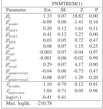
Table 4: Results for t=1989. H0 :λ∗_hostility=1 and H0:λ∗_depression=1; other parameters are tested for 0.

PNMTREM(1)

Parameter Est. SE Z P

β∗

0 1.33 0.07 18.82 0.00

β∗

gender -0.09 0.06 -1.41 0.16

β∗

NLE1 0.20 0.12 1.61 0.11

β∗

NLE2 0.41 0.12 3.27 0.00

β∗_NEE 0.03 0.05 0.72 0.47

β∗_cut1 0.08 0.07 1.15 0.25

β∗

cut2 -0.003 0.07 -0.04 0.97

β∗

resp1 -0.001 0.06 -0.02 0.99

β∗

resp2 0.29 0.07 4.17 0.00

β∗

gender∗resp1 -0.04 0.06 -0.73 0.47

β∗

gender∗resp2 -0.08 0.07 -1.29 0.20

λ∗_hostility 1.10 0.79 0.12 0.91 λ∗

depression 1.04 0.71 0.05 0.96

log(σ1) -0.41 0.41

Max. loglik. -210.78

6.3

Population-averaged results

At baseline (1989), only the intercept, one of the negative life event indicators (NLE2) and one of

the response indicators (resp2) are significant. The estimate of intercept, ˆβ∗

0 =1.33, indicates that

young people had high probability of distress at 1989. The estimate of the second response indicator variable, ˆβ∗

resp2=0.29, indicates that young people were more likely to report depression compared

to anxiety and hostility. Insignificance of the first response indicator (p-value=0.99) indicates that

reporting anxiety and hostility were equally likely. These findings are in agreement with the em-pirical frequencies (Table 3). Young people who had many negative life events were more likely

to be distressed ( ˆβ∗

NLE2 = 0.41). Pairwise correlations between anxiety, hostility and depression

were not significantly different, p-values ofλ∗

hostilityandλ∗depressionwere 0.91 and 0.96. The standard

deviation estimate of the random effects distribution is 0.66 (=exp(₋0.41)), with a standard error

of 0.27 (= p0.412_{∗exp(−0.41∗2), by the delta method). The standard deviation is significantly}

different from 0, with a p-value of 0.007. Of note, we modified the p-value following Molenberghs

and Verbeke (2007).

For 1990₋1992, the intercept, gender, both negative life event indicators (NLE1, NLE2),

nega-tive economical events experience (NEE), one of the cutbacks indicators (cut1), one of the response indicators (resp2), one of the time indicators (time2) and the interaction between gender and second

response indicator (gender * resp2) are significant. The estimate of the intercept ( ˆβ0 =0.96)

indi-cates high probability of distress for 1990₋1992, which tend to be higher compared to baseline,

since ˆβ∗

0 > β0ˆ . Females were more likely to report distress compared to males ( ˆβgender = 0.18).

Furthermore, they were more likely to report depression ( ˆβgender∗resp2=0.07) compared to reporting

anxiety or hostility. Note that gender is insignificant at 1989. This finding was also reported in Ge et al. (2001, cited in Ilk, 2008) and Ilk (2008). Experiencing many negative life events and any

family-level negative economical events were associated with distress ( ˆβNLE1=0.14, ˆβNLE2 =0.38

Table 5: Results for t_≥1990. H0 :λhostility=1 and H0:λdepression=1; other parameters are tested

for 0.

Model 1 Model 2

Parameter Est. SE Z P Est. SE Z P

β0 0.96 0.05 20.77 0.00 0.96 0.05 19.49 0.00

βgender 0.18 0.03 5.87 0.00 0.18 0.03 5.87 0.00

βNLE1 0.14 0.04 3.09 0.00 0.14 0.05 3.05 0.00

βNLE2 0.38 0.05 7.95 0.00 0.38 0.05 7.90 0.00

βNEE 0.08 0.03 3.08 0.00 0.08 0.03 3.03 0.00

βcut1 0.06 0.03 2.10 0.04 0.07 0.03 2.20 0.03

βcut2 0.02 0.03 0.72 0.47 0.02 0.03 0.73 0.47

βresp1 0.01 0.04 0.28 0.78 0.01 0.04 0.13 0.90

βresp2 0.22 0.04 5.21 0.00 0.22 0.05 4.66 0.00

βtime1 -0.07 0.04 -1.75 0.08 -0.08 0.05 -1.75 0.08

βtime2 -0.09 0.05 -1.96 0.05 -0.09 0.05 -1.88 0.06

βgender∗resp1 -0.01 0.03 -0.18 0.86 -0.01 0.03 -0.20 0.84

βgender∗resp2 0.07 0.04 2.08 0.04 0.07 0.04 2.07 0.04

βresp1∗time1 -0.002 0.03 -0.07 0.95 -0.02 0.04 -0.42 0.68

βresp1∗time2 0.004 0.04 0.10 0.92 0.003 0.04 0.07 0.94

βresp2∗time1 -0.01 0.04 -0.36 0.72 -0.01 0.04 -0.31 0.75

βresp2∗time2 0.05 0.04 1.15 0.25 0.05 0.04 1.03 0.30

α21,1 0.76 0.11 6.62 0.00 0.75 0.17 4.50 0.00

α22,1 0.06 0.13 0.43 0.67

α23,1 0.11 0.16 0.70 0.48

α31,1 0.87 0.10 9.11 0.00 0.86 0.13 6.58 0.00

α32,1 0.08 0.11 0.74 0.46

α33,1 0.07 0.14 0.48 0.63

α41,1 0.90 0.10 9.53 0.00 0.86 0.12 7.03 0.00

α42,1 -0.04 0.12 -0.34 0.74

α43,1 0.12 0.13 0.93 0.35

λhostility 1.03 0.37 0.60 0.94 0.99 0.36 -0.02 0.99

λdepression 1.21 0.49 0.57 0.68 1.18 0.49 0.36 0.72

log(σ2) -0.48 0.25 -0.47 0.26 log(σ3) -0.62 0.25 -0.59 0.26

log(σ4) -0.62 0.26 -0.59 0.26 Max. loglik -1026.00 -1023.71

( ˆβresp2 = 0.22). On the other hand, reporting anxiety or hostility were not significantly different

(p-value ofβresp1 = 0.78). Whilst the distress levels were lower at 1992 compared to 1990 and

1991 ( ˆβtime2=−0.09), the distress levels at 1990 and 1991 were not significantly different from each

other (p-value ofβresp1=0.08). The decrease in the distress probabilities at 1992 was not different

for depression, anxiety and hostility; respective p-values forβresp1∗time2andβresp2∗time2are 0.92 and

0.25.

The marginal mean parameter estimates based on probit link can be interpreted in terms of odds-ratios, using the JKB constant; for details see Introduction. For instance, young people who

experienced many negative life events were approximately 2.26 (= exp(1.700437_∗((₋1_∗0.14+

1_∗0.38)₋(1_∗0.14₋1_∗0.38)))) times more likely to be distressed compared to those with some

negative life events, and individuals in the latter group were 1.60 (=exp(1.700437_∗((1_∗0.14₋1_∗

0.38)₋(₋1_∗0.14₋1_∗0.38)))) times more likely to be distressed compared to those with no negative

life events.

The transition parameter estimates are positive and significant: ˆα21,1 = 0.76, ˆα31,1 = 0.87,

ˆ

α41,1=0.90 with p-values<1×10−10. These indicate that that young people who were distressed at

pairwise correlations between anxiety, hostility and depression were not significantly different; cor-responding p-values were 0.94 and 0.68 for hostility and depression, respectively. The standard

de-viation estimates of the random effects distributions were 0.62 (=exp(₋0.48)), 0.54 (=exp(₋0.62))

and 0.54 (= exp(₋0.62)) at 1990, 1991 and 1992, respectively. Respective standard errors were

0.16, 0.14 and 0.14, and all of these parameters were significant (p-values<0.0001). These results

indicate that the individual variations decreased through time (recall that ˆσ1=0.66) and close to each

other at 1991 and 1992.

6.4

Subject-specific results

We calculate probabilities of reporting anxiety, hostility and depression for each individual at each year. We also calculate the marginal probabilities for comparison. These probabilities are plotted in Figure 1; only the results for depression are shown here due to page limits, others can be found in the online supplementary material. We label observed values by 0 and 1 according to absence and presence depression, respectively. Marginal probabilities range in a narrower interval compared to conditional probabilities. For instance, whilst the range for the marginal probabilities of being depressed at the period of 1990 - 1992 was (0.576, 0.971), it was (0.118, 0.999) for the conditional probabilities. This indicates that marginal probabilities are high even for young people who did not report depression. On the other hand, conditional probabilities leads to correct decisions. For instance, in Figure 1, the 0’s were associated with lower conditional probabilities. The associated box-plots reflect the location and scale of the marginal and conditional probabilities. Whereas the the conditional probabilities have a spread distribution with many outliers, the marginal probabilities have a stacked and narrow distribution.

Probabilities of a young person with ID=223 are presented in Table 6. This person was a female,

with some negative life event experiences, no negative economical event experiences and cutbacks between 1 and 5, except in 1992 at which her family did not experience any cutbacks. She did not

report distress at all. Predicted value of z223is−2.45. This indicates that she was less likely to report

distress compared to an average person, i.e. zi = 0. For this person, the conditional probabilities

lead to correct inferences compared to the marginal probabilities. For instance, at 1992, whereas the marginal probability of being anxious is 0.64, the conditional probability being anxious is 0.08. We also calculate conditional probabilities assuming that the person is an average person, i.e. setting

z223=0. Related results are given under Conditional∗. These probabilities are still subject, time and

response specific, since∆∗_{it j}holds subject, time and response specific information. For instance, at

0.0 0.2 0.4 0.6 0.8 1.0 0.0 0.2 0.4 0.6 0.8 1.0 1989 marginal conditional 0 0 0 0 0 0 0 0 0 0 0 0 0 0 0 0 0 0 0 0 0 00 0 0 0 0 0 0 0 0 0 0 1 1 1 1 1 1 1 1 1 1 1 1 11 11 1 1 1 1 1 1 1 1 1 1 1 1 1 1 1 1 1 1 1 1 1₁ 1₁ 1 1 1 1 1 1 1 1 1 1 1 1 1 1 1 1 1 11 1 1 1 1 11 1 1 1 1 1 1 1 1 1 1 11 1 1 1 1 1 11 1 1 1 11

1 1

1 1 1

1 11₁1

1 1 1 1 1 1 1 11 1 1 1

1 11 1₁ 1 1 1 1 1

1 1 1 1 11 1 1 1 111

1 1 1 1 11 1

1 1 ₁ 1 1 1 1 1 1 1 1₁ 1 11 1 1 1₁ 1 1 1 1 11 1 111 1 1 1 1 111 1

111 11 1 1 1 11 1 1 1 1 1 1 1 1 1 1 1 11 1 1 1 1 1 1 1 1 1111 1 1 1 1 1 1 1 1 1 1 1 1 1 1 1 11 1111

11 1 1 1 1 1 1 1 1 1 1 1 1 1

1 11 1 1 1 1 1 1 1 11₁11 11 11

1 1 1 1 11 1

1 1 1

1 1 1 1 1 1 1 1 1 1 1 1 1 ₁ 1 1 1 1 1 1 1 1 1 1 1 1 1 11 1 1 1 1 1 1 1 1 1 1 1 1 1 1 11 1 1 1 1 1 1 1 1 1 1 1111

1 1 1 1 1 1 1 1 1 1 1 1 1 1 1 1 1 11 1 1 1 1 111 1 1 1 ₁ 1 1 1 1 1 1 1 1 1 1 1 1 1 1 1 1 1 1 1 11 1 1 1 1 1 1 1 1 1 1 1 1 11 1 1 1 1 1 1 1 1 1 1 1 11 1111

0.0 0.2 0.4 0.6 0.8 1.0

0.0 0.2 0.4 0.6 0.8 1.0 1990−1992 marginal conditional 0 0 0 0 0 0 0 0 0 0 0 0 0 0 0 0 0 0 0 0 0 0 0 0 0 0 0 0 0 0 0 0 0 0 0 0 0 0 0 0 0 0 0 0 0 0 0 0 0 0 0 0 0 0 0 0 0 0 0 0 0 0 0 0 0 0 0 0 0 0 0 0 0 0 0 0 0 0 0 0 0 0 0 0 0 0 0 0 0 0 0 0 0 0 0 00 0 0 0 0 0 0 0 0 0 0 0 0 0 0 0 0 0 0 0 0 0 0 0 0 0 0 0 0 0

0 00

0 0 0 0 0 0 0 0 0 0 0 0 0 0 0 0 0 0 0 0 0 0 0 0 0 0 0 0 0 0 0 0 0 0 0 0 0 0 0 0 0 0 0 0 0 0 0 0 0 0 0 0 0 0 0 0 0 0 0 0 0 0 0 0 0 0 0 0 0 0 0 0 0 0 0 1 1 1 1 1 1 1 1 1 1 1 1 1 1 1 1 1 1 1 1 1 1 1 1 1 1 1 1 11 1 1 1 1 1 1 1 1 1 1 1 1 1 1 1 1 1 111 1 1 1 1 1 1 1 1 1 1 1 1 1 1 1 1 1 1 1 1 1 1 1 1 1 1 1 1 1 1 1 1 1 1 1 1 1 1 1 1 1 1 1 1 1 1 1 1 1 11

1 1 1 1 1 1 1 1 11 1 1 1 1 1 1 1

1 1 1

1 1 1 1 1 1 1 1 1 1 1 1 1 1 1 1 1 1 1 1 1 1 1 1 1 1 1 1 1 1 1 1 1 1 1 1 1 1 1 1 1 1 1 1 1 1 1 1 1 1 1 1 1 1 1 1 11 1 1 1 1 1 1 1 1 1 1 1 1 1 1 1 1 1 1 1 1 1 1 1 1 1 11₁

1 1 1 1 1 1 1 1 1 1 1 1 11 1 1 1 1

1 1 1

1 1 1 1 1 1 1 1 1 1 1 1 1 1 11 1 1 1 1 1 1 1 1 1 1 1 1 1 1 11 1 11 1

1 1 1

1 1 1 1 1 1 1

1 1 1

1 1 1 1 1 1 1 1 1 1 1 1 1 1 1 1 1 1

1₁1

1 1 11 1 1 1 1 1 1 1 1 1 1 1 1 1 1 1 1 1 1 1 1 1 1 1 1 1 1 1 1 1 1 1 1 1 1 11 1 1 1 1 1 1 1 1 1 ₁ 1 1 1 1 1 1 1 1

11 1

1 1 1 1 1 1 1 1 1 1 1 1 1 1 1 1 1 1 1 1 1 1 11 1 1 1 1 1 1 1 1 1 1 1 1 1 1 1 1 1 1 1 11 1 1 1 1 1 1 1 1 1 1 1 1 11111 1

1 1 11

1 1 1 1 1 1 1 1 1 1 1 1 1 1 1

1 1 1

1 1 1 1 1 1 1 1 1 1 1 1 1 1 1 1 1 1 1 1 1 1 1 1 1 1 1 1 1 11 1 1 1 11 11 1

1

1 1111 111 1 1 1 1 1 1 11 1 1 1 1 1 1 1 1 1 1 1 1 1 1 1 1 1 1 1 1 1 1 1 1 1 1 1 1 1 1 1 1 1 1 1 1 1 1 1

1 1 1

1 1

11 1

11 1 1 1 1 1 1 1 1 111 ₁1

1 1 1 1 1 1 1 1 1 1 1 1 1 1 1 1 1 1 1 1 1 1 1 1 1

1 1 1

1 1 1 11 1 1 1 1 1 1 1 1 11 1 1 1 1 1 1 1 1 1 1 1 1 1 1 1 1 1 1 1 1 1 11 1 1 1 1 1 1 1 1 1 1 1 1 1 1 1 1 1 1

1 11

1 1 1 1 1 1 1 1 1 1 1 1 1 1 1 1 1 1 1 1 1 1 1 1 1 1 1 1

111 1 1 1 1 1 1 1 1

1 11

1 1 1 1 1 1 1 1 1 1 1 1 1 1 1 1 1 1 1 1 1 1 1 1 1 1 1 1 1 1 1 1 1 1 1 1 11 ₁ 1 1 1 1 1 1 1 1 1 1 11 1 1 1 1 1 1 1 1 1 1

11 1

1 1 1 1 1 1 1 1 1 1 1 1 1 1 1 1 1 1 1 1 1 1 1 1 1 11 1

1 1 1 1 1 1 1 1 1 1 1 1 11 111 11

1 1 1 1 1 1 1 1 1 1 1 1 1 1 11 1 1 1 1 1 1 1 1 1 1 1 1 1 1 1 1 1 1 1 1 1 1 1

1 11 1

1 1 1 1 1 1 1 1 1 1 1 ₁1 111 11

1 111

11 1 1

1 1 1 1 1 1 1 1 1 1 1 1 1 1 1 1 1 1 1 1 1 1 1 1 1

1 11

1 1

1 11 11

1 1 1 1 1 1 1 11 1 1 1 1 1 1 1 1 1 1 1 1 1 1 1

111

1 1 1 1 1 1 1 1 1 1 1 1 1 1 1 1 1 1 1 1 1 1 1 1 1 1 1 1 1 1 1 1 1 1 1 1 1 11 1 1 1 1 1 1 1 1 1 1 1 1 1 1 1 1 1 1 1 1 1 1 1 1 1 1 1 1 1 1 1 1 1 1 1 1 1 1 1 11 1 1 1 1 1

1 11

11 1

1

1 11 1

1

1

1 1 1₁

1 1 1 1 1 1 1 1 1 1 1 1 1 1 1 1 1 1 1 11 1 1 1 1 1 1 1 1 1 1 1 1 1 1 1 1 1 1 1 11 1111 1

1 1₁₁ 1

1 1 1 1 1 1 1 1 1 1 1 1 1 1 1 1 1 1 1 1 1 1 1 1 1 1 1 1 1 1 1 1 1 1 1 1 1 1 1 1 1 1 1 1 1 1

1 1 1

1 1 1 1 1 1 1 1 1 1 1 1 1

Figure 1: Scatter and box plots of marginal vs. conditional probabilities for depression at 1989 (left panel) and 1990-1992 (right panel).

1

Table 6: Marginal and conditional probabilities for the young person with ID=223.

Time Response Gender NLE NEE Cutbacks Observed Marginal Conditional Conditional∗ Anxiety Female Some No Betw. 1 & 5 Absence 0.82 0.30 0.87 1989 Hostility Female Some No Betw. 1 & 5 Absence 0.80 0.23 0.85 Depression Female Some No Betw. 1 & 5 Absence 0.91 0.47 0.95 Anxiety Female Some No Betw. 1 & 5 Absence 0.78 0.09 0.56 1990 Hostility Female Some No Betw. 1 & 5 Absence 0.78 0.09 0.58 Depression Female Some No Betw. 1 & 5 Absence 0.90 0.14 0.77 Anxiety Female Some No Betw. 1 & 5 Absence 0.74 0.14 0.59 1991 Hostility Female Some No Betw. 1 & 5 Absence 0.74 0.13 0.59 Depression Female Some No Betw. 1 & 5 Absence 0.86 0.22 0.79 Anxiety Female Some No None Absence 0.64 0.08 0.46 1992 Hostility Female Some No None Absence 0.65 0.08 0.47 Depression Female Some No None Absence 0.85 0.19 0.77

Table 7: Frequency table of the stayers. “All” stands for the subjects who reported the same answer for all the distress variables.

Absence (0) Presence (1)

Anxiety 15 (3.3%) 215 (47.7%)

Hostility 9 (2%) 221 (49%)

Depression 2 (0.4%) 288 (63.9%)

All 2 (0.4%) 134 (29.7%)

6.5

Diagnostics

Longitudinal binary data sets almost surely include stayers, i.e. subjects who constantly report

ab-sence (0) or preab-sence (1) of a binary variable at all time points, for which the subject with ID=223

is an example. The counts and percentages of the stayers in the IYFP data set are given in Table 7. For instance, 29.7% of the subjects reported 1 for all the three distress variables at all the time points. Marginal and conditional anxiety probabilities of the stayers in terms all the distress vari-ables are summarised in Figure 2. Other results can be found the online supplementary material. Whilst the gray lines represent the subjects who always reported 1, the black lines represent the ones who always reported 0. Conditional probabilities are successful at correctly assigning the success probabilities for these subjects; higher probabilities for subjects reporting 1 and lower probabilities for those who reported 0. On the other hand, marginal probabilities are not able to distinguish these subjects.

We also calculate accuracy measures to summarise the predicted probabilities. We specifically use expected proportion of correct prediction (Herron, 1999) and area under the receiver operating characteristics curve (AUROC). Results (not shown here) show that conditional probabilities

out-perform the marginal probabilities. This difference is apparent especially in terms of AUROC. For

instance, while the AUROC value for depression at 1990-1992 is 0.684 for marginal probabilities, it is 0.864 for the conditional probabilities.

7

Discussion and conclusion

Un-1989 1990 1991 1992 0.0

0.2 0.4 0.6 0.8 1.0

Marginal

1989 1990 1991 1992 Conditional

Years

Probability

Figure 2: Spagetti plots of marginal (left panel) and conditional (right panel) anxiety probabilities for stayers in terms of all the distress variables. While gray lines represent subjects who reported 1, the black lines represent subjects who reported 0.

automated Fortran codes are available from the personal website of Dr. Ilk. However, their procedure is computationally cumbersome and requires expertise in BM and Fortran. These aspects prohibit the routine use of the model. In this study, we replace logit link by probit, and use ML for parameter estimation. probit link enables us explicitly linking the second and third levels of the model, which is not possible with the logit link. On the other hand, parameter estimation with ML takes less time compared to BM. We propose the use of implicit function theorem to solve the marginal constraint equations directly. To the best of our knowledge, this application is proposed for the first time here

for marginalised models. We have prepared the publicly available R packagepnmtremto fit the

proposed model. Currently, the package provides a function for fitting the first-order model. The

function considers both parameter estimation and random effects prediction. It has been tested under

different conditions. For the details and usage, we refer the readers to the package manual.

We have conducted a simulation study to investigate the properties of the estimator under diff

er-ent scenarios. Results are satisfactory in terms of unbiasedness, efficiency and coverage. We have

illustrated the first-order model with an application to the IYFP data set. Both population-averaged and subject-specific inferences have been illustrated. Our findings on the IYFP data analysis coin-cide with the findings of Ilk (2008). As a separate note, the IYFP data set is available upon request from the authors.

A natural extension of our work here would be fitting higher-order models. The variances of

random effects could be modified by a subset of covariates, i.e. log(σt)= Mit jωt where Mit j is a

set covariates andωtare the associated parameters. Also, the random effects coefficients might be

assumed to have a multivariate normal distribution, i.e. bit ∼N(0,D) where D is a T×T matrix.

Appendices

A. Linking second and third levels of the t

_≥

2 model

Whilst linking second and third levels of the t_≥2 model, we claim the following

R

Φ(∆∗_{it j}+λjbit) f (bit)dbit= Φ

      ∆∗ it j q

1+λ2

jσ2t      

where bit ∼ N(0, σ2t) and bit = ziσt, zi ∼ N(0,1). The related proof, which is modified from

Griswold (2005), is given below.

Let Wi⊥zi, where Wi∼N(0,1), then,

Wi/(λjσt)∼N(0,(λjσt)−2) Wi/(λjσt)−zi∼N(0,1+(λjσt)−2)

Wi/(λjσt)−zi √

1+(λjσt)−2 ∼

N(0,1)

and

Z

Φ(∆∗_{it j}+λjbit) f (bit)dbit=

Z +∞

−∞

Φ(∆∗_{it j}+λjziσt)φ(zi)dzi

=

Z +∞

−∞

P(Wi_≤∆∗_{it j}+λjziσt)φ(zi)dzi

=

Z +∞

−∞ P       

Wi/(λjσt)−zi

p

1+(λjσt)−2

≤

∆∗

it j/(λjσt)

p

1+(λjσt)−2

      φ(zi)dzi

=P       

Wi/(λjσt)−zi

p

1+(λjσt)−2

≤

∆∗

it j/(λjσt)

p

1+(λjσt)−2

      = Φ

       ∆∗ it j p

1+(λjσt)2

      

B.1 ML estimation of

θ

Maximizing the log-likelihood function of the baseline model, L1(θ1|y1), with respect toθ1yields

∂log L1(θ1|y1)

∂θ1 ≈ N X

i=1

1

h(Yi1|θ1)

∂h(Yi1|θ1)

∂θ1

, (27)

where

h(Yi1_|θ1)≈ 20 X

q=1

wq exp         k X

j=1

Yi1 jlogΦ(di1 jq)

+(1₋Yi1 j)log1₋Φ(di1 jq)

       

| {z }

ℓ(Yi1|θ1)

, (28)

∂h(Yi1_|θ1) ∂θ1 ≈

20 X

q=1

wq         

ℓ(Yi1|θ1)          k X

j=1        

∂di1 jq

∂θ1

φ(di1 jq)

       

Yi1 j₋Φ(di1 jq)

Φ(di1 jq) 1−Φ(di1 jq)

                                  , (29)

di1 jq=

q

1+λ∗

j

2_e2c1_{(Xi1 jβ}∗_)+λ∗ je

c1√_{2 z}

Here, log(σ1) is equated to c1for simplicity of notation and (zq,wq) for q =1, . . . ,20 are

Gauss-Hermite quadrature points and weights, respectively which are available in Abramowitz and Stegun

(1972). The derivatives of di1 jq with respect toθ1 = (β∗,λ∗,c1) withλ∗ = (λ∗₂, . . . , λ∗_k) are given

below.

∂di1 jq

∂β∗ =

q

1+λ∗

j

2_e2c1_{(Xi1 j)} ∂di1 jq

∂λ∗

j

=(1+λ∗

j 2

e2c1₎−1/2_λ∗

je 2c1_(X

i1 jβ∗)+ec1

√ 2zq

∂di1 jq

∂c1

=(1+λ∗j

2

e2c1₎−1/2_λ∗

j 2

e2c1_(X

i1 jβ∗)+λ∗je c1√_2z

q

B.2 ML estimation of

θ

Similar to the baseline model, maximizing the log-likelihood function of the t _≥ 2 model with

respect toθ2yields

∂log L2(θ2|y2)

∂θ2 ≈ N X

i=1 T X

t=2

1

h(Yit|θ2)

∂h(Yit|θ2)

∂θ2

, (31)

where

h(Yit_|θ2)≈ 20 X

q=1

wq exp         k X

j=1

Yit jlogΦ(dit jq)

+(1₋Yit j)log1₋Φ(dit jq)

       

| {z }

ℓ(Yit|θ2)

, (32)

∂h(Yit|θ2) ∂θ2 ≈

20 X

q=1

wq         

ℓ(Yit|θ2)          k X

j=1        

∂dit jq

∂θ2

φ(dit jq)

       

Yit j−Φ(dit jq)

Φ(dit jq) 1−Φ(dit jq)

                                  , (33)

dit jq=

q

1+λ2_je2ct_{∆it j+αt,1Zit jyit}

−1 j

+λject√_2z

q. (34)

Here, ct=log(σt) for t≥2, and (zq,wq) for q=1, . . . ,20 are Gauss-Hermite quadrature points and

weights. Also note that explicit solution of∆it jis given in (13). The derivatives of dit jqwith respect

toθ2=(β,αt,1,λ,c) withλ=(λ2, . . . , λk) and c=(c2, . . . ,cT) are given below. ∂dit jq

∂β =

q

1+λj2e2ct( Ait j)

∂dit jq

∂αt,1

=

q

1+λj2e2ct(Bit j+Zit j,1yit−1 j)

∂dit jq

∂λj

=(1+λj2e2ct)−1/2λje2ct

−( Ait jβ0+Bit jαt,10)+Ait jβ+αt,1(Bit j+Zit j,1yit−1 j)

+ect√_2z

q

∂dit jq

∂ct

=(1+λj2e2ct)−1/2λj2e2ct

−( Ait jβ0+Bit jαt,10)+Ait jβ+αt,1(Bit j+Zit j,1yit−1 j)

+λject

√ 2zq

where

Ait j=− ∂F ∂β _(β

0,αt,10,∆it j0)

∂F ∂∆it j

_(β

0,αt,10,∆it j0)

, Bit j =− ∂F ∂αt,1

_(β

0,αt,10,∆it j0)

∂F ∂∆it j

_(β

References

Abramowitz, K. M. and Stegun, I. A. (1972) Handbook of mathematical functions. New York: Dover Publications.

Agresti, A. (2002) Categorical data analysis, 2nd edition. New Jersey: John Wiley & Sons.

Asar, ¨O. and Ilk, ¨O. (2013) mmm: an R package for analyzing multivariate longitudinal data

with multivariate marginal models. Computer Methods and Programs in Biomedicine, 112, 649– 654.

Asar, ¨O. and Ilk, ¨O. (2014) Flexible multivariate marginal models for analyzing multivariate

longitudinal data, with applications in R. Computer Methods and Programs in Biomedicine,

115, 135–146.

Ashford, J. and Sowden, R. (1970) Multivariate probit analysis. Biometrics, 26(3), 535–546.

Caffo, B. and Griswold, M. (2006) User-friendly introduction to link-probit-normal models.

American Statistician, 60 (2), 139–145.

Diggle, P. J., Heagerty, P., Liang, K. -Y. and Zeger, S. L. (2002) Analysis of longitudinal data, 2nd edition. Oxford: Oxford University Press.

Doksum, K. A. and Gasko, M. (1990) On a correspondence between models in binary regression analysis and in survival analysis. International Statistical Review, 58, 243–252.

Efron, B. (1986) Why isn’t everyone a Bayesian? The American Statistician, 40(1), 1–5.

Elder, G. H. and Conger, R. (2000) Children of the land. The University of Chicago Press.

Ge, X., Conger, R. D. and Elder, G. H. (2001) Pubertal transition, stressful life events, and the

emergence of gender differences in adolescent depressive symptoms. Developmental

Psychol-ogy, 37(3), 404–417.

Griswold, M. (2005) Complex distributions, hmmmm... hierarchical mixtures of marginalized

multilevel models. Ph.D. Thesis, Johns Hopkins University.

Griswold, M., Swihart, B. J., Caffo B. S. and Zeger S. L. (2013) Practical marginalized

multi-level models. Stat, 2, 129–142.

Heagerty, J. P. (1999) Marginally specified logistic-normal models for longitudinal binary data.

Biometrics, 45(3), 688–698.

Heagerty, P. and Zeger, S. L. (2000) Marginalized multilevel models and likelihood inference (with comments and a rejoinder by the authors). Statistical Science, 15(1), 1–26.

Heagerty, J. P. and Kurland, B. F. (2001) Misspecified maximum likelihood estimates and gen-eralised linear mixed models. Biometrika, 88(4), 973–985.

Heagerty, J. P. (2002) Marginalized transition models and likelihood inference for longitudinal categorical data. Biometrics, 58, 342–351.

Herron, M. (1999) Postestimation uncertainty in limited dependent variable models. Political

Analysis, 8, 83–98.

Iddi, S. and Molenberghs, G. (2012) A combined overdispersed and marginalized multilevel model. Computational Statistics and Data Analysis, 56, 1944–151.

Ilk, ¨O. and Daniels, M. J. (2007) Marginalized transition random effects models for multivariate

longitudinal binary data. The Canadian Journal of Statistics, 35, 105–123.

Ilk, ¨O. (2008) Multivariate longitudinal data analysis: models for binary response and

ex-ploratory tools for binary and continuous response. Saarbr¨ucken: Verlag Dr. M¨uller (VDM).

Johnson, N. L., Kotz, S. and Balakrishnan, N. (1995) Continuous univariate distributions,

vol-ume 2, 2nd edition. New York: John Wiley & Sons.

Krantz, S. G. and Parks, H. R. (2003) The implicit function theorem: history, theory and

appli-cations. Boston: Birkh¨auser.

Lee, K. and Daniels, M. J. (2007) Marginalized models for longitudinal ordinal data with appli-cation to quality of life studies. Statistics in Medicine, 27 4359–4380.

Lee, K., Joo, Y., Yoo, J. K. and Lee, J. (2009) Marginalized random effects models for

multi-variate longitudinal binary data. Statistics in Medicine, 28, 1284–1300.

Lee K. and Mercante D. (2010) Longitudinal nominal data analysis using marginalized models.

Computational Statistics and Data Analysis, 54, 208–218.

Lee, K., Joo, Y., Song, J. J. and Harper, D. W. (2011) Analysis of zero-inflated clustered count data: a marginalized model approach. Computational Statistics and Data Analysis, 55, 824–837.

Lee, K., Daniels, M. J. and Joo, Y. (2013) Flexible marginalized models for bivariate longitudi-nal ordilongitudi-nal data. Biostatistics, 14(3), 462–476.

Lesaffre, E. and Spiessens, B. (2001) On the effect of the number of quadrature points in a

logistic random-effects model: an example. Journal of the Royal Statistical Society, Series C,

Applied Statistics, 50(3), 325–335.

Liang, K.-Y. and Zeger, S. L. (1986) Longitudinal data analysis using generalized linear models.

Biometrika, 73(1), 13–22.

Liu, L. C. and Hedeker D (2006) A mixed-effects regression model for longitudinal multivariate

ordinal data. Biometrics, 62, 261–268.

McCulloch, C. E., Searle, S. R. and Neuhaus, J. M. (2008) Generalized, linear, and mixed

models, 2nd edition. New Jersey: John Wiley & Sons.

Molenberghs, G. and Verbeke, G. (2007) Likelihood ratio, score, and wald tests in a constrained parameter space. The American Statistician, 61(1), 22–27.

R Core Development Team (2015) R: a language and environment for statistical computing. R

Foundation for Statistical Computing, Vienna, Austria. URL http://www.R-project.org/.

Shelton, B. J., Gilbert, G. H., Liu, B. and Fisher, M. (2004) A SAS macro for the analysis of multivariate longitudinal binary outcomes. Computer Methods and Programs in Biomedicine,

76, 163–175.