Manuscript version: Author’s Accepted Manuscript
The version presented in WRAP is the author’s accepted manuscript and may differ from the
published version or Version of Record.
Persistent WRAP URL:
http://wrap.warwick.ac.uk/119094
How to cite:
Please refer to published version for the most recent bibliographic citation information.
If a published version is known of, the repository item page linked to above, will contain
details on accessing it.
Copyright and reuse:
The Warwick Research Archive Portal (WRAP) makes this work by researchers of the
University of Warwick available open access under the following conditions.
Copyright © and all moral rights to the version of the paper presented here belong to the
individual author(s) and/or other copyright owners. To the extent reasonable and
practicable the material made available in WRAP has been checked for eligibility before
being made available.
Copies of full items can be used for personal research or study, educational, or not-for-profit
purposes without prior permission or charge. Provided that the authors, title and full
bibliographic details are credited, a hyperlink and/or URL is given for the original metadata
page and the content is not changed in any way.
Publisher’s statement:
Please refer to the repository item page, publisher’s statement section, for further
information.
Directed network of substorms using SuperMAG
1
ground-based magnetometer data
2
L.Orr1, S.C.Chapman1, and J.W.Gjerloev2,3
3
1Centre for Fusion, Space and Astrophysics, University of Warwick, UK
4
2Applied Physics Laboratory- John Hopkins University, Laurel, Maryland, USA
5
3Birkeland Centre, University of Bergen, Norway
6
Key Points:
7
• First dynamical network analysis of substorm current systems that is directed,
quan-8
tifying both formation and expansion.
9
• Full spatio-temporal pattern from 86 isolated substorms obtained using the 100+
10
SuperMAG ground based magnetometers and Polar VIS.
11
• Identified timings of a consistent sequence in which the classic substorm current
12
wedge forms.
13
Corresponding author: L.Orr,[email protected]
Abstract
14
We quantify the spatio-temporal evolution of the substorm ionospheric current system
15
utilizing the SuperMAG 100+ magnetometers. We construct dynamical directed networks
16
from this data for the first time. If the canonical cross-correlation (CCC) between
vec-17
tor magnetic field perturbations observed at two magnetometer stations exceeds a
thresh-18
old, they form a network connection. The time lag at which CCC is maximal determines
19
the direction of propagation or expansion of the structure captured by the network
con-20
nection. If spatial correlation reflects ionospheric current patterns, network properties
21
can test different models for the evolving substorm current system. We select 86 isolated
22
substorms based on nightside ground station coverage. We find, and obtain the timings
23
for, a consistent picture in which the classic substorm current wedge (SCW) forms. A
24
current system is seen pre-midnight following the SCW westward expansion. Later, there
25
is a weaker signal of eastward expansion. Finally, there is evidence of substorm-enhanced
26
convection.
27
1 Plain Language Summary
28
Space weather makes beautiful auroral displays (the northern and southern lights),
29
but with these come large-scale electrical currents in the ionosphere which generate
dis-30
turbances of magnetic fields on the ground. These are observed by>100
magnetome-31
ter stations on the ground, and the challenge is to extract the important information from
32
these many observations and present it as a few key parameters that indicate how
se-33
vere the ground impact will be. Networks are now a common analysis tool in societal
34
data, where people are linked based on various social relationships. Other examples of
35
networks include the world wide web, where websites are connected via hyperlinks, or
36
maps where places are linked via roads. We have constructed networks from the
mag-37
netometer observations of space weather events (geomagnetic sub-storms), where
mag-38
netometers are linked if there is significant correlation between the observations. There
39
has been considerable debate as to how the ionospheric pattern evolves during a
geomag-40
netic substorm. We are able to use the networks to resolve some of these controversies.
41
2 Introduction
42
Substorms, their associated current systems, and the corresponding geomagnetic
43
displacements seen at earth, have been the subject of longstanding interest (Pulkkinen,
44
2015). The fundamental morphology, stages of development, and their timings are well
45
established (Akasofu, 1964). The classic scenario is that of the formation of a substorm
46
current wedge (SCW) (McPherron, Russell, & Aubry, 1973), a rapidly appearing, intense
47
westward electrojet that follows disruption to the cross-tail current system. This
corre-48
sponds to the DP1 pattern of magnetic perturbations in the nightside auroral zone, which
49
appears in addition to the DP2 geomagnetic counterpart associated with the convective
50
system in the dawn and dusk auroral zones (Nishida, 1968). However, there have been
51
several important variants of this picture. Kamide and Kokubun (1996) proposed a two
52
component auroral electrojet, and Sergeev et al. (2011) argued that their computational
53
wedge model is more consistent with observations, if an additional region two polarity
54
field-aligned current is added to the classic SCW cartoon. Gjerloev and Hoffman (2014)
55
proposed a two-wedge current system, comprised of a bulge and an oval current wedge,
56
in their empirical model of the ionospheric equivalent current system, during an
auro-57
ral substorm. Recently it was proposed, by Liu et al. (2018), that there is no large-scale
58
westward electrojet but rather many small, individual segments. These proposed
mod-59
els point to the outstanding question: what is the average substorm current system
mor-60
phology that we can quantify and resolve uniquely from the full set of available
ground-61
based magnetometer observations? The goal of this paper is to construct a method that
62
quantifies the time-evolving spatial pattern seen across all 100+ magnetometers, in a
ner that allows systematic averaging across may substorm events. This will provide a
64
quantitative benchmark to test against model predictions. Key aspects of many of the
65
above models, whilst being physically distinctive, are qualitative. Our results place these
66
qualitative predictions in direct contact with the observations, and can thus drive
for-67
ward the formation of quantitative hypotheses that will allow these models to be
distin-68
guished.
69
The SuperMAG initiative (Gjerloev, 2012) makes the full set of 100+ ground-based
70
magnetometer observations routinely available, with a standardized coordinate system
71
and a common baseline, supporting both single event and comparative statistical
stud-72
ies. In this form the data is now amenable to analysis methodologies designed to
quan-73
tify spatio-temporal pattern in sets of multiple, spatially distributed observations.
Com-74
plex network methodology has recently grown in popularity as a useful mathematical tool
75
and has been used to analyse complex systems from a variety of disciplines ranging from
76
social sciences (Albert & Barab´asi, 2002; Newman, 2003; Watts & Strogatz, 1998) to
geo-77
physical data (Boccaletti, Latora, Moreno, Chavez, & Hwang, 2006; Malik, Bookhagen,
78
Marwan, & Kurths, 2012; McGranaghan, Mannucci, Verkhoglyadova, & Malik, 2017;
Stol-79
bova, Tupikina, Bookhagen, Marwan, & Kurths, 2014; Wiedermann, Radebach, Donges,
80
Kurths, & Donner, 2016). Crucially, unlike other data assimilative methods, including
81
AMIE (Richmond & Kamide, 1988), network analysis does not introduce spatial
corre-82
lation. Furthermore, our network analysis does not require any a priori assumptions for
83
variation in ground conductivity since we normalize for this using solely the data to
de-84
termine the time and station dependent network threshold.
85
Dods, Chapman, and Gjerloev (2015) recently demonstrated, on a small set of events,
86
that a network methodology could be applied to the full set of magnetometers for
sin-87
gle isolated substorms to yield a characteristic network signature of substorm onset. The
88
networks are time-dependent, hence contain information on the timings of substorm
evo-89
lution (Dods, Chapman, & Gjerloev, 2017). Canonical correlation is used to study
cor-90
relations between multivariate datasets (Reinsel, 2003). If we have two vector time
se-91
ries, canonical correlation analysis will determine the linear combination of the two which
92
are maximally cross-correlated. The cross-correlation between these linear combinations
93
is the (1st) canonical cross-correlation (CCC) component. The key elements of this
net-94
work analysis are (i) to calculate the CCC of the vector magnetic field time series
be-95
tween each pair of magnetometers and (ii) to apply a station and event specific
thresh-96
old to this CCC, which is obtained directly from the data. The station pairs that have
97
CCC above the threshold then form a time varying network.
98
The analysis of Dods et al. (2015), only examined theundirected network
(zero-99
lag CCC). This was sufficient to reveal the initial formation of the SCW at substorm
on-100
set but without directional information could not capture the full spatio-temporal
evo-101
lution of the current system. In this paper we construct the networks based on the
(of-102
ten non-zero) time lags at which the CCC between each pair of stations is maximal, to
103
form the substormdirectednetwork, which captures the direction of information
prop-104
agation between network nodes (magnetometers). Looking across a range of CCC lags
105
captures the full pattern of spatial correlation and how it evolves in time. Non-zero CCC
106
lags indicate the time-scale for propagation or expansion of a coherent structure and the
107
sign of the lag gives the direction of propagation or expansion. We construct specific
sub-108
networks to test the hypotheses of different proposed models for how the ionospheric
cur-109
rent system evolves. The sub-networks isolate different spatial regions and allow us to
110
test for connections between them. We will focus on spatially well-sampled isolated
sub-111
storm events and establish network parameters that characterize how the
magnetome-112
ters collectively respond to the SCW. We have identified 86 events that meet the
sam-113
pling requirements (this is a subset of the substorm list used in the series of papers by
114
Gjerloev and Hoffman (Gjerloev & Hoffman, 2014; Gjerloev, Hoffman, Sigwarth, & Frank,
115
2007)). We find timings for a pattern in the magnetic field perturbations consistent with
the SCW formation at onset which then expands westward to form a coherent current
117
system in the pre-midnight sector. There is additional weaker, eastward expansion of the
118
SCW, followed by coherent correlation patterns spanning the entire nightside.
119
The organization of the paper is as follows. In section 3 we describe the methods
120
and the data used to obtain the directed networks. In section 4 we highlight a case study
121
of one substorm and present a statistical survey 86 events which reveals how on
aver-122
age the spatial pattern of correlation evolves as the substorm progresses. We conclude
123
in section 5.
124
3 Methods
125
3.1 Constructing the dynamical directed network
126
For each substorm we first construct the full dynamical directed network before
di-127
viding it into sub-networks that flag spatial correlation within and between specific
spa-128
tial regions. These regions are selected to test different proposed models of substorm
cur-129
rent patterns. The term ’dynamical’ is used here as in the networks literature (Jost, 2007).
130
Our analysis cannot resolve short-range fine structures that are smaller than, or of the
131
order of the inter-magnetometer spacings, but can test whether long-range spatially
cor-132
related patterns exist. The method for forming a network, at zero lag, is detailed in Dods
133
et al. (2015). The magnetometer stations form the nodes of the network and a given pair
134
of nodes areconnected if the CCC of their vector magnetic field perturbation time
se-135
ries exceeds an event and station specific threshold, as specified in Dods et al. (2015).
136
In summary, the CCC is calculated over a 128 minute running window of the magnetic
137
field perturbations observed by magnetometer pairs. The data is at minute resolution,
138
giving a 128 point CCC for each station pair, every minute. The 128 minute sliding
win-139
dow is chosen to give sufficient accuracy in the computed cross-correlation function whilst
140
also capturing the large-scale spatial and temporal behaviour of the substorm current
141
wedge. Dods et al. (2017) previously demonstrated using model time series that this
win-142
dow length resolves changes on timescales much shorter than that of the window,
specif-143
ically capturing onset where there is a sharp ramp in activity in time as the SCW forms.
144
A network is calculated for every minute and all times, t, will refer to the leading edge
145
of the window, that is the last time point spanned by the window (i.e. a window
span-146
ning time interval [T, T + 127] will have network properties plotted at timet = T +
147
127). Each windowed, three-component vector magnetic field time series is (1) linearly
148
detrended and (2) the CCC is calculated for each station pair then (3) if the correlation
149
between magnetometersi andj exceeds the maximum of the two station thresholds then
150
they are connected and are part of the network. For a network withM active
magne-151
tometers, anM×M adjacency matrix,A, is formed which hasAij= 1, ifiand j are
152
connected, andAij= 0, otherwise. The station specific threshold for each
magnetome-153
ter station is determined such that the station will be connected to the network for 5%
154
of the month (28 days) surrounding the event. This ensures that all stations have the
155
same likelihood of being connected to the network, independent of their individual
sen-156
sitivities to an overhead current perturbation, which in turn depends on the individual
157
instrument characteristics and the local time and season dependent ground
conductiv-158
ity.
159
Dods et al. (2015) constructed the network using just the CCC at zero lag. Here,
160
we form the directed network by considering the lag at which the CCC is maximal,τc,
161
up to a lag of±15 minutes. The value of the CCC value at lagτc is used to determine
162
if the stations are connected (exceeds the threshold) and each connection then also has
163
a direction and timescale of propagation of the observed signal, which is spatially
coher-164
ent between the two stations. This potentially corresponds to the coherent pattern of
165
time-varying ionospheric currents. The adjacency matrix,A, is not symmetric and the
166
sign ofτcij determines the signal propagation direction forAij. If the CCC between
netometeri andj is above the threshold (they are connected), but withτc <0, we can
168
infer that the signal originates atj and propagates towardsi,j→i. Ifτc>0 the
prop-169
agation isi→j.
170
Gjerloev (2012) found that the probability distributions of differences between
Su-171
perMAG baselines and official quiet days rarely exceed 20nT. For consistency we also
172
exclude magnetometers from the network whose time series of magnetic field
perturba-173
tions never exceed this noise level.
174
3.2 Data and event selection
175
We analyse vector magnetometer time series at 1 minute time resolution for the
176
full set of magnetometer stations available from the SuperMAG database. This data is
177
processed as in Gjerloev (2012), such that the ground magnetic field perturbations are
178
in the same coordinate system, and have had a common baseline removed. A set of
iso-179
lated substorm events, occurring between 1997−2000, has been previously identified
180
in Gjerloev et al. (2007). These events have been selected such that (i) they are isolated
181
single events optically and magnetically; (ii) the onset location is spatially defined; (iii)
182
bulge-type auroral events; (iv) there is a single expansion and recovery phase (or the end
183
of the event is at the time of a new expansion); (v) the entire bulge region is in
dark-184
ness to eliminate any terminator effects; and (vi) they are not during magnetic storms
185
(|Dst|<30nT) or prolonged magnetic activity. The requirement for darkness creates
186
biases as the events with the majority of the nightside in darkness are in the months around
187
winter solstice. Excluding daylit stations does however avoid large differences in ground
188
conductivity between the stations which would otherwise dominate the CCC analysis.
189
We also require that activity levels are low for a full window of 128 minutes before the
190
substorm onset. Together these selection criteria, along with the requirement for a
suf-191
ficient number of stations in the spatial region around onset (described below) give 86
192
suitably isolated substorms (listed in the SI.)
193
3.3 Normalization to a substorm epoch time
194
It is well established that substorms vary in duration (Kullen & Karlsson, 2004;
195
Tanskanen, Pulkkinen, Koskinen, & Slavin, 2002). In order to perform an average across
196
many events we need to map each event onto a single normalized time-base such that,
197
once normalized, all substorms share a common onset time and take the same length of
198
time to evolve from onset to the peak of activity. Following Gjerloev et al. (2007), the
199
observed event time,t, is related to the normalized time,t0, by:
200
t0= TE×(t−tonset)
tpeak−tonset
(1)
whereTE= 30 minutes, approximately the average length of a substorm expansion phase.
201
The onset time is then att0 = 0 and the time of peak expansiont0 = 30. The critical
202
timings for this normalization,tonset andtpeak, can be unambiguously identified in these
203
isolated substorm events.
204
3.4 Sub-networks for specific auroral spatial regions
205
We construct time-varying directed sub-networks that quantify correlation within
212
and between specific spatial regions in the nightside. These spatial regions are selected
213
for each event as shown in Figure 1. The network is constructed using stations located
214
between 60−75◦ magnetic latitude and within the nightside. Gjerloev and Hoffman
in-215
dividually determined the timings and positions of onset and the east and west ends of
216
the bulge portion of the aurora using polar VIS images (Gjerloev et al., 2007). The LT
217
of the bulge edges at the time of maximum expansion (t0= 30) have been used to
de-218
fine the boundaries of region B. The study was repeated using the east and west
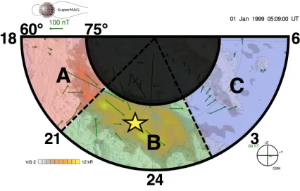
Figure 1. SuperMAG polar plot indicating the spatial regions A, B and C for which we
ob-tain sub-networks. All data is from stations between 60 − 75◦magnetic latitude, within the nightside. The LT boundaries between A, B and C are different for each event and are
deter-mined from Polar VIS images; they are separated by the east and west boundaries of the bulge
at the time of maximum expansion (dashed lines). The magnetic latitude and local time of onset
(again from Polar VIS) for each event, are indicated by the yellow star.
206 207 208 209 210 211
aries of the bulge fifteen normalized minutes before, and after, the maximum expansion
220
phase (t0 = 15 and t0 = 45), results are presented in the SI. This gives slight
differ-221
ences but the overall results and conclusions are unchanged. The SCW is typically six
222
hours of local time in extent (Gjerloev et al., 2007) which corresponds to region B;
re-223
gions A and C are westwards and eastwards of the SCW respectively.
224
We will present a detailed study of the sub-networks for a single event and then
225
will compare it to the average sub-network behaviour seen across all 86 isolated substorms.
226
An event was identified which has≥7 magnetometer stations in each of regions A, B
227
and C for the duration of the substorm; this occurs on 01−Jan−1999 with onset at 04 :
228
52 UT. It had a relatively short expansion phase, 17 minutes, and a thin SCW,
extend-229
ing over 4.1 hours of LT at the time of peak expansion (t0= 30). For the averaged study
230
over 86 events we require at least three magnetometers in a spatial region for it’s
sub-231
network to be included in the study. For example, a substorm in which there were≥3
232
magnetometers in regions A and B, but< 3 in C, will contribute to the average
sub-233
networks behaviour within A and B but not within sub-network C. We repeated the
en-234
tire analysis with the more restrictive criterion of≥7 magnetometers and found very
235
similar results (see SI). One benefit of using network analysis is that we do not require
236
a spatially uniform grid of magnetometers, that being said, the condition of having≥
237
3 magnetometers per region gives a mean spatial separation distance (within regions)
238
of∼1000km.
239
The spatial regions A, B and C are defined such that the sub-networks are always
240
in the same local time relative to the SCW but, as the earth rotates, the geomagnetic
241
location of the magnetometer stations will vary. This will not affect the properties of the
242
computed network provided regions A, B, C continue to be well-sampled with stations.
243
However, the number of stations within each region can change. We therefore include
244
a normalization to the number of possible connections to define the parameter that we
245
will use to quantify the network, the normalized number of connections:
246
α(t) = PN(t)
i6=j
PN(t)
j6=i Aij
N(t)(N(t)−1) (2) whereAis the adjacency matrix andN(t) is the number of active magnetometers.
4 Results
248
200 400 600
SME (nT)
01-Jan-1999
200 400 600
SME (nT)
Mean (86 Substorms)
0 0.5 1
0 0.5
0 0.5 1
0 0.5
0 0.5 1
0 0.5
Onset Peak
0 0.5
0 0.2
0 0.5
0 0.2
0 0.5
0 0.2
0 0.5
0 0.2
0 0.5
0 0.2
-10 0 10 20 30 40 50
Normalized time, t (mins ) 0
0.5
-10 0 10 20 30 40 50
Normalized time, t (mins ) 0
0.2
0 5 10 15
[image:8.612.92.488.72.614.2]| c
| (mins)
5) A B
6) B A
7) A C
8) C A
10) C B 9) B C 4) C 3) B 2) A
5) A B
6) B A
7) A C
8) C A
9) B C 2) A
3) B
4) C
1) 1)
10) C B
Figure 2. The normalized number of connections,α(t0, τc), is binned by the lag of
maxi-mal canonical cross-correlation (CCC),|τc|. Each panel stacks vertically (one above the other) α(t0, τc) versus normalized time,t0, for|τc| ≤ 15. |τc|is indicated by colour (see colour bar).
Panel 1 plots the SuperMAG electrojet index, SME. Panels 2 − 10 plotαfor connections within and between each of the regions A, B and C (identified in Figure 1). The left columns plot a
single event, whereas the right plots the average of 86 events (containing sub-networks with≥ 3 magnetometers per region). Substorm onset (green dashed line) is att0 = 0 and the maximum of
the expansion phase (purple dashed line) is att0= 30.
4.1 Observed timings of spatial correlation
257
We now present (in figure 2) the directed network for the individual substorm
iden-258
tified above (left column), and the average of all 86 selected substorms (right column).
259
Substorm evolution is not necessarily linear but the individual substorm is plotted as an
260
example to highlight that the multi-event mean is a reasonable average. Having obtained
261
the sub-networks for each region (identified in figure 1), we have the normalized
num-262
ber of connections,α(t0, τc) (equation 2) within (panels 2−4), or between the regions
263
A, B and C (panels 5−10). Looking at connected magnetometers within each region
264
provides timings of the emergence of coherent spatial patterns of correlation in the
mag-265
netic field perturbations (at ground level), whilst connections between regions provide
266
information on how these patterns are propagating and/or expanding through out the
267
substorm; any inter-region dependencies will also be flagged. If all possible
magnetome-268
ter connections are present thenα= 1. Since the connections between regions (e.g. A→C
269
and C→A) are plotted separately (e.g. panel 7 and 8), then if these were fully connected,
270
the sum over the two plots would be 1. Hence the range of values for the y-axes for
con-271
nections between regions (panels 5-10) are half the size of that within the regions
(pan-272
els 2-4).
273
As the networks are constructed using the time delay/lag at which the CCC
be-274
tween each pair of magnetometer stations is maximal, each connection has an associated
275
signed lag,τc. We bin the number of connections (α) into ranges of the magnitude of
276
this lag (τc). Connections which are at zero lag have no time delay i.e. τc = 0 (grey),
277
and connections with an associated direction of propagation/ expansion, from one
mag-278
netometer to another, have a range of delays, that is, lags from 1−15 minutes
(blue-279
red). The sign of the lag indicates a direction of propagation or expansion from one
mag-280
netometer location to another; this information is combined with the physical
geograph-281
ical locations of the magnetometers to determine if the propagation/expansion is
east-282
ward or westward. The connections are separated into different panels for each
direc-283
tion and then binned by the magnitude of the lag. For example, between regions A and
284
C, panel 7 plots the A→C propagation/expansion, eastward, from region A into region
285
C whilst panel 8 plots C→A propagation/expansion, westward, from region C into
re-286
gion A. Connections with a lagτc = 0 (indicated in grey) are plotted on both panels
287
7 and 8 (A→C and C→A) as they simply indicate instantaneous correlation between
re-288
gions A and C, which have no associated direction and thus, by definition the grey bars
289
are identical on the two plots.
290
Figure 2 stacks the time series of the normalized number of connections,α(t0, τc),
291
so that the value ofαfor each range of |τc|are plotted one above the other for
increas-292
ing|τc|. The stacking is such that each independentα(t0, τc) is visible. The envelope
293
is then the total (normalized) number of connections over all lags, that is, all| τc |≤
294
15. For example, during the individual substorm (left column), we see mostly
instanta-295
neous (grey) correlation within A (panel 2) with an additional low level of lagged
cor-296
relation later in the substorm. On the other hand within B (panel 3), at the time of peak
297
expansion (purple dashed line) the network is made up of∼10% instantaneous
corre-298
lation,∼ 80% with 1 ≤| τc |≤ 5 (fast propagating or expanding) and< 10% of
con-299
nections have| τc |≥6 (slow expansion or propagation). The plot covers the time
in-300
terval−10 ≤ t0 ≤ 50 normalized minutes where the times of onset, peak expansion
301
and the 10 minute intervals in-between are indicated with vertical dashed lines. The
fig-302
ure presents a summary of time-varying spatial correlation for each sub-network for the
303
duration of the substorm. The full networks for the individual substorm are plotted in
304
the SI. The SME (SuperMAG electrojet index) for the individual event, and its
multi-305
event average, is plotted in panel 1 of figure 2. We can see that although the events are
306
on a normalized time-base, the multi-event average is more smooth and responds less
307
sharply to onset than the individual event.
Prior to onset, the multi-event average shows some spatially coherent connections
309
within each of regions A and C (panels 2 and 4). These connections are mostly
instan-310
taneous (| τc |= 0, grey shading) or with 1 minute lag (| τc |= 1, dark blue shading).
311
Importantly these regions are not correlated with each other, so that the number of A→C
312
and C→A connections are small (panels 7 and 8). At onset, in both the individual event
313
and the statistical average, (panel 3) we see that the sub-network within region B has
314
the most prompt and largest response, that is, increase in spatial correlation. For the
315
individual substorm we see a sharp increase in the number of correlated pairs, beginning
316
at onset (t0 = 0) and increasing to∼100% (all magnetometers within B are highly
cor-317
related) att0∼15. Likewise, the multi-event average number of correlated
magnetome-318
ter pairs within the B sub-network begins to increase at onset, but it is smoother and
319
reaches a peak slightly later than in the individual event; in this case, correlation
max-320
imizes with∼60% connectivity att0∼25. The January substorm onset is mainly
char-321
acterized by fast propagating (0−6 minutes lag) connections whilst in the multi-event
322
mean sub-network∼80% of connections are propagating (non-zero peak lag)
through-323
out. This is consistent with a pattern that is both coherent and propagating and/or
ex-324
panding. The timings of region B growth are consistent across the majority of substorms
325
observed.
326
About 10 normalized minutes after onset we can see in panel 6 westward
propa-327
gation and/or expansion from region B (around onset) into region A (westward of
on-328
set), B→A. This coincides with an increase in spatial correlation within region A (panel
329
2). For both the individual and the multi-event average, the B→A time series (panel 6),
330
that is, the relative increase in the number of connections at different lags, resembles that
331
of the network located wholly within region B (panel 3), except that it occurs∼10
nor-332
malized minutes later and has about half the magnitude. Within region A (panel 2),∼
333
50% of magnetometers become highly correlated at 20 < t0 < 30. For the individual
334
substorm most of the connections between magnetometers are instantaneous, but for the
335
multi-event average∼ 2
3 of the increase in the number of connections is at non-zero lag.
336
We have found some variation between individual substorms as to how spatial
correla-337
tion between magnetometers within region A develops from−10≤t0≤50, with some
338
substorms having no obvious response to onset. The A→B (panel 5) propagation and/or
339
expansion develops on similar timescales to B→A (panel 6) but there are significantly
340
fewer connections (20−30% of magnetometers correlated at peak,t0= 30) within the
341
multi-event average, with∼ 1
3 of these connections being instantaneous (zero lag, no
342
direction).
343
The sub-network for region C (panel 4, east of the SCW) has the smallest response
344
to substorm onset of any region. The January substorm remains moderately connected
345
(∼23%) from before onset until long after peak expansion. The multi-event average
be-346
gins to increase at 10< t0 <20 and the region is maximally correlated after peak
ex-347
pansion,t0 > 30 with∼ 20% of magnetometer pairs being connected; this pattern of
348
correlation is consistent long into the recovery phase. This is consistent with many of
349
the individual substorms showing little/no response to onset. In panel 9 we see that
re-350
gion B becomes correlated with region C with eastwards propagation and/or expansion
351
(B→C)∼10−20 normalized minutes after onset, peaking with∼20% magnetometer
352
pairs correlated att0>30. In panel 10, we can see that for the individual event <10%
353
of magnetometers are correlated from C→B, with this small increase only occurring∼
354
25 normalized minutes after onset. Correlation increases by∼15% for the multi-event
355
average betweent0 ∼10 andt0∼30. Thus the response within region C simply tracks
356
that of the propagation or expansion from B→C, and any propagation from C→B
357
occurs subsequently.
358
Finally,∼10−20 normalized minutes after onset, in panels 7 and 8 we see
cor-359
relation growing relatively slowly between regions A and C (west and east of the onset
360
location, respectively), reaching a maximum level of connectedness att0∼40, long
ter the time of peak expansion. There is slightly more eastward propagation (A→C,>
362
20% of magnetometers) than westward propagation (C→A,∼10% and∼18% of
mag-363
netometer pairs for the individual and multi-event average, respectively). Again, the lagged
364
correlation originating in C is very small (and mostly instantaneous) for the individual
365
event.
366
4.2 Interpretation
367
If we can interpret coherent patterns of spatial correlation across the distributed
368
SuperMAG magnetometers as the emergence of current systems, the above time-dependent
369
network provides an evolution sequence, with timings, for the substorm current system
370
in the nightside. Our analysis then provides a quantitative measure of spatial coherence
371
as well as the time scales on which evolution occurs. By separating the nightside into
372
three regions we have attempted to isolate the components that have been proposed. To
373
use the terminology of Kamide and Kokubun (1996) we have: (A) eastward electrojet;
374
(B) substorm unloading component (SCW) and (C) westward electrojet. Whereas B is
375
associated with the substorm current wedge, or DP1 perturbations, A and C can be
re-376
lated to the general magnetospheric convective system, DP2 (Nishida, 1968), which is
377
enhanced during substorm growth and expansion phases (Milan et al., 2017). To
sum-378
marize the above results we identify key time ranges, before and after onset: 0≤t01<
379
10, 10≤t02 <20, 20 ≤t30 <30 andt04 ≥30 in terms of normalized time,t0. Relating
380
these intervals to substorm evolutiont01 is following onset,t02 is expansion phase,t03 is
381
near substorm peak andt04 is the early recovery phase. The timings are:
382
• Before onset, the pre- and post-midnight regions A and C each have a relatively
383
weak coherent pattern consistent with convection (DP2); notably A and C are not
384
coherent with each other.
385
• Int0
1we first see the formation of a substorm current wedge (SCW/DP1) around
386
onset (correlation within B) which approaches maximum int02.
387
• Int0
2there is westward propagation and/or expansion of the SCW west towards
388
the pre-midnight region (A). We see connections (B→A) and at the same time a
389
signature of a coherent current system within region A (correlation within A). This
390
is shortly followed by weaker correlation from A→B, indicating that the entire
A-391
B system is now correlated. These all approach a maximum att03.
392
• A weaker signal of eastward propagation and/or expansion of the SCW towards
393
the post-midnight region starts int02, and reaches its maximum int04. We see
con-394
nections (B→C) and on a similar timescale a signature of a coherent current
sys-395
tem within region C (correlation within C), with additional weaker correlation from
396
C→B. The correlation in region C is relatively low.
397
• The regions eastward and westward of onset (A and C) each have a coherent
pat-398
tern consistent with enhanced magnetospheric convection (DP2). Later in the
sub-399
storm there is coherence between regions A and C, beginning well after onset, in
400
t02, and reaching maximum correlation int04, that is, only after region B has
be-401
come correlated with all other regions. This can either reflect direct correlation
402
between A and C, or could simply imply that both A and C are correlated with
403
B.
404
We can then consider what support these results provide for proposed models for
405
substorm current systems, specifically, models with a single westward electrojet segment
406
(Kamide & Kokubun, 1996; McPherron et al., 1973), a westward and, a lower (but still
407
in the auroral zones) latitude eastward electrojet segment (Ritter & L¨uhr, 2008; Sergeev
408
et al., 2014, 2011); two unconnected westward electrojet segments pre- and post-midnight
409
(Gjerloev & Hoffman, 2014; Rostoker, 1996) and finally many small individual segments
410
(Liu et al., 2018). Importantly, any method for quantifying spatial correlation cannot
411
distinguish between direct correlation (here, A→C) and indirect correlation (here, A→B→C);
this indirect correlation may enhance the number of A→C connections relative to B→C.
413
Therefore our results are not inconsistent with multiple separate current systems
pro-414
vided that they are either spatially correlated with each other, or on spatial scales smaller
415
than that of the magnetometer spacing.
416
The coherent patterns of eastward and westward expansion are in agreement with
417
previous work using synchronous space and ground based magnetometers (Nagai, 1982,
418
1991). However, we have not found definitive support for two, or more, distinct and
un-419
correlated substorm current systems. A lag,| τc |> 0, for B→C connections, implies
420
that C is delayed with respect to B, consistent with a propagation from B to C.
Inter-421
preting these results in terms of current components suggest two scenarios for this
prop-422
agation: i) a single current segment which is expanding from B to C; or, ii) a current
seg-423
ment in B and another in C, where the segment in C is correlated with that in B but
424
is developing with some delay. There is no interpretation of our results which would
sug-425
gest a scenario where regions B and C are uncorrelated, independent current systems.
426
If they are associated entirely with general magnetospheric convection (DP2
sys-427
tem), the pre- and post- midnight (A and C) are directly-driven by the solar wind and
428
must enhance on similar time-scales, although the magnitudes may differ (Kamide & Kokubun,
429
1996). We have found that pre-onset, the regions A and C each have coherent, but
rel-430
atively small, signatures of correlation with little CCC between them. Post-onset, in both
431
the individual event and the average over 86 substorms, the long range east to west (A→C)
432
correlation patterns only emerge after the growth of the SCW (region B). The growth
433
of spatially coherent patterns appears first in B (the SCW, at onset) followed by A (with
434
correlation between B and A) and later, in C. This suggests that following onset, A and
435
C are not solely attributable to enhanced convection and the presence of
contempora-436
neous B→C and B→A connections suggests that there may be a combination of
con-437
tributions from convection enhancement and SCW expansion. Importantly, this does not
438
require that a current segment in A expands or propagates into C.
439
Finally, if instead of a large scale SCW there were only many small, uncorrelated,
440
individual segments (Liu et al., 2018) we would not expect to find the long-range
cor-441
relations (A to C) seen here (also SI, figure 1). Since we calculate CCC on minute
res-442
olution time series, each connection in the network is derived from a 128 minute time
443
window. Thus we cannot resolve short-timescale events such as a large number of small
444
wedgelets each associated with a bursty bulk flow (BBF) in the plasma sheet which have
445
lifetimes of some 10 min. In addition, we cannot resolve structures that are on smaller
446
spatial scales than the inter-magnetometer spacing. If multiple wedgelets are present,
447
their spatial aggregate would give an overall large-scale magnetic amplitude signature
448
mainly at the edges of the region containing the wedgelets, regardless of whether or not
449
the wedglets are spatio-temporally correlated. Here, both spatial and temporal
informa-450
tion is used to obtain the cross-correlation so that temporally uncorrelated wedgelets would
451
give no spatially coherent signature of cross correlation at all, whereas if the same wedgelets
452
were temporally correlated, we would find a signature of spatial cross-correlation.
453
Potential limitations to the technique include sensitivity to the location of the east
454
and west bulge boundaries, which are static and therefore may not fully represent fast
455
changes in the time-varying current system. There may also be a spatial coarse-graining
456
effect due to the geographic location of the finite number of magnetometers; there are
457
few near the eastward SWC boundary during the January substorm. To test this we present
458
the same plots for this event, but with the east and west boundaries of the bulge att0 =
459
15 andt0 = 45 in the SI. These show little change from the results shown in Figure 2.
460
Additionally, the detailed network maps of the individual event, for the times represented
461
by the vertical dashed lines in Figure 2, onset-peak, are provided in the SI. They
high-462
light the importance of the spatial coverage and geographical locations of the highly
cor-463
related magnetometer pairs.
Also, in the analysis and by the organization of data into three regions, A, B, C,
465
we are quantifying the coherence over these regions. This is over a range in both
lati-466
tude (60−75◦) and local time (typically region B is ∼6 hrs LT). The westward
elec-467
trojet around onset (B) may not cover all latitudes but our analysis technique is mainly
468
addressing the various SCW models which differ in their local time distribution.
469
5 Conclusions
470
We used the full set of SuperMAG ground-based magnetometer observations of
iso-471
lated substorms to quantify the time evolution of patterns of spatial correlation. If the
472
observed pattern of spatial correlation between magnetometer observations captures
iono-473
spheric current patterns then we can directly test different models for substorm
iono-474
spheric current systems. We have obtained the first directed networks for isolated
sub-475
storms. Each connection in the network indicates when the maximum canonical
cross-476
correlation CCC between the vector magnetic field perturbations seen at each pair of
mag-477
netometers exceeds an event and station specific threshold. The maximum of the CCC
478
corresponding to each connection in the network can occur at a non-zero time lag. The
479
resultingdirected network then contains information, not only on the formation of
co-480
herent patterns seen by multiple magnetometers, but also on the propagation and/or
ex-481
pansion of these spatially coherent structures.
482
To gain insight on the ionospheric current system during a substorm, we obtained
483
specific time-varying sub-networks from the data which isolate specific physical regions.
484
These regions are west (A), within (B) and east (C) of the bulge boundaries for each
sub-485
storm (obtained from polar VIS images at the time of peak expansion). We presented
486
both a study of an individual event, which has at least seven magnetometers in each of
487
these regions for the duration of the substorm, as well as the average of the network
prop-488
erties of 86 substorm events. If the observed pattern of spatial correlation between
mag-489
netometer observations captures ionospheric current patterns, we find the following
se-490
quence of events in terms of key time ranges after onset: 0 ≤t01 <10, 10 ≤ t02 < 20,
491
20≤t03<30 andt04≥30 (t0 is normalized time (Gjerloev et al., 2007)):
492
• Pre- onset, the pre- and post-midnight regions A and C each have a relatively weak
493
coherent pattern consistent with general magnetospheric convection (DP2) and
494
are not coherent with each other.
495
• A dominant substorm current wedge (SCW) forming around the onset location
496
(within region B) at the time of onset,t1, which reaches maximum spatial
corre-497
lation att2, half way through the expansion phase.
498
• This is followed by a westward expansion of this SCW (starting att2, with peak
499
att3) contemporaneous to and coherent with a current system in the pre-midnight
500
region (within A).
501
• An additional weaker eastward expansion of the SCW (starting slowly att2 with
502
peak att4). The signal of a self-contained current post-midnight (region C) is
rel-503
atively weaker and occurs late in the substorm. The enhancement of C is delayed
504
with respect to that of A.
505
• Following the SCW expansion, A and C are coherent with each other, but at the
506
same time are coherent with the SCW. This is consistent with a combination of
507
convection and expansion of the SCW.
508
These conclusions are drawn from the averaged network over 86 isolated substorms.
509
Although the overall spatio-temporal timings revealed by this network analysis are
rea-510
sonably consistent between individual events and the 86 event average for the formation
511
of a SCW around onset (B) and it’s expansion both east (B→C) and west (B→A), the
512
exact timings of the current system evolution varies. Variability between events could
513
be intrinsic or could relate to the observing conditions, such as differing magnetometer
spatial coverage or the static choice of location for region boundaries. Future work will
515
quantify event-by-event variability across multiple events and extend the analysis to
mul-516
tiple, compound events. So far in our analysis we have not utilized the direction of the
517
(vector) maximal CCC. In principle this could resolve the direction of the electojet
(east-518
ward/westward).
519
Acknowledgments
520
We acknowledge use of the SuperMAG ground magnetometer station data fromhttp://
521
supermag.jhuapl.edu/and thank Rob Barnes for providing us with a hard copy (Dec
522
2017). S. C. C acknowledges a Fulbright-Lloyds of London Scholarship, AFOSR grant
523
FA9550-17-1-0054 and STFC ST/P000320/1. We thank the Santa Fe Institute for
host-524
ing a visit during which we worked on this research.
525
References
526
Akasofu, S.-I. (1964). The development of the auroral substorm. Planetary and
527
Space Science,12(4), 273–282.
528
Albert, R., & Barab´asi, A.-L. (2002). Statistical mechanics of complex networks.
Re-529
views of modern physics,74(1), 47.
530
Boccaletti, S., Latora, V., Moreno, Y., Chavez, M., & Hwang, D.-U. (2006).
Com-531
plex networks: Structure and dynamics. Physics reports,424(4-5), 175–308.
532
Dods, J., Chapman, S., & Gjerloev, J. (2015). Network analysis of geomagnetic
sub-533
storms using the supermag database of ground-based magnetometer stations.
534
Journal of Geophysical Research: Space Physics,120(9), 7774–7784.
535
Dods, J., Chapman, S., & Gjerloev, J. (2017). Characterizing the ionospheric
536
current pattern response to southward and northward imf turnings with
dy-537
namical supermag correlation networks. Journal of Geophysical Research:
538
Space Physics,122(2), 1883–1902.
539
Gjerloev, J. (2012). The supermag data processing technique. Journal of
Geophysi-540
cal Research: Space Physics,117(A9).
541
Gjerloev, J., & Hoffman, R. (2014). The large-scale current system during
auro-542
ral substorms. Journal of Geophysical Research: Space Physics,119(6), 4591–
543
4606.
544
Gjerloev, J., Hoffman, R., Sigwarth, J., & Frank, L. (2007). Statistical description
545
of the bulge-type auroral substorm in the far ultraviolet. Journal of
Geophysi-546
cal Research: Space Physics,112(A7).
547
Jost, J. (2007). Dynamical networks. InNetworks: from biology to theory (pp. 35–
548
62). Springer.
549
Kamide, Y., & Kokubun, S. (1996). Two-component auroral electrojet:
Impor-550
tance for substorm studies. Journal of Geophysical Research: Space Physics,
551
101(A6), 13027–13046.
552
Kullen, A., & Karlsson, T. (2004). On the relation between solar wind,
pseudo-553
breakups, and substorms. Journal of Geophysical Research: Space Physics,
554
109(A12).
555
Liu, J., Angelopoulos, V., Yao, Z., Chu, X., Zhou, X.-Z., & Runov, A. (2018). The
556
current system of dipolarizing flux bundles and their role as wedgelets in the
557
substorm current wedge. Electric Currents in Geospace and Beyond, 323–337.
558
Malik, N., Bookhagen, B., Marwan, N., & Kurths, J. (2012). Analysis of spatial and
559
temporal extreme monsoonal rainfall over south asia using complex networks.
560
Climate dynamics,39(3-4), 971–987.
561
McGranaghan, R. M., Mannucci, A. J., Verkhoglyadova, O., & Malik, N. (2017).
562
Finding multiscale connectivity in our geospace observational system: Network
563
analysis of total electron content. Journal of Geophysical Research: Space
564
Physics,122(7), 7683–7697.
McPherron, R. L., Russell, C. T., & Aubry, M. P. (1973). Satellite studies of
mag-566
netospheric substorms on august 15, 1968: 9. phenomenological model for
567
substorms. Journal of Geophysical Research,78(16), 3131–3149.
568
Milan, S. E., Clausen, L. B. N., Coxon, J. C., Carter, J. A., Walach, M.-T., Laundal,
569
K., . . . others (2017). Overview of solar wind–magnetosphere–ionosphere–
570
atmosphere coupling and the generation of magnetospheric currents. Space
571
Science Reviews,206(1-4), 547–573.
572
Nagai, T. (1982). Observed magnetic substorm signatures at synchronous altitude.
573
Journal of Geophysical Research: Space Physics,87(A6), 4405–4417.
574
Nagai, T. (1991). An empirical model of substorm-related magnetic field variations
575
at synchronous orbit. Washington DC American Geophysical Union
Geophysi-576
cal Monograph Series, 64, 91–95.
577
Newman, M. E. (2003). The structure and function of complex networks. SIAM
re-578
view,45(2), 167–256.
579
Nishida, A. (1968). Coherence of geomagnetic dp 2 fluctuations with interplanetary
580
magnetic variations. Journal of Geophysical Research,73(17), 5549–5559.
581
Pulkkinen, A. (2015). Geomagnetically induced currents modeling and forecasting.
582
Space Weather, 13(11), 734–736.
583
Reinsel, G. C. (2003). Review of canonical correlations in multivariate analysis.
584
InElements of multivariate time series (p. 68-70). Springer Science & Business
585
Media.
586
Richmond, A., & Kamide, Y. (1988). Mapping electrodynamic features of the
587
high-latitude ionosphere from localized observations: Technique. Journal of
588
Geophysical Research: Space Physics,93(A6), 5741–5759.
589
Ritter, P., & L¨uhr, H. (2008). Near-earth magnetic signature of magnetospheric
590
substorms and an improved substorm current model. InAnnales geophysicae
591
(Vol. 26, pp. 2781–2793).
592
Rostoker, G. (1996). Phenomenology and physics of magnetospheric substorms.
593
Journal of Geophysical Research: Space Physics,101(A6), 12955–12973.
594
Sergeev, V., Nikolaev, A., Tsyganenko, N., Angelopoulos, V., Runov, A., Singer, H.,
595
& Yang, J. (2014). Testing a two-loop pattern of the substorm current wedge
596
(scw2l). Journal of Geophysical Research: Space Physics,119(2), 947–963.
597
Sergeev, V., Tsyganenko, N., Smirnov, M., Nikolaev, A., Singer, H., & Baumjohann,
598
W. (2011). Magnetic effects of the substorm current wedge in a spread-out
599
wire model and their comparison with ground, geosynchronous, and tail lobe
600
data. Journal of Geophysical Research: Space Physics,116(A7).
601
Stolbova, V., Tupikina, L., Bookhagen, B., Marwan, N., & Kurths, J. (2014).
Topol-602
ogy and seasonal evolution of the network of extreme precipitation over the
603
indian subcontinent and sri lanka. Nonlinear Processes in Geophysics.
604
Tanskanen, E., Pulkkinen, T., Koskinen, H., & Slavin, J. (2002). Substorm energy
605
budget during low and high solar activity: 1997 and 1999 compared. Journal
606
of Geophysical Research: Space Physics,107(A6).
607
Watts, D. J., & Strogatz, S. H. (1998). Collective dynamics of small-worldnetworks.
608
nature,393(6684), 440.
609
Wiedermann, M., Radebach, A., Donges, J. F., Kurths, J., & Donner, R. V. (2016).
610
A climate network-based index to discriminate different types of el ni˜no and la
611
ni˜na. Geophysical Research Letters,43(13), 7176–7185.