Patron: Her Majesty The Queen Rothamsted Research Harpenden, Herts, AL5 2JQ
Telephone: +44 (0)1582 763133 Web: http://www.rothamsted.ac.uk/
Rothamsted Research is a Company Limited by Guarantee Registered Office: as above. Registered in England No. 2393175. Registered Charity No. 802038. VAT No. 197 4201 51. Founded in 1843 by John Bennet Lawes.
Rothamsted Repository Download
A - Papers appearing in refereed journals
Bock, C. H., Gottwald, T. R., Parker, P. E., Ferrandino, F., Welham, S. J.,
Van Den Bosch, F. and Parnell, S. 2010. Some consequences of using
the Horsfall-Barratt scale for hypothesis testing. Phytopathology. 100
(10), pp. 1030-1041.
The publisher's version can be accessed at:
•
https://dx.doi.org/10.1094/PHYTO-08-09-0220
The output can be accessed at:
https://repository.rothamsted.ac.uk/item/8q6q6/some-consequences-of-using-the-horsfall-barratt-scale-for-hypothesis-testing
.
© Please contact [email protected] for copyright queries.
Analytical and Theoretical Plant Pathology
Some Consequences of Using the Horsfall-Barratt Scale
for Hypothesis Testing
C. H. Bock, T. R. Gottwald, P. E. Parker, F. Ferrandino, S. Welham, F. van den Bosch, and S. Parnell
First author: United States Department of Agriculture (USDA) Agricultural Research Service (ARS)–SEFTNRL, 21 Dunbar Rd., Byron, GA 31008; second author: USDA ARS–USHRL, 2001 S. Rock Rd., Ft. Pierce, FL 34945; third author: USDA Animal and Plant Health Inspection Service–PPQ, Moore Air Base, Edinburg, TX 78539; fourth author: Department of Plant Pathology and Ecology, Connecticut Agricultural Experiment Station, New Haven 06511; and fifth, sixth, and seventh authors: Rothamsted Research, Harpenden, Herts., AL5 2JQ, England, UK.
Accepted for publication 4 June 2010.
ABSTRACT
Bock, C. H., Gottwald, T. R., Parker, P. E., Ferrandino, F., Welham, S., van den Bosch, F., and Parnell, S. 2010. Some consequences of using the Horsfall-Barratt scale for hypothesis testing. Phytopathology 100:1030-1041.
Comparing treatment effects by hypothesis testing is a common practice in plant pathology. Nearest percent estimates (NPEs) of disease severity were compared with Horsfall-Barratt (H-B) scale data to explore whether there was an effect of assessment method on hypothesis testing. A simulation model based on field-collected data using leaves with disease severity of 0 to 60% was used; the relationship between NPEs and actual severity was linear, a hyperbolic function described the relationship between the standard deviation of the rater mean NPE and actual disease, and a lognormal distribution was assumed to describe the frequency of NPEs of specific actual disease severities by raters. Results of the simulation showed standard deviations of mean NPEs were consistently similar to the original rater standard deviation from the field-collected data; however, the standard deviations of the H-B scale data deviated from that of the original rater standard deviation, particularly at 20 to 50% severity, over which H-B scale grade intervals are widest; thus, it is over this range that differences in hypothesis testing are most likely to
occur. To explore this, two normally distributed, hypothetical severity populations were compared using a t test with NPEs and H-B midpoint data. NPE data had a higher probability to reject the null hypothesis (H0) when H0 was false but greater sample size increased the probability to reject H0 for both methods, with the H-B scale data requiring up to a 50% greater sample size to attain the same probability to reject the H0 as NPEs when H0 was false. The increase in sample size resolves the increased sample variance caused by inaccurate individual estimates due to H-B scale midpoint scaling. As expected, various population characteristics influenced the probability to reject H0, including the difference between the two severity distribution means, their variability, and the ability of the raters. Inaccurate raters showed a similar probability to reject H0 when H0 was false using either assessment method but average and accurate raters had a greater probability to reject H0 when H0 was false using NPEs compared with H-B scale data. Accurate raters had, on average, better resolving power for estimating disease compared with that offered by the H-B scale and, therefore, the resulting sample variability was more representative of the population when sample size was limiting. Thus, there are various circumstances under which H-B scale data has a greater risk of failing to reject H0 when H0 is false (a type II error) compared with NPEs.
Plant disease severity—the proportion of a plant unit diseased (31)—can be assessed in various ways. There are several kinds of disease assessment scales that have been developed to help estimate the amount of disease on a leaf or plant or in a plot or field (2,7,23). One of the most widely used scales in plant disease assessment is the Horsfall-Barratt (H-B) scale (15) and its plethora of offspring; however, its characteristics and the ramifi-cations of using the scale have only recently begun to be explored (2,10,12,25,26).
The H-B scale (15) divides the percent scale into 12 logarith-mic-based severity intervals between 0 and 100%. The interval sizes are symmetrical either side of 50% (Table 1), with the symmetry being based on the (apparently unproven) observation that the eye reads diseased tissue at <50% disease and healthy tissue at >50% disease (15).
Disease severity assessments are often made using the H-B scale. The original article (15) has been cited at least 561 times (39), and Current Contents (14) interviewed Horsfall on the
original Horsfall and Barratt article (15) under the “Citation Classics” feature. Originally, Horsfall and Barratt (15) and Horsfall (13) recommended averaging the grade values prior to using a calibration curve to read actual disease on the y-axis (a process that removed heterogeneity of variance, because each grade is given equal weight) but this resulted in bias (34). Thus, the requirement to convert each grade measurement back to a percentage (thereby reasserting heterogeneity of variance) was necessary. The process for converting the H-B scale estimates into a mean severity is as follows: first, the appropriate grade on the scale is allotted to each individual in a sample of leaves or plants (15); second, for each grade, the percent range midpoint is taken directly or using the Elanco conversions (34); and third, the percent midpoints for all individuals in the sample are summed and averaged (sum of midpoint percents/sample size) to arrive at the estimated mean percent disease severity.
The use of the H-B-scale has been the subject of controversy for almost as long as it has been around (1,2,7,9–12,18,25,26). The interpretation that the scale described an apparent logarithmic relationship between estimated and actual disease severity has now been shown not to be the case (3,5,12,25,26,29). A linear relationship exists between estimated disease and actual disease. However, the nature of the relationship between the variance (or standard deviation, or estimation error) and the magnitude of the actual value has not been fully established. Nonconstancy of
Corresponding author: C. H. Bock; E-mail address: [email protected]
doi:10.1094 / PHYTO-08-09-0220
variance with magnitude of actual disease is widely reported (2,4, 9–11) and individuals vary greatly in their ability to assess dis-ease; therefore inter- and intra-rater reliability is a further source of error in assessments (2,3,11,25,29). Furthermore, Hau et al. (11) demonstrated that characteristics of the distribution of dis-eased leaves in the population and the number of classes in a disease scale affected the accuracy of the estimate of mean disease severity. Very skewed populations rated using a scale with few grades (<7) resulted in inaccurate mean estimates, although they did not compare these interval-scale estimates to nearest percent estimates (NPEs) or investigate the effects of sample size. There is also evidence that estimates of disease severity based on the H-B scale are most often less precise (sensu Madden et al. for measurement agreement [23]) compared with NPEs (2,25).
Testing for treatment differences is a standard procedure in plant pathology. In many cases, two treatments (e.g., disease control options) are applied to plants in different plots, the severity of the disease subsequently estimated, and the resulting data sets analyzed. The statistical analysis often aims at testing the null hypothesis (H0) that the mean disease severities in the two
treatments are equal. Rejecting the H0 is then used as indication
that the two treatments actually have different effects on the severity of disease or the development of the epidemic (6,8,24, 32,33). A standard way to test for differences in mean disease severity on a continuous scale such as percent disease severity is by using a t test (37). In the case of data generated using the H-B scale, the test uses the percent range midpoints of the grade assigned to each observation in the two data sets. Alternatively, using the grade numbers, a nonparametric test, of which the Mann-Whitney U test is an example, could be used to compare medians of the treatments. The Mann-Whitney U test is suffici-ently analogous to the t test to serve as a comparison and does not require the assumption of continuous data.
It has not been demonstrated how the use of the H-B scale affects hypothesis testing. Exploring the effects of H-B scaled data on hypothesis testing is the main objective of this study. Is use of the H-B scale less or more likely to (correctly) reject the H0
when there actually is a difference between the mean severities in the two treatments, compared with NPEs of disease severity? NPEs of disease severity are notoriously variable (5,25,28), reducing the probability to reject the H0 when there actually is a
difference between the mean severities in the two treatments (32). On the other hand, using the H-B scale and midpoint values might introduce additional variability into the samples (2,10,25). The effect of H-B scaled data on the probability to reject H0 when H0
is false has not been explored.
To explore the effects of using the H-B scale on hypothesis testing, we developed a generalized rater estimation distribution, based on a previous data set (3,4). We used this model in a simulation study to sample from two hypothetical disease severity distributions, using both the H-B scale and NPEs. The samples from the disease severity distributions were analyzed using the t
test (NPE and H-B midpoint data) and the Mann-Whitney U test (grade data) to compare the probability to reject H0.
THEORY AND APPROACHES
Actual and estimated disease severity. The data described by Bock et al. (3,4) were used to develop a model that describes a generalized rater ability to estimate disease at different severities of 0 to 60%. The original data were based on a sample of 210 citrus canker (Xanthomonas citri subsp. citri)-infected grapefruit leaves and encompass (i) measurements of the “actual” disease severity on a leaf-by-leaf basis using image analysis (ASSESS; American Phytopathological Society, St. Paul, MN) and (ii) rater NPEs of disease severities for each of the 200 leaves on two separate occasions.
Combining the NPEs of the three raters from two separate assessment occasions was assumed to provide an adequate description of generalized distribution characteristics of estimates of specific actual disease severities over that disease range.
To achieve sufficient data to estimate the mean and standard deviation at different actual disease severities, the data were grouped in actual severity intervals of 0 to 1, 1+ to 2, 2+ to 3, 3+ to
5, 5+ to 7.5, 7.5+ to 10, 10+ to 15, 15+ to 20, 20+ to 30, 30+ to 40,
and 40+ to 60% disease. To describe the mean rater estimated
severity, µrater, as a function of the actual severity, µactual, a linear
model was used:
µrater = θµactual (1)
where θ is a constant. To describe the relationship between the actual disease severity, µactual, and the standard deviation (σ) of the
severity estimates, a hyperbolic model was fit to the data:
σ = (αµactual)/(β + µactual) (2)
where α and β are parameters.
Rater distribution of severity estimates. The distribution of the severity estimates was described by incorporating both the linear relationship between estimated and actual severity (equa-tion 1) and the hyperbolic func(equa-tion for the standard devia(equa-tion of the estimate as a function of the actual severity (equation 2). We assume that the severity as assessed by a generalized rater based on the combined rater data (at a given actual mean severity) is log-normally distributed:
( )
(
)
⎟ ⎟ ⎠ ⎞ ⎜ ⎜ ⎝ ⎛ − − = 2 2 2 ln exp 2 1 ) ( ρ μ π ρ i i i y y yP (3)
where µ is the mean of the estimates natural logarithm:
(
)
⎟⎟ ⎠ ⎞ ⎜ ⎜ ⎝ ⎛ ⎟⎟ ⎠ ⎞ ⎜⎜ ⎝ ⎛ + − = 2 1 ln 2 1 ln rater rater μ σ μμ (4)
and where ρ is the standard deviation of the mean estimates natural logarithm: ⎟ ⎟ ⎠ ⎞ ⎜ ⎜ ⎝ ⎛ ⎟⎟ ⎠ ⎞ ⎜⎜ ⎝ ⎛ + = 2 1 ln rater μ σ
ρ (5)
Disease severity distributions and the effect of treatments. If two treatments are applied to a developing epidemic, treatment A
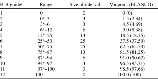
TABLE 1. Horsfall-Barratt (H-B) scale (15) showing the grades, ranges for the grades, H-B midpoints, and ELANCO midpoints (34)
H-B gradea Range Size of interval Midpoint (ELANCO)
1 0 0 0 (0)
2 0+–3 3 1.5 (2.34)
3 3+–6 3 4.5 (4.69)
4 6+–12 6 9.0 (9.38)
5 12+–25 13 18.5 (18.75)
6 25+–50 25 37.5 (37.50)
7 50+–75 25 62.5 (62.50)
8 75+–87 13 81.5 (81.25)
9 87+–94 6 91.0 (90.62)
10 94+–97 3 96.5 (95.31)
11 97+–100 3 98.5 (97.66)
12 100 0 100.0 (100)
a Horsfall and Barratt numbered the scale in two different ways, depending on
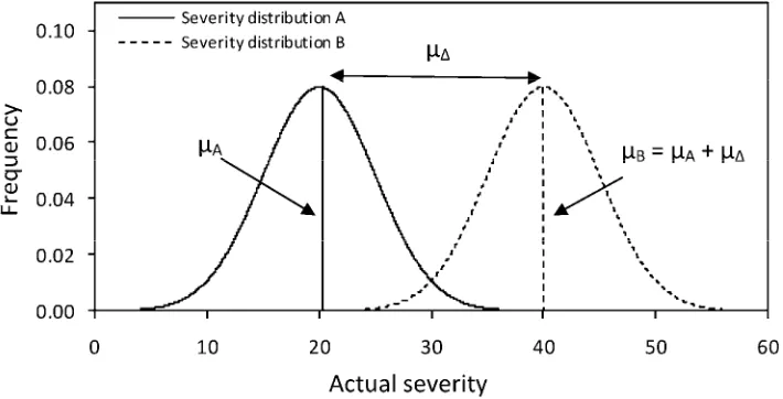
and treatment B, then, at time t, the epidemics have developed a particular leaf severity population distribution for each treatment (Fig. 1) which we assumed to be normal distributions. The disease severity distribution of treatment A has mean µA and treatment B
has mean µB = µA + µΔ, where µΔ represents the difference
be-tween the means of the two severity distributions and, thus, re-flects the treatment difference. Then, µΔ = 0 implies that the
treatments did not result in any effect and, therefore, the mean disease severities are the same; µΔ > 0 or < 0 implies that the
treatment affected the epidemic such that a difference in mean severity developed. Without loss of generality, we only considered µΔ > 0. The two hypothetical populations of diseased leaves, A
and B, are assumed to have an equal standard deviation (ϕ).
Sampling. To simulate disease severity estimation to the nearest percent by raters, n samples were taken randomly from each of the two disease severity distributions, A and B. These are the actual severities of the 2n samples. Next, we determined the rater observed severity for each of these actual severities. This was achieved for each of the 2n samples separately by drawing from the log-normal distribution with the actual severity as the mean of the distribution, µactual. This gives the rater-observed
severities for the n samples from each of the distributions. To simulate observations using the H-B scale, the data derived above were converted to the appropriate grade on the H-B scale (1 to 12) and grade numbers used for the nonparametric analysis (Mann-Whitney U test). These grade data were subsequently converted to the appropriate midpoint value for that grade for analysis with the parametric test (t test). Thus, three sets of data were generated from the simulated assessment process that mimics NPE and H-B scale assessments, as follows: (i) n
observations from the disease severity distribution with treatment A and n observations from treatment B, mimicking NPEs of disease severity by direct observation of the symptoms by a rater; (ii) n observations from the disease severity distribution with treatment A and n observations from treatment B, mimicking the use of the H-B scale; and (iii) n observations from the disease severity distribution with treatment A and n observations from treatment B using the H-B scale and subsequently converting the grade number to the midpoint severity of that interval range.
Testing. Each of the three sets of data was tested with the aim of detecting differences in the mean severity of the severity distributions resulting from the two treatments (A and B). For data set (i) and (iii), we used the two-sample t test, with the H0
being that the means of the two samples are equal. For data set (ii), we used the Mann-Whitney U test. The H0 of this test was
that the samples were drawn from the same distribution. The threshold for the rejection of H0 was set at P = 0.05. The choice of
a P value of 0.05 was arbitrary; there are advantages and disadvantages to increasing strength (i.e., 0.1, 0.05, or 0.01) but, here, we were concerned only with the relative difference be-tween the two methods (NPE and H-B) and not with the strength of the test (i.e., we were not trying to disprove an H0).
Further-more, by convention, P = 0.05 is the most widely used P value. Thus, the output variable was the probability to reject the H0, and
the aim was to investigate whether this probability was influenced by the way the observations were obtained (i.e., by NPEs or by using the H-B scale). To calculate the probability that the H0 is
rejected, the procedure outlined above was repeated 10,000 times unless stated otherwise and the t or Mann-Whitney U test performed each time. The proportion of occasions that the H0 was
rejected in these 10,000 tests was plotted against various param-eters (P value, magnitude of severity population mean, difference between severity population means, magnitude of severity population standard deviation, sample size, and rater ability).
RESULTS
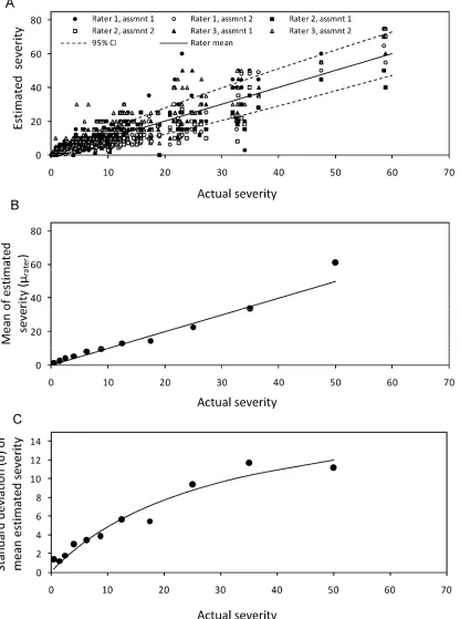
Characteristics of the real and simulated data. The mean severity calculated from the three rater estimates showed a linear relationship with the actual disease severity (Fig. 2B). Because the estimated parameter, θ in equation 1, was not significantly different from unity (P < 0.001), we have used θ = 1. This value implies that the average rater-observed severity equals the actual severity (Fig. 2B), although a tendency to overestimate disease at actual severities <10% is common (4,35). The linear relationship is in agreement with other studies (3,25,29). That θ = 1 shows that the rater has no systematic bias toward over- or underestimation (i.e., the rater mean is an accurate estimate of the actual mean).
The hyperbolic function described the relationship between the standard deviation of the rater mean NPEs and the actual mean disease severity accurately (Fig. 2C). Thus, the standard deviation of the rater mean NPEs increased almost linearly with actual severity at low actual severity but, for larger actual severity, the slope of the relationship decreased with increasing actual severity. Other studies have found that the standard deviation of the mean severity initially increases but that rate of increase declines between 12 and 25% mean disease severity (9,11).
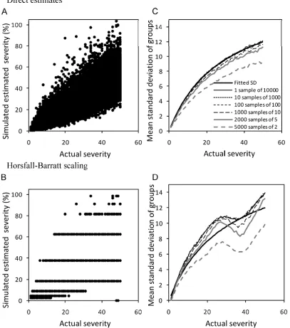
Based on the lognormal distribution of generalized rater ability and the parameters described in the previous section, 10,000 NPEs were taken from 0 to 50% severity in 1% increments (Fig.
Fig. 1. Example of the hypothetical population distributions used to test nearest percent estimates (NPE) and the Horsfall-Barratt (H-B) scale for detecting differences. We were interested in knowing whether a random sample taken from each can detect the difference in the two distributions when NPEs are used, and when these are converted to H-B midpoint values. The parameters are the ones referred to in Figures 4 to 8. The null hypothesis (H0) is that the two distributions
3A). The standard deviation of the mean of various sample sizes is generally in close agreement with the actual rater standard deviations (Fig. 3B). Only if sample size was particularly small (for example, two observations) was the standard deviation low throughout the range of actual disease simulated in this study (0 to 50% area infected). The underestimation of the standard deviation with small sample size is due to diminished outlier effects.
If these estimates are converted to the H-B midpoint values (Fig. 3C), the standard deviation clearly has characteristics differ-ent from those calculated from the NPEs (Fig. 3D). The standard deviation tends to be larger or smaller when using the H-B scale for all sample sizes. Only at low actual disease severity (<20%) where interval ranges are small is the standard deviation close to the rater standard deviation. Sample sizes ≥5 tended to have larger standard deviations compared with the rater standard deviation,
Fig. 2. A, Estimated disease severity data by three raters on two occasions assessing each of 200 grapefruit leaves infected with citrus canker (95% confidence limits are shown). B, Relationship between the mean estimated severity and the actual severity (µrater = θactual, r2 = 0.96). C, Relationship between the standard
deviations of the estimated means and the actual severity (hyperbolic fit, σ = αµactual/β + µactual, parameters α = 19.08, standard deviation (s.d.) = 3.19; β= 29.65,
except in the region of the midpoint of the largest interval size (midpoint value 37.5%), where a dip occurred and most groups had a smaller standard deviation. Similar to the standard deviation from the NPEs, only sample sizes of n = 2 had consistently smaller standard deviation throughout the range 0 to 50% area infected.
From these results, showing the effect of NPEs and the H-B scaled data on the estimated standard deviation of the mean estimate, the ability of these two different data to differentiate means is most likely different at severities of 20 to 50+%. The
information that has been published on the frequency of different severities on individual leaves suggests that these disease severities are common in many pathosystems in the field (11,21). Therefore, this range of severities was used to illustrate the differences in hypothesis testing between the two assessment methods.
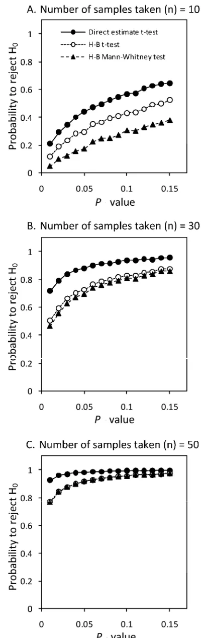
Hypothesis testing. Probability level. As expected, a larger P
value increased the probability to reject H0 when this hypothesis
was false (Fig. 4). Although the trends were similar for both NPEs and H-B scaled data, NPEs of disease severity invariably had a greater probability to correctly reject the H0 compared with H-B
scaled data. At a given P value, larger sample sizes increased the probability to reject H0 when H0 was false with both NPEs and
H-B scaled data; however, with small sample sizes, NPEs have a greater probability to reject H0 (when H0 is false). Particularly at
small sample sizes, the nonparametric Mann-Whitney U test re-sulted in the lowest probability compared with the t test. At sample sizes of ≥50, the two tests had equal probabilities and the superiority of NPEs was marginal.
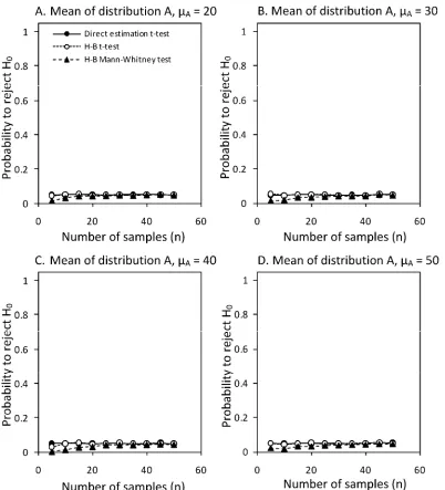
When populations are identical (i.e., no treatment difference).
When the severity distributions of the two treatments are the same, meaning µΔ = 0 (Fig. 5A to D), the t test rejects the H0
(being that µΔ = 0) although it is true (a type I error) in ≈5% of the
cases. This closely agrees with the choice of a P value of 0.05. There is no effect of sample size on this probability. There seems to be no difference between the data generated using the H-B scale and the data generated by NPE observations. As noted, at lower severity (<20%), the standard deviations of the estimates of the two methods are in close agreement (Fig. 3) and, thus, the probability of rejecting H0 when the populations are the same and
the mean severity low are similar, and close to 0.05, for both disease-assessment methods (data not shown). Applying the nonparametric Mann-Whitney U test to the H-B scale data resulted in a slightly smaller probability to reject the H0 when it is
true for H-B scaled data at lower replication.
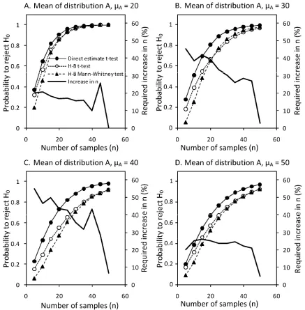
Different population means and the effect of sample size. As is
to be expected, increased sample size increased the probability to reject H0 (being that µΔ = 0) when this hypothesis is false (Fig. 6)
(i.e., there is a difference in mean disease severity between the two treatments). This holds for both assessment methods and both tests applied; however, NPEs of disease severity have a greater probability to correctly reject the H0 compared with H-B scale
data. Applying the nonparametric Mann-Whitney U test always resulted in the lowest probability to correctly reject the H0 when
this hypothesis is false.
The bold black lines in Figure 6A to D show the percent increase in the sample size using the H-B scale compared with NPEs needed to attain the same probability to reject the H0. In the
most extreme cases, it is necessary to take 50% more samples when using the H-B scale to obtain the same probability to correctly reject the H0 compared with NPEs.
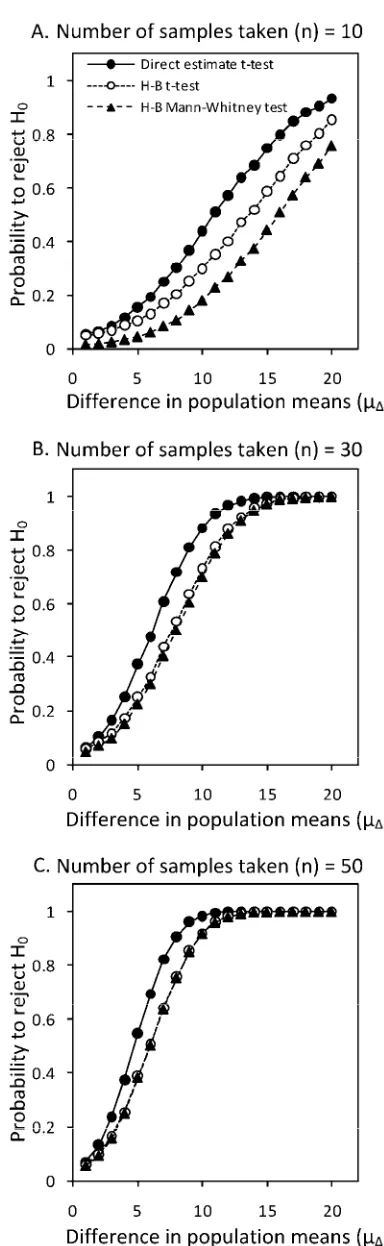
Magnitude of the population difference and the effect of sample
sizes. As expected, the greater the difference between the two
severity distribution means, µΔ, the greater the probability to reject
H0, a trend which holds for both assessment methods at all sample
sizes tested (Fig. 7). As previously noted, larger sample sizes resulted in greater probability to reject H0 (when H0 was false).
NPEs had a higher probability to reject H0 when H0 was false at
small sample sizes although, with greater sample size, this effect was minimal. The trends were similar for both the parametric t
test and nonparametric Mann-Whitney U test.
The effect of the standard deviation of the severity distribution
with different sample sizes. As might be expected, when the
standard deviation (ϕ) of the severity distribution is large (vari-able populations), there is a small probability to reject the H0
when H0 is false using either NPEs or when the H-B scale is small
(Fig. 8). Larger sample sizes increase the probability to reject H0
when H0 is false; however, with smaller sample sizes, NPEs have
a greater probability to reject H0, (when H0 is false), particularly
when standard deviations are small, and was similar for both the parametric and nonparametric tests.
The underlying population distribution affects the mean, median, and standard deviation of the mean, although the effect of using the H-B scale should be the same regardless of the distribution type. However, as population (and sample) variability increases (in wide or nonnormal distributions), the contribution of the H-B scale to sample variability will be relatively small compared with the amount of variability inherent in the sample— hence, as the standard deviation increases, probability to reject H0
(when H0 is false) declines and becomes similar for both methods
of assessment (Fig. 8).
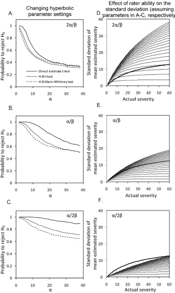
Rater ability. The parameters in equation 2 relate to rater
abil-ity. The parameter α is the maximum standard deviation of the rater-observed disease severity. The ratio α/β is the slope of the relation between actual severity and the standard deviation of the rater’s observation for low disease severities. Thus, an inaccurate rater will have a large value for α as well as large value for α/β. An accurate rater will have a small value for α and α/β. “Accurate” is used here to describe the closeness of individual estimates to the actual disease severity on that leaf (31) and not
Fig. 4. Effect of changing the P value (0.01 to 0.15) on the probability of rejecting the null hypothesis at various sample sizes (A,n = 10; B,n = 30; C, n = 50) at mean disease severity of population A (µA = 40). Hypothesis test
the accuracy of the mean value, which can be affected by rater bias. The accuracy of the individual estimates affects the variance of the mean. This study does not address error due to rater bias or bias in the mean value caused by the scale.
Our results, based on 10,000 simulations each, show that, for a very inaccurate rater (Fig. 9A for larger values of α), there is little difference in the probability to reject H0 for NPEs or for H-B
scaled data. The probability to reject H0 is small for an inaccurate
rater, and our results show that such raters might equally well use the H-B scale or take NPEs. As a result, the standard deviations associated with NPEs by inaccurate raters (from α = 2 to 38 for 2α/β) mostly exceed the standard deviations of the original mean rater estimates (Fig. 9D, shown by the bold black lines).
At the other extreme (Fig. 9C), data gathered by very accurate raters almost always lead to the rejection of H0 (when H0 is false)
when NPEs are used but using the H-B scale is detrimental to the probability to reject H0. This is reflected in the standard
deviations of the NPEs (Fig. 9F), which are smaller (α/2β) than the original mean rater estimates standard deviation (α/β).
Finally, average raters (Fig. 9B) with declining accuracy show similar trends but the ability to reject H0 when H0 is false is still
higher for average raters using NPEs compared with the H-B scale, and the standard deviations of the estimates are closer to the standard deviations of the original mean rater estimates (Fig. 9E).
DISCUSSION
The generalized rater distribution. We developed a mathe-matical description of the distribution of rater-estimated disease severities using the lognormal distribution. Bock et al. (4) used the normal distribution to describe the frequency of estimates compared with actual values but the lognormal distribution has the advantage that the tails do not tend to infinity, which is more realistic for estimation of a disease on the percent scale (0 to 100%). The use of the log-normal distribution to characterize rater variability in severity estimation up to 50% severity is new. Other distributions, such as the logit-normal, might also yield appropriate descriptions of disease severity, especially at 50 to
Fig. 5. Effect of sample size (n = 5–50) on the probability of rejecting the null hypothesis (H0) at various mean disease (µA, µB) severities (A, 20; B, 30; C,40; and
D, 50% disease severity) assuming no difference between the population means (µΔ = 0). Hypothesis test was performed on simulated nearest percent estimates and Horsfall-Barratt (H-B) scaled data. Both data sets were analyzed using a t test and, in addition, the H-B scaled data were analyzed using the Mann-Whitney U
100% severity; although we don’t believe it will make a differ-ence to the conclusions, it is something to consider in future work.
The nonconstant relation between the actual disease severity and the standard deviation of the rater-estimated mean disease severity is implicit in several other studies (4,9–11,20). We described the relationship up to 50% actual disease as hyperbolic. Previous work suggests that standard deviation of the mean estimate is nonconstant with actual disease both with estimates of disease by the same individual (11) and by different individuals combined (5,9–11,20). For leaves with severity of 50 to 100%, the relationship was not characterized but the standard deviation will probably decline toward 100% severity. Other valid relationships will need to be developed when these characteristics have been established and, clearly, this is an area for future studies.
In our data set based on the mean value of several ratings (Fig. 2B), we found that the estimated mean severity equals the actual severity (determined using image analysis, θ = 1), confirming observations of a linear relationship found in other studies
(3,5,11,25,26,28,29). Therefore, we have used a generalized rater distribution describing a nonbiased rater. Our method does allow for biased raters to be described, simply by taking θ ≠ 1. However, we considered rater bias (23) and its effect on hypothesis testing to be beyond the scope of this article.
Interacting effects of population means, standard deviations and differences, the sample size, and rater ability on hy-pothesis testing. When population mean differences were gross, disease severity distributions particularly variable, and sample sizes ample, there was little difference between NPEs or the H-B scale data from a generalized rater for hypothesis testing. Our results also show that, for populations where the mean disease severity was <20%, there was little or no difference between H-B scale estimates or NPEs.
However, there are situations where using H-B scale-based data compared with using NPEs for hypothesis testing might result in a greater risk of failing to reject H0 when H0 is false, causing a
type II error. This implies that, in these situations, NPEs would be preferred to using the H-B scale; however, our results also show
Fig. 6. Effect of sample size (n = 5 to 50) on the probability of rejecting the null hypothesis (H0) at various mean disease (µA, µB) severities (A, 20; B, 30; C,40;
and D, 50% disease severity) assuming a difference between the population means (µΔ = 10). Hypothesis test was performed on simulated nearest percent estimates and Horsfall-Barratt (H-B) scaled data. Both data sets were analyzed using a t test and, in addition, the H-B scaled data were analyzed using the Mann-Whitney U test. Population fixed values were ϕ = 5, with a probability threshold of rejecting H0of 0.05. The bold black line shows the required increase in sample
Fig. 7. Effect of increasing difference between the population means (µΔ = 2 to 20) on the probability of rejecting the null hypothesis (H0) at various sample
sizes (A,n = 10; B,n = 30; and C,n = 50) at mean disease severity of popu-lation A (µA = 40). Hypothesis test was performed on simulated nearest
percent estimates and Horsfall-Barratt (H-B) scaled data. Both data sets were analyzed using a t test and, in addition, the H-B scaled data were analyzed using the Mann-Whitney U test. Assumed fixed values were ϕ= 5, with a probability threshold of rejecting H0 of 0.05.
Fig. 8.Effect of increasing disease severity population distribution standard deviation (ϕ = 2 to 20) on the probability of rejecting the null hypothesis (H0)
at various sample sizes (A,n = 10; B,n = 30; and C,n = 50) at mean disease severity of population A (µA = 40). Hypothesis test was performed on
that, if the H-B scale is used and it is possible to take up to a 50% larger sample compared with the NPE sample size, then both methods have a similar probability to reject H0 when H0 is false.
These results confirm speculative discussion by Nutter and Esker (26) on the likelihood that added sample units are required to
achieve a predetermined level of precision of the mean when using the H-B scale.
Interacting with the mitigating effect of sample size, the factors that influence the probability of a type II error include the variability of the population (described by the standard deviation),
Fig. 9. Effect of rater ability on the probability of rejecting the null hypothesis (H0) at three different parameter settings (A, 2α/β; B,α/β; and C,α/2β) for
estimating rater standard deviation (s.d.). Hypothesis test was performed on simulated nearest percent estimates and Horsfall-Barratt (H-B) scaled data. Both data sets were analyzed using a t test and, in addition, the H-B scaled data were analyzed using the Mann-Whitney test. Assumed sample size (n) = 25, mean of population A (µA) = 40, difference between populations (µΔ) = 10, and s.d. (ϕ) = 5, with a threshold for rejecting H0of 0.05. The resulting calculated s.d. data
population means, population mean differences, and rater ability. However, it is pertinent to note that, if population variability is large, the effect of the H-B scale will be relatively small compared with sample variability, resulting in risk of a type II error being similar for analyses based on NPEs or H-B scale data (Fig. 8).
In this study, we assumed that the NPE was invariably in the correct H-B interval. Although raters might not always rate severity in the correct interval (10,11,22), this tendency has not been characterized; therefore, we describe a “best-case” scenario. Thus, estimates of disease severity by an inaccurate rater were not improved by taking NPEs compared with the H-B scale because the variance of the sample means were large using either method. However, raters of average ability using NPEs provided data with a higher probability of rejecting H0 when H0 was false. Thus, on
average, the NPEs of disease, particularly in the mid-range of the H-B interval scale, are better than what can be achieved by applying a grade or midpoint value. Raters who happen to be experienced, particularly accurate, highly trained, or who use standard area diagrams to improve the accuracy of each estimate (1,5,17,28,29) will provide NPEs that are most often much better than can be achieved with H-B scaled data. This might even be so at lower disease severities (<20%) because they will, on average, provide estimates closer to the actual values compared with H-B grades or midpoints in these ranges. Inevitably, in rating disease, inappropriate grades are chosen (22). Furthermore, if there is consistent bias, the mean value will be less accurate. A remaining need is to characterize how raters apply the grade directly, and identify the effect of these characteristics on hypothesis testing.
In all cases, increasing sample size improves the probability of rejecting H0 when H0 is false but, as noted above, if the H-B scale
is used and assuming no bias, up to 50% more samples are required to achieve a comparable probability. In defense of Horsfall and Barratt (15), they did state the need for substantial sample size when using the scale (15,16), and they never advocated basing the sample on a single or few estimates within a plot, and recommended a minimum of at least 20 individual assess-ments to achieve an accurate estimate of the mean. Additional sampling units cost resources (26,27), and it might be argued that taking grade data is much faster than taking NPEs, although this has not been demonstrated.
Hypothesis testing and the H-B scale. Many aspects of plant pathology, including comparing the effects of fungicide treat-ments and studying yield loss; cultural, agronomic, and manage-ment factors; disease resistance; and developmanage-ment of epidemics, rely on hypothesis testing. There are situations where the characteristics of the populations being tested and the rater ability (especially if sample sizes are inadequate) can increase the risk of a type II error when the H-B scale is used relative to NPEs. However, it should be noted that NPEs are error prone, too, and can result in faulty hypothesis testing (32), although to a lesser degree in the situations mentioned above.
Although the H-B scale can cause elevated type II error, it does not appear to influence the rate of type I error situations in hypothesis testing based on disease severity assessments. When the severity distributions of the two treatments were the same (µΔ = 0), the t test rejected the H0 at the same rate for both the
H-B scale and NPEs. Thus, both assessment methods committed a type I error in ≈5% of the cases by rejecting H0 when H0 was true,
closely agreeing with the choice of a P value of 0.05. In addition, these data were run at a P value of 0.1 and the type I error rate was 10%, as expected (data not shown), and the relationships among all these data tested at 0.05% remained similar when the P
value of 0.1 was used. Thus, there was no discernible qualitative effect of the H-B scale at different P values on the ability to reject H0 when H0 was false (Fig. 4).
Some general comment on hypothesis testing in relation to the H-B scale and other nonlinear scales for estimating dis-ease. Hypothesis testing was based on the t test. The t test is a
parametric test that makes some basic assumptions about the data, including normality, independence between samples, absence of outliers, and equal variances in relation to sample size. For this reason, a normal distribution of disease severity was assumed. There is limited information available on the frequency distri-bution of severity (percent area infected) on leaves of diseased plants (23), although it is known to change with mean disease severity and the point in the epidemic (11,21). The frequency distribution of diseased leaf severity can affect the accuracy of mean estimates using interval scales with different numbers of classes (11,20) but it is unlikely that differences in the population distributions would change the underlying effects of the H-B scale on sample variance that we describe here. Regardless of the underlying severity distributions, in experiments where analysis is based on several replicates, each being based on a large sample size, the central limit theorem states that the distribution of the means approximates to normal and, thus, the assumptions of parametric analysis are acceptable.
Other parametric tests make similar assumptions of normality and should be used only where interval scales have equal intervals on a continuous scale (37). Previous work has demonstrated the bias resulting from directly averaging the logarithmically based H-B scale data without first converting back to a percent (34). However, a nonparametric test is more appropriate for unequal interval-sized grade data; therefore, we analyzed the H-B scale grade data using the Mann-Whitney U test alongside the t test used for the midpoint values and found that the nonparametric test had a larger probability of a type II error compared with using the H-B scale midpoint percentages or the NPE data. This is to be expected because nonparametric tests are generally less powerful than parametric tests based on ratio level data.
Interval scales might be used to obtain data on disease severity for several purposes (surveys, hypothesis testing, forecasting, and so on). Some suggested modifications to the H-B scale to use for estimates of disease at a plot level based on a single sample might be too complex (1) to usefully apply in the field, because there are too many grades and the potential advantage of speed would be lost. Other nonlinear scales used include seven- or eight-category intervals with unequal interval sizes (11,20). Other suggestions for additional grades in the H-B scale have been made (7,18,25, 26), and many others scales developed to rate disease (36). Par-ticularly where disease severity data are to be used for hypothesis testing, our results suggest that it is desirable that a scale reflect the approximate ability of a rater. A disease scale with 5% increments might do this (25,26) although, at low disease severity, additional grades would be useful (for example, 0, 0.1, 1.0, 2.5, 5.0, 7.5, 10.0, 15.0%…) because the human eye appears more capable of differentiating disease at low severity (3,5,11,19). Furthermore, it can be argued that, for much epidemiological work, it is disease at low severity that needs to be most accurately estimated because these assessments form the basis for obtaining parameters that might be used in projecting epidemic develop-ment. Simulation modeling can usefully be applied to test and compare the use of different scales for disease assessment under different scenarios.
It has not been established how much time can be saved using a disease severity scale compared with NPEs. Direct application of the H-B scale is practiced (10,31) and incorrect grading of disease severity can lead to additional error (22). There is also some evidence that direct use of the H-B scale might result in a “linearizing” of the log-scale intervals (10), which would lead to further bias in the mean value. These tendencies would increase error of the mean estimates but they have not been sufficiently characterized. In this study, as in some others (2,25), we con-verted the NPE to the H-B scale, thereby guaranteeing that the NPE was graded correctly.
many situations where the two methods are equally good for hypothesis testing but the H-B scale was never better than NPEs for comparing treatments, and can result in less precise data leading to a greater risk of type II error (2,10,25,26). Increasing the sample size reduces this risk. However, an NPE has an advantage in that “…it allows observed differences to be recorded and used” (18). Observed differences are not subject to additional error by rescaling, and can be revisited as an honest repre-sentation of the rater’s assessment of severity which might be useful to posterity.
ACKNOWLEDGMENTS
We thank U. Albrecht and D. Flinn (United States Department of Agriculture–Agricultural Research Service–USHRL, Ft. Pierce, FL) for translating from German some of the original papers referenced in this article.
LITERATURE CITED
1. Berger, R. D. 1980. Measuring disease intensity. Pages 28-31 in: Proc. E. C. Stakman Commemorative Symp. Crop Loss Assessment. University of Minnesota Misc. Publ. 7, St Paul.
2. Bock, C. H., Gottwald, T. R., Parker, P. E., Cook, A. Z., Ferrandino, F., Parnell, S., and van den Bosch, F. 2009. Horsfall-Barratt scaling and replicated severity estimates of citrus canker. Eur. J. Plant Pathol. 125:23-38.
3. Bock, C. H., Parker, P. E., Cook, A. Z., and Gottwald, T. R. 2008. Visual assessment and the use of image analysis for assessing different symptoms of citrus canker on grapefruit leaves. Plant Dis. 92:530-541.
4. Bock, C. H., Parker, P. E., Cook, A. Z., and Gottwald, T. R. 2008.
Characteristics of the perception of different severity measures of citrus canker and the relations between the various symptom types. Plant Dis. 92:927-939.
5. Bock, C. H., Parker, P. E., Cook, A. Z., Riley, T., and Gottwald, T. R. 2009. Comparison of assessment of citrus canker foliar symptoms by experienced and inexperienced visual raters. Plant Dis. 93:412-424. 6. Chang, S. W., Chang, T. H., Abler, R. A. B., and Jung, G. 2007. Variation
in bentgrass susceptibility to Typhula incarnata and in isolate
aggressiveness under controlled environment conditions. Plant Dis. 91:446-452.
7. Chester, K. S. 1950. Plant disease losses: their appraisal and
interpretation. Plant Dis. Rep. (Suppl.) 190-198 (S193):190-362.
8. Dorman, E. A., Webster, B. J., and Hausbeck, M. K. 2009. Managing
foliar blights on carrot using copper, azoxystrobin, and chlorothalonil applied according to TOM-CAST. Plant Dis. 93:402-407.
9. Forbes, G. A., and Jeger, M. J. 1987. Factors affecting the estimation of disease intensity in simulated plant structures. Z. Pflanzenkrankh. Pflanzenschutz 94:113-120.
10. Forbes, G. A., and Korva, J. T. 1994. The effect of using a Horsfall-Barratt scale on precision and accuracy of visual estimation of potato late blight severity in the field. Plant Pathol. 43:675-682.
11. Hau, B., Kranz, J., and Konig, R. 1989. Fehler beim Schätzen von
Befallsstärken bei Pflanzenanzenkrankheiten. Z. Pflanzenkrankh. Pflanzenschutz 96:649-674.
12. Herbert, T. T. 1982. The rationale for the Horsfall-Barratt plant disease assessment scale. Phytopathology 72:1269.
13. Horsfall, J. G. 1945. Fungicides and Their Action. Annales Cryptogamica et Phytopathologici, Vol. II. Chronica Botanica, Waltham, MA.
14. Horsfall, J. G. 1986. This week’s citation classic: Horsfall J. G., and Barrat, R. W. An improved grading system for measuring plant disease. Phytopathology 35:655. 1945. Current Contents (Agriculture, Biology and Environmental Sciences), 15, 14.
15. Horsfall J. G., and Barratt, R. W. 1945. An improved grading system for measuring plant disease. (Abstr.) Phytopathology, 35:655.
16. Horsfall, J. G., and Cowling, E.B. 1978. Pathometry: the measurement of plant disease. Pages 120-136 in: Plant Disease: An Advanced Treatise, Vol. II. J. G. Horsfall and E. B. Cowling, eds. Academic Press, New York. 17. James, W. C. 1971. An illustrated series of assessment keys for plant
diseases, their preparation and usage. Can. Plant Dis. Surv. 51:39-65.
18. James, W. C. 1974. Assessment of plant disease losses. Annu. Rev.
Phytopathol. 12:27-48.
19. Koch, H., and Hau, B. 1980. Ein psychologischer aspect beim schatzen von pflanzenkrankheiten. Z. Pflanzenkrankh. Pflanzenschutz 87:587-593. 20. Kranz, J. 1970. Schatzklassen fur krankheitbefall. Phytopathol. Z.
69:131-139.
21. Kranz, J. 1977. A study on maximum severity in plant disease. Pages 169-173 in: Travaux dédiés à G. Viennot-Bourgin.
22. Kranz, J. 1988. Measuring plant disease. Pages 35-50 in: Experimental Techniques in Plant Disease Epidemiology. J. Kranz and J. Rotem, eds. Springer-Verlag, New York.
23. Madden, L. V., Hughes, G., and van den Bosch, F. 2007. The Study of Plant Disease Epidemics. American Phytopathological Society, St. Paul, MN.
24. Nita, M, Ellis, M. A., and Madden, L. V. 2003. Effects of temperature, wetness duration, and leaflet age on infection of strawberry foliage by
Phomopsis obscurans. Plant Dis. 87:579-584
25. Nita, M, Ellis, M. A., and Madden, L. V. 2003. Reliability and accuracy of visual estimation of Phomopsis leaf blight of strawberry. Phytopathology 93:995-1005.
26. Nutter, F. W., Jr., and Esker, P. D. 2006. The role of psychophysics in phytopathology. Eur. J. Plant Pathol. 114, 199-213.
27. Nutter, F. W., Jr., and Gaunt, R. E. 1996. Recent developments in methods for assessing disease losses in forage/pasture crops. Pages 93-118 in: Pasture and Forage Crop Pathology. S. Chakraborty, ed. ASA, CSSA, and SSSA, Madison, WI.
28. Nutter, F. W., Jr., Gleason, M. L., Jenco, J. H., and Christians, N. C. 1993. Assessing the accuracy, intra-rater repeatability, and inter-rater reliability of disease assessment system. Phytopathology 83:806-812.
29. Nutter, F. W., Jr., and Schultz, P. M. 1995. Improving the accuracy and precision of disease assessment: selection of methods and use of computer-aided training programs. Can. J. Plant Pathol. 17:174-178. 30. Nutter, F.W., Jr., Teng, P. S., and Shokes, F. M. 1991. Disease assessment
terms and concepts. Plant Dis. 75:1187-1188.
31. O’Brien, R. D., and van Bruggen, A. H. C. 1992. Accuracy, precision, and correlation to yield loss of disease severity scales for corky root of lettuce. Phytopathology 82:91-96.
32. Parker, S. R., Whelan, M. J., and Royle, D. J. 1995. Reliable measurement of disease severity. Asp. Appl. Biol. 43:205-214.
33. Pfleeger, T. G., and Mundt, C. C. 1998. Wheat leaf rust severity as affected by plant density and species proportion in simple communities of wheat and wild oats. Phytopathology 88:708-714.
34. Redman C. E., King, E. P., and Brown, I. F., Jr. 1969. Tables for
Converting Barratt and Horsfall Rating Scores to Estimated Mean Percentages. Elanco Products, Indianapolis, IN.
35. Sherwood, R. T., Berg, C. C., Hoover, M. R., and Zeiders, K. E. 1983. Illusions in visual assessment of Stagonospora leaf spot of orchardgrass. Phytopathology 73:173-177.
36. Slopek, S. W. 1989. An improved method of estimating percent leaf area diseases using a 1 to 5 disease assessment scale. Can. J. Plant Pathol. 11:381-387.
37. Snedecor, G. W., and Cochran, W. G. 1989. Statistical Methods, Eighth Edition. Iowa State University Press.
38. Watson, G., Morton, V., and Williams, R. 1990. Standardization of disease assessment and product performance reporting: an industry perspective. Phytopathology 74:401-402.