Resource Optimization in Multi Tier HetNets Exploiting Multi Slope Path Loss Model

Resource Optimization in Multi-Tier HetNets

Exploiting Multi-Slope Path Loss Model

Hamnah Munir, Syed Ali Hassan, Haris Pervaiz, Qiang Ni, and Leila Musavian

Abstract—Current resource allocation techniques in cellular networks are largely based on single-slope path loss model, which falls short in accurately capturing the effect of physical environment. The phenomenon of densification makes cell pat-terns more irregular therefore the multi-slope path loss model is more realistic to approximate the increased variations in the links and interferences. In this paper, we investigate the impacts of multi-slope path loss models, where different link distances are characterized by different path loss exponents. We propose a framework for joint user association, power and subcarrier allocation on the downlink of a heterogeneous network (HetNet). The proposed scheme is formulated as a weighted sum rate maximization problem, ensuring the users’ quality-of-service (QoS) requirements namely, users’ minimum rate, and the base stations’ (BSs) maximum transmission power. We then compare the performance of the proposed approach under different path loss models to demonstrate the effectiveness of dual-slope path loss model in comparison to single-slope path loss model. Simulation results show that the dual-slope model leads to significant improvement in network’s performance in comparison to the standard single-slope model by accurately approximating the path loss exponent dependence on the link distance. Moreover, it improves the user offloading from macrocell BS to small cells by connecting the users to nearby BSs with minimal attenuation. It has been shown that the path loss exponents significantly influence the user association lying across the critical radius in case of the dual-slope path loss model.

Index Terms—Heterogeneous network, weighted sum-rate, multi-slope path loss model, user association, load balancing, resource optimization.

I. INTRODUCTION

To manage the exponential growth of wireless data traffic [1] and to enable the high data rates, network densification has drawn tremendous attention in the future fifth generation (5G) networks [2]. Heterogeneous networks (HetNets) realize densification by deploying low-powered BSs to complement the conventional cellular network. HetNets have a great poten-tial to cope with the proliferation of wireless data traffic by allowing the fusion of technologies, frequency bands, diverse cell sizes and network architectures [3], [4]. HetNets ensure significant enhancement in the overall network performance complemented with high data rates and expanded cell cov-erage. Nevertheless, these advantages come along with new technical challenges which include hardware expenses, user H. Munir and S. A. Hassan are with the School of Electrical En-gineering & Computer Science (SEECS), National University of Sci-ences & Technology (NUST), Islamabad, Pakistan. e-mails: (14mseehmunir, ali.hassan)@seecs.edu.pk.

H. Pervaiz is currently with 5G Innovation Center (5GIC) at Univer-sity of Surrey, UK and during the work of this paper, he was with School of Computing & Communications, Lancaster University, UK. e-mail: [email protected]

Q. Ni is with School of Computing & Communications, Lancaster Univer-sity, UK. e-mail: [email protected]

L. Musavian is with School of Computer Science & Electronic Engineering, University of Essex, UK. e-mail: ([email protected])

association, interference management, radio resource manage-ment and energy efficiency (EE) [5], [6]. In order to optimize radio resources, some frameworks are proposed in [7], [8].

2169-3536 (c) 2016 IEEE. Translations and content mining are permitted for academic research only. Personal use is also permitted, but republication/redistribution requires IEEE permission. See Most of the existing works on the performance analysis

of cellular networks, especially the ones using optimization theory, use single-slope path loss model to characterize the propagation environment [20]. However, the massive data traffic and densification in the future wireless network lead to increasing network irregularities, which, in turn, elevate the variations in the links significantly [21]. In order to cater for these variations, many physical factors including link distances, ground reflections, scattering, and interferences, make path loss modeling a complex task in cellular networks. The standard path loss models are easy to study and analyze but they characterize all the links in a cell with a single path loss exponent (PLE), which lacks precision in a dense wireless network [22]. Performance degradation occurs as this model does not capture the dependence of the PLE on the link distance perfectly [23]. However, in the most recent works, this trend is shifted towards dual-slope path loss model, as presented in [24]–[26]. In [24], coverage probability and network throughput have been analyzed under multi-slope path loss model on the downlink of a cellular network. In [25], the authors investigate the path loss model incorporating both line-of-sight (LoS) and non line-of-sight (NLoS) transmission in small cell networks and compare it with standard path loss model. The paper further studies the impact of dual-slope path loss model on the coverage probability with varying small cell densities. This work was extended to user association in Het-Nets using dual-slope path loss model, in [26], which analyzed the effectiveness of biasing and uplink/downlink decoupling with dual-slope model on user association. This migration to dual-slope model is influenced by network densification and mmWave communications. The network densification causes more irregularities in cell patterns, which affects the inter-ference composition and thus, the links cannot be accurately approximated by a single PLE [27], [28]. The use of mmWave spectrum, ranging from 30-300 GHz, can improve the network performance but faces many challenges including sensitivity to blocking due to highly intermittent links [29]–[31]. Dual-slope path loss model has a great potential to better approximate the LoS and NLoS links, in mmWave systems, using different PLEs. Considering this simplest path loss model does not provide the precise dependence between the PLEs and the link distances, there is a need for more accurate path loss model to improve the performance in dense cellular networks, as discussed in [27].

Multi-slope models apply different PLEs for different link distances, which result in improved performance for dense networks, as shown in [24]. This model considers different slopes above and beyond the critical distance, which can be used to approximate the two regimes of LoS and NLoS links. The critical distance is the distance where the first Fresnel zone becomes obstructed and below this distance all links are LoS. This distance is also known as breakpoint distance where the slope changes and it can be calculated as given in [21], [32]. This distance is highly dependent on the antenna height and the Fresnel clearance zone starts expanding with the increase in the antenna height. This is because the increase in the antenna height pushes the obstructions in the Fresnel

zone farther. In addition to the antenna height, this distance is slightly dependent on the environment as well [33]. In case of mmWave communication, this distance is environment dependent random variable, which increases with low blocking environment, but can be approximated by taking the average LoS link distance [34]. The dual-slope model was first studied for LoS environment for free space reference distance model in [35] and for the indoor scenario in [36]. In [37], a dual-slope model has been proposed to reduce the root mean square (RMS) error between the local mean path loss samples and the path loss model, for NLoS environment.

According to the best of our knowledge, the resource allocation technique in a HetNet exploiting dual-slope path loss model has not been presented previously and there is no work in the literature that analyzes the network perfor-mance under difference slopes in different tiers of a HetNet, simultaneously. Most of the recent work on dual-slope path model have considered single-tier networks [22], [24], [25], [38]. Different from the existing works, this paper presents the analysis of the proposed resource optimization framework under different combinations of single-slope and dual-slope path loss models in a two-tier network.

Highlighting the importance of using an accurate approxi-mation of links in dense networks [24]–[27], this paper formu-late a joint user association, subcarrier and power allocation to maximize the weighted sum rate of a HetNet multi-tier downlink, while satisfying constraints on the BSs’ transmis-sion power and users’ quality-of-service (QoS) requirements. The proposed framework utilizes both single-slope and dual-slope path loss models. For better tractability, we transform the weighted sum rate maximization problem into a minimization problem using time sharing relaxation. We then prove that the transformed optimization problem is convex with respect to transmit power and subcarrier allocation variable using Hessian matrix. The optimal solution to the proposed optimiza-tion problem is derived by exploiting Karush–Kuhn–Tucker (KKT) conditions. The main contributions of this paper can be summarized as follows:

• We aim to maximize the weighted sum rate in the down-link of a multi-tier HetNet while considering user QoS re-quirement and maximum transmission power constraints. In contrast to the existing works such as [24]–[27], which highlight the importance of multi-slope model and ana-lyze coverage probability, our objective is to propose and analyze the QoS-aware resource optimization framework incorporating multi-slope path loss model in a multi-tier HetNet.

• The proposed framework is evaluated under different path loss models and we prove that dual-slope model improves the sum rate and EE of the network in comparison to the single-slope model. Since dual-slope model offloads the users to the closest BSs due to minimal attenuation, which increases the received signal strength, the better data rate can be achieved. As a result of better approximation of links in dual-slope model, the power consumption reduces and EE improves.

we show that when dual-slope path loss model is applied on small cells, the users connect to the nearby small cell BSs due to reduced attenuations and smaller PLE. Furthermore, we investigate the impact of PLEs on the performance of the network exploiting dual-slope path loss model and prove that the larger the NLoS PLE of a tier, the larger the attenuation and more users, residing outside the critical radius, offload to other tier. In essence, we show that the dual-slope model is beneficial for load-balancing in dense networks.

• The performance of a multi-tier HetNet using power minimization and weighted EE maximization techniques is also analyzed, under both single-slope and dual-slope path loss models. We prove that the dual-slope model performs better than the standard single-slope model in all approaches.

The rest of this paper is organized as follows. In Section II, we present the system model of the proposed framework and introduce the path loss models. In Section III, we formu-late joint subcarrier and power allocation on the downlink of a multi-tier HetNet as an objective function maximizing the weighted sum rate. Section IV shows the simulation results to demonstrate the performance of proposed scheme under single and dual-slope path loss models and Section V generalizes the conclusion drawn in the dual-slope case along with the concluding remarks.

II. SYSTEMMODEL

Consider the downlink of a two-tier HetNet composed of

M −1 picocell base stations (PBSs) overlaid on a macrocell. The macrocell base station (MBS) is represented by mo

whereas the set of all the base stations (BSs) in the system is given as M ={mo, m1, ..., mM−1}. Let N=

M−1

S

m=0 Nm be

the set of all users deployed uniformly over the entire area where Nm represents the set of users connected to the mth

BS. The bandwidth,B, is equally divided amongK identical subcarriers where K = {1,2,3, ..., K} be the set of all the subcarriers.

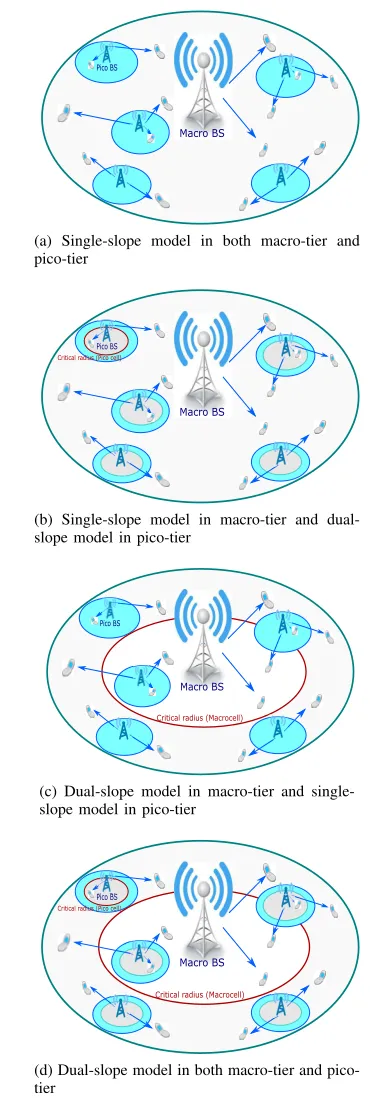
A snapshot of a two-tier HetNet consisting of picocells overlaid on a macrocell, with users uniformly scattered over the entire area, is shown in Fig. 1. Fig. 1(a) shows the scenario where all BSs use single-slope path loss model. On the other hand, Fig. 1(b) shows the scenario where MBS operates on single-slope path loss model, whereas all PBSs operate on a dual-slope path loss model. Fig. 1(c) shows the scenario where MBS operates on dual-slope path loss model, whereas all PBSs operate on single-slope path loss model. Fig. 1(d) shows the scenario where all BSs use dual-slope path loss model. These path loss models are explained in detail in Section II-A.

To maintain the QoS requirements of the users, a con-straint on the minimum achievable rate is applied. We assume that the minimum required rate is identical for all users and is equal to Rmin. Let ρn,m[k] {0,1} denote the subcarrier

allocation. If the subcarrier k of the mth BS is assigned to the nth user, ρn,m[k] = 1, otherwise ρn,m[k] = 0. The instantaneous achievable data rate (b/s/Hz) of the nth _user

Macro BS

Pico BS

(a) Single-slope model in both macro-tier and pico-tier

Macro BS Critical radius (Pico cell)

Pico BS

(b) Single-slope model in macro-tier and dual-slope model in pico-tier

Macro BS

Critical radius (Macrocell)

Pico BS

(c) Dual-slope model in macro-tier and single-slope model in pico-tier

Macro BS

Critical radius (Macrocell)

Critical radius (Pico cell)

Pico BS

(d) Dual-slope model in both macro-tier and pico-tier

Figure 1: A two-tier heterogeneous cellular network.

associated with BSmon each subcarrierk is given as

rn,m[k] =ρn,m[k]log₂(1 +γn,m[k]pn,m[k]), (1)

where pn,m[k] represents the power allocated to the kth

subcarrier for the user n at the BS m. Here, γn,m[k] is the

channel-to-noise ratio (CNR) of the nth _{user associated with}

themth_{BS on the subcarrierk and is defined as}

γn,m[k] = |hn,m[k]|

2

N0L(dn,m)

2169-3536 (c) 2016 IEEE. Translations and content mining are permitted for academic research only. Personal use is also permitted, but republication/redistribution requires IEEE permission. See where hn,m[k] represents the channel gain of the nth user

from themth_{BS on the subcarrier kandL(d}

n,m)is the path

loss between user nand BS m.

If usernis associated with BS m, then the total achiev-able rate of the user n over all the allocated subcarriers is given as

Rn =

X

m∈M

X

k∈K

rn,m[k]. (3)

A. Propagation Models

In this section, we present different path loss models to characterize the large scale fading in a network.

Definition 1 - Single-slope Path Loss Model: The

single-slope path loss model, L1(d), is given as

L1(d)[dB] = 20 log

_4π

λc

+ 10αlog(d) +ξ, (4)

wheredis the distance in meters,λccorresponds to the carrier

wavelength andαis the PLE. In (4), ξis a Gaussian random variable (RV) with zero mean and σ2 variance representing shadow fading. The single-slope path loss model generally falls short in accurately capturing the PLE dependence on the physical environment in dense and millimeter wave capable networks. These limitations lead to the consideration of dual-slope path loss model, which is described below.

Definition 2 - Dual-slope Path Loss Model: The

dual-slope path loss model is given by [26], [35]

L2(d)[dB] =

        

β+ 10α0log10(d) +ξ d≤rc

β+ 10α0log10(rc)

+10α1log

d rc

+ξ d > rc

, (5)

wherercis the critical radius of a cell, in meters.βrepresents

the floating intercept,α0 andα1 are the PLEs for below and beyondrc.

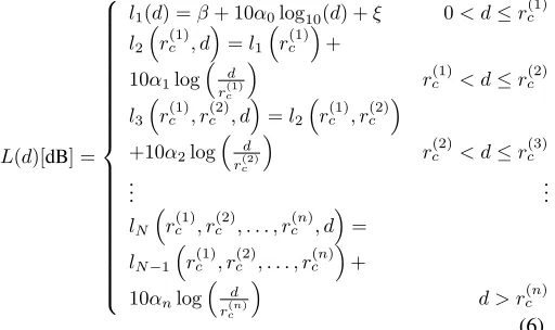
Definition 3 - N-slope Path Loss Model:The N-slope

path loss model is given as [24]

L(d)[dB] =                                           

l1(d) =β+ 10α0log10(d) +ξ 0< d≤r (1)

c

l2

r(1)c , d

=l1

r(1)c

+

10α1log

d rc(1)

r(1)c < d≤r(2)c

l3

r(1)c , r(2)c , d

=l2

r(1)c , rc(2)

+10α2log

d rc(2)

r(2)c < d≤r(3)c

..

. ...

lN

rc(1), r(2)c , . . . , r(cn), d

=

lN−1

r(1)c , rc(2), . . . , r(cn)

+

10αnlog

d r(cn)

d > r(cn)

,

(6) whereαn,n={0,1, .., N−1}, is the PLE such that0≤α0≤

α1 ≤... ≤αN−1. The critical distance is denoted as rc(n),

n={0,1, .., N−1}, such thatrc(0) ≤rc(1)≤...≤rc(N−1).

This model can be reduced to dual-slope path loss model with

N = 2.

Table I: The notations for different parameters used in this study.

Parameter Symbols

Set of Tiers I

Set of BSs M

Set of Users N

Set of Users associated with mth _{BS N} m

Index Set of Sub-carriers K Distance between nth_{user andm}th _{BS d}

n,m

Transmit Power pn,m[k]

Channel Gain hn,m[k]

Channel-to-noise Ratio γn,m[k]

Subcarrier Allocation Indicator ρn,m[k]

nth _{User Weight ω}

n

ith tier Biasing Factor θi

Critical Radius rc

Path Loss Exponent (Single-Slope) α

Path Loss Exponents (Dual-Slope) [α0, α1] Path Loss Exponents (N-Slope) [α0, ..., αN−1]

Floating intercept β

Minimum Rate Threshold Rmin mth _{BS Power Budget P}max m

III. PROPOSEDWEIGHTEDSUMRATEMAXIMIZATION SCHEME: ANOPTIMIZATIONAPPROACH

In this section, we propose a joint user association, subcarrier and power allocation scheme to maximize the weighted sum rate on the downlink of a two-tier HetNet. In this approach, we formulate weighted sum rate maximization as a single objective optimization problem (SOP) subject to the BSs’ maximum transmission power consumption and users’ minimum achievable rate. The performance of the proposed approach is then evaluated under different path loss models. The SOP is given as follows

max

ρ,p X

m∈M

X

n∈N

ωn

X

k∈K

ρn,m[k]log2(1 +γn,m[k]pn,m[k]),

s.t. C1:X

n∈N

X

k∈K

ρn,m[k]pn,m[k]≤Pmmax, ∀m.

C2:Rn≥Rmin, ∀n.

C3:X

n∈N

ρn,m[k]≤1, ∀k, m.

C4:ρn,m[k]∈ {0,1}, ∀n, k, m.

(7) where ωn represents the weight of the nth user such that 0 ≤ ωn ≤ 1. Here, C1 limits the maximum transmission

power of each BS toPmax

m . The Constraint C2 ensures that each

user gets at least the minimum required rate, i.e, Rmin. The

The maximization problem in (7) is a mixed integer programming (MIP) problem due to binary and continuous variables and is generally NP-hard. This optimization problem is also not convex with respect to (ρn,m[k], pn,m[k]). In order to achieve the convexity, we reformulate the optimization prob-lem, as in [39], by replacing xlog₂(1 +y)with xlog₂(1 +y_x), which is now convex in (x,y). The optimization problem in (7) becomes convex minimization problem and given as

min

ρ,p −

X

m∈M

X

n∈N

ωn

X

k∈K

ρn,m[k]log2

1 +γn,m[k]pn,m[k] ρn,m[k]

,

s.t. C1:X

n∈N

X

k∈K

ρn,m[k]pn,m[k]≤Pmmax, ∀m.

C2:Rn≥Rmin, ∀n.

C3:X

n∈N

ρn,m[k]≤1, ∀k, m.

C4:ρn,m[k]∈[0,1], ∀n, k, m.

(8) Here, the constraint C4 is relatively relaxed as the vari-ables are now continuous i.e., ρn,m[k]∈[0,1]by using time sharing and hence the optimization problem is convex. The convexity of the objective function with respect to optimiza-tion variables ρn,m[k] and pn,m[k] is proved. The proof of

convexity is given in detail in Appendix A. The Lagrangian of the objective function in (8) can be written as

L=−X

m∈M

X

n∈N

ωn

X

k∈K

ρn,m[k]log2

1 +γn,m[k]pn,m[k] ρn,m[k]

+X

m∈M

λm

X

n∈N

X

k∈K

ρn,m[k]pn,m[k]−Pmmax

!

+X

n∈N

ηn(Rmin−Rn) +

X

m∈M

X

k∈K

αm,k

X

n∈N

ρn,m[k]−1

!

+ X

m∈M

X

n∈N

X

k∈K

µn,m,k

(0−ρn,m[k]) +

X

m∈M

X

n∈N

X

k∈K

νn,m,k(ρn,m[k]−1),

(9) where ~λ = {λ0, λ1, ..., λM−1} and ~η = {η1, η2, ..., ηN} are

the Lagrange multiplier vectors associated with the maxi-mum transmit power and minimaxi-mum required rate constraints, respectively. The parameters α~ = {α1,1, α1,2, ..., αM−1,K}, ~

µ = {µ1,1,1, ..., µN,M−1,K} and~ν ={ν1,1,1, ..., νN,M−1,K}

are the Lagrange multiplier vectors associated with the exclu-sive subcarrier allocation at each BS. The above equation can be written, after few mathematical manipulation, as

L=−X

m∈M

X

k∈K

ρn,m[k]

X

n∈N

ωnlog2

1 +γn,m[k]pn,m[k] ρn,m[k]

+

ηnlog2(1 +γn,m[k]pn,m[k])

+X

m∈M

X

n∈N

X

k∈K

λmpn,m[k]ρn,m[k]+

X

m∈M

λmPmmax+

X

n∈N

ηnRmin+ X

m∈M

X

k∈K

αm,k

X

n∈Nm

ρn,m[k]−1

!

+X

m∈M

X

n∈Nm

X

k∈K

µn,m,k(0−ρn,m[k]) +

X

m∈M

X

n∈N

X

k∈K

νn,m,k

(ρn,m[k]−1)

(10)

The optimal solution must satisfy the KKT conditions

[40]. By taking the derivative of (10) w.r.tρn,m[k], we have

∇ρn,m[k]L=−ωn

log2

1 +γn,m[k]pn,m[k]

ρn,m[k]

−

γn,m[k]pn,m[k]

ln2 (ρn,m[k] +γn,m[k]pn,m[k])

−ηnlog2(1 +γn,m[k]

pn,m[k]) +λmpn,m[k] + αm,k−µn,m,k+νn,m,k

= 0,

(11)

Now, by taking the derivative of (10) with respect to Lagrange multipliers associated with subcarrier assignment, we get

αm,k∇αm,kL=αm,k

X

n∈N

ρn,m[k]−1

!

= 0, (12)

µn,m,k∇µn,m,kL=µn,m,k(0−ρn,m[k]) = 0, (13)

νn,m,k∇νn,m,kL=νn,m,k(ρn,m[k]−1) = 0. (14)

Eq. (11) can be rewritten as

ζn,m[k] =ωn

log₂

1 + γn,m[k]pn,m[k]

ρn,m[k]

−

γn,m[k]pn,m[k]

ln2 (ρn,m[k] +γn,m[k]pn,m[k])

+ηnlog2(1 +γn,m[k]

pn,m[k])−λmpn,m[k] =αm,k−µn,m,k+νn,m,k.

(15)

Using (13) and (14), we can say that the kth subcarrier is assigned to thenthuser by themthBS whenρn,m[k] = 1, giving µn,m,k = 0 and νn,m,k ≥ 0. Whereas, ρn,m[k] < 1

shows that the subcarrier k is not assigned to the nth user, thereforeµn,m,k = 0andνn,m,k = 0. Thus,

ζn,m[k]−αm,k=

≥0 ρn,m[k] = 1, = 0 ρn,m[k]<1.

(16)

From (12) and (16), it can be concluded that αm,k is

a constant for kth _{subcarrier at the m}th _{BS and the k}th

subcarrier must be assigned to the nth user associated with themthBS, which maximizes

nm=arg max n

{ζn,m[k]−αm,k}, ∀n∈N. (17)

Forρn,m[k] = 1, (17) becomes similar as solving

nm=arg max n

ωn[log2(1 +γn,m[k]pn,m[k])]

, (18)

wherern,m[k] =log2(1 +γn,m[k]pn,m[k])when the value of ρn,m[k] = 1.

Thus, from (18), the subcarrier assignment can be deter-mined as

ρn,m[k] =

(

1, nm=arg max n

{ωn(rn,m[k])}

0, otherwise. (19)

2169-3536 (c) 2016 IEEE. Translations and content mining are permitted for academic research only. Personal use is also permitted, but republication/redistribution requires IEEE permission. See ∇pn,m[k]L=−

γn,m[k]

ln2

_ω

n

1 +γn,m[k]pn,m[k]

ρn,m[k]

+

ηn

(1 +γn,m[k]pn,m[k])

+λmρn,m[k] = 0,

(20)

Using (20), the optimal power for thenthuser on thekth

subcarrier associated with themthBS , for a given subcarrier allocation, is given as

pn,m[k] =



 

 

ωn+ηn

ln2 λm

− 1

γn,m[k]

!+

, if(ρn,m[k] = 1)

0, otherwise,

(21) where[x]+=max(0, x).

The expression for optimal power allocation on each subcarrier has a semi-closed form in terms of Lagrangian multipliers. From (21), we can say the given power allocation is a modified water filling solution, where γn,m[k] is the channel gain and water level are determined by Lagrangian multipliers. These multipliers must satisfy KKT conditions.

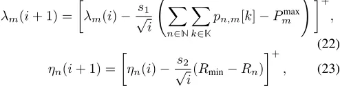
The Lagrangian multipliers can be updated according to

λm(i+ 1) =

λm(i)−√s1

i X

n∈N

X

k∈K

pn,m[k]−P_mmax

! +

,

(22)

ηn(i+ 1) =

ηn(i)−√s2

i(Rmin−Rn)

+

, (23)

where i is the iteration number and sj = 0√.1

i, j ∈ {1,2}.

This process of computing optimal power and subcarrier allocation along with Lagrangian multipliers are updated until convergence is achieved, guaranteeing optimal solution.

The complexity of the proposed approach to solve (8) is O(M × K × N) and with the accuracy re-quirement of δ = 10−3, the complexity becomes

O I×M×K×N×log₂(1_δ) where I is the number of iterations required until the algorithm converges. We observe that the proposed scheme has polynomial time complexity. The complexity of the proposed scheme is low in comparison to the complexity of the exhaustive search over all possible combinations.

A. Power Minimization Approach

For power minimization approach, the minimum achiev-able rate constraint for each user is met with equality, i.e.,

Rn = Rmin. The optimal water level (inverse) for achieving Rmin can be computed, using water filling equations, as

η_n=



2−

Rmin Y

k∈|Kn|

γn,m[k]





1

|Kn|

, (24)

where|Kn|={k∈K:γn,m[k]> ηn} is the subset of active

subcarriers for user n. More details about calculatingηn can

be found in Appendix B. The power allocation can be done using water level (inverse) η_n as

Table II: Simulation Parameters.

Parameter Value Parameter Value

α0(Pico-tier) 2 α1(Pico-tier) 3 α0(Macro-tier) 2.7 α1(Macro-tier) 3.9

α 3 β 38.45dB

σξ 6.9 dB fc 2GHz

pn,m[k] =

1

η_n −

1

γn,m[k]

+

. (25)

For a given subcarrier assignment, the optimal power can be calculated as

p∗_n,m[k] =min{p_n,m[k], pn,m[k]}, (26)

wherepn,m[k]is given by (21).

B. Weighted EE Maximization Approach

In this approach, the water level (inverse), when weighted EE is maximized without minimum rate constraint, is given as

η_m=W(xm.e

ym−1₎

xm

, (27)

whereW(.)represents the Lambert function [41]. The proof is given in Appendix C. Using the above water level, the power allocation can be computed as

p

n,m[k] =

_ω

n η

m

− 1

γn,m[k]

+

. (28)

The optimal power, for a given subcarrier allocation, becomes

p∗_n,m[k] =maxminpn,m[k], p_n,m[k]

, p_n,m[k]. (29)

IV. SIMULATIONRESULTS

We consider a two-tier HetNet where a single macrocell is located at the center and M −1 picocells are uniformly deployed over an area of 1000 × 1000 square meters. The users are also uniformly scattered over the entire area. The maximum transmit power of MBS and PBS is set to 46

dBm and 30 dBm, respectively, whereas, the circuit power is considered to be 0.4 W and 0.1 W for MBS and PBS, respectively. The minimum acceptable data rate,Rmin, for each

1 2 3 4 5 6 7 8 9 0.1

0.2 0.3 0.4 0.5 0.6 0.7 0.8 0.9

Pico BS/ sq km

Fraction of users associated to Pico−tier

Macro−tier Single−slope, Pico−tier Single−slope Macro−tier Dual−slope, Pico−tier Dual−slope Macro−tier Single−slope, Pico−tier Dual−slope Macro−tier Dual−slope, Pico−tier Single−slope

Figure 2: Fraction of users associated with pico-tier across varying PBSs density, MBS density is held constant at 1 MBS/sq km. N = 30, K = 128, Rmin = 4 b/s/Hz, rc(macrocell) = 375m,rc(picocell) = 40m andθ1=θ2= 0 dB.

offloading performance of the network while exploiting single-slope and dual-single-slope path loss models. The figure shows that the offloading to pico-tier is minimum when dual-slope model is used in macro-tier only. This is because the users residing within the critical radius of the macrocell prefer MBS over PBSs because smaller PLE is used within the critical radius of the macrocell, resulting in reduced attenuation. This offloading becomes maximum when dual-slope model is applied only on pico-tier, as more users are pushed toward nearby PBSs with less attenuated coverage region. The user offloading to pico-tier is comparatively small when the dual-slope model is applied on both tiers as compared to the previous case. This is because some users might come within the critical radius of both picocell and macrocell at a time and prefer MBS over PBS.

We can observe another advantage of dual-slope model that it pushes the user to the closest BS so that it does not have to be an edge user. Although, a user can be at the edge with respect to some BSs but for some other nearly located small cell BS, it won'’t be an edge user. In essence, the dual-slope model reduces the number of edge users in comparison to the single-slope model by offloading the majority of users to the closest BSs, and thus improves the network performance.

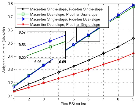
Fig. 3 represents the effect of PBS density on weighted sum rate. The figure shows an increasing trend in the weighted sum rate with the increase in the density of PBSs. This is because of the fact that the increase in PBS density decreases the distances of the users from the PBSs, which decreases the path losses, thus resulting in the improved data rates. The figure shows that the performance of the scheme exploiting dual-slope model in both tiers and the scheme with dual-slope model in pico-tier only is very close. The difference between these schemes is the path loss model in macro-tier whereas, both schemes have dual-slope model in pico-tier. We observe that the effect of dual-slope model on macro-tier is negligible,

Figure 3: Weighted sum rate across varying PBSs density whereas, MBS density is held constant at 1 MBS/sq km.

N = 30,K= 128,Rmin = 4b/s/Hz,rc(macrocell) = 375m, rc(picocell) = 40m andθ1=θ2= 0dB.

20 30 40 50 60 70 80 90 100

0.52 0.54 0.56 0.58 0.6 0.62

Weighted sum rate (Kb/s/Hz)

Critical radius of a Picocell (m)

20 30 40 50 60 70 80 90 1000.65

0.7 0.75 0.8 0.85 0.9

Fraction of users associated to Pico−tier

Macro−tier Single−slope, Pico−tier Dual−slope Macro−tier Dual−slope, Pico−tier Dual−slope Macro−tier Single−slope, Pico−tier Dual−slope Macro−tier Dual−slope, Pico−tier Dual−slope

Figure 4: Weighted sum rate and fraction of users associated to pico-tier across varying critical radius of picocell forN = 25,

M = 6,K = 128,Rmin = 4 b/s/Hz,rc(macrocell) = 375m

andθ1=θ2= 0 dB.

this is mostly due to the fact that the links are long and thus, mostly links are NLoS. This, in turn, makes blocking effect less severe in the macro environment. On the other hand, the effect of dual-slope model in pico-tier is significant due to short link distances. As both schemes have dual-slope model in pico-tier, which dominates the overall behavior due to the higher density of PBSs relative to MBS and thus, both schemes show close performance.

The impact of the critical radius of the picocell on the performance of the network for fixed number of users and BSs is shown in Fig. 4. As the critical radius of the picocell increases, more users start entering within the critical radius, the attenuation decreases due to smaller PLE and the users residing within rc prefer PBSs over MBS. As a result of

2169-3536 (c) 2016 IEEE. Translations and content mining are permitted for academic research only. Personal use is also permitted, but republication/redistribution requires IEEE permission. See

20 30 40 50 60 70 80 90 100

0.2 0.3 0.4 0.5

Weighted sum rate (Kb/s/Hz)

Critical radius of a Picocell (m) Macro−tier Single−slope, Pico−tier Dual−slope

20 30 40 50 60 70 80 90 1000.4

0.6 0.8 1

Fraction of users associated to Pico−tier

Pico−tier PLEs=(2,3) Pico−tier PLEs=(2,4) Pico−tier PLEs=(3,4) Pico−tier PLEs=(2,3) Pico−tier PLEs=(2,4) Pico−tier PLEs=(3,4)

Figure 5: Weighted sum rate and fraction of users associated to pico-tier across varying critical radius of picocell forN = 50,

M = 8, K= 128, Rmin = 4b/s/Hz, rc(macrocell) = 375m

andθ1=θ2= 0dB.

increases with the increase in rc. However, the increasing

trend in the sum rate is sharp in the beginning and then it starts slowing down with further increase in rc. This is

because of the fact that asrc increases, the user offloading to

pico-tier increases but the distance between the PBSs and the users increases and the approximation of LoS links within the critical radius of picocells start affecting. This figure further reveals that the sum rate for the scheme with dual-slope model only in pico-tier is better as more users are offloading from macro-tier and the performance of the network improves. However, after rc = 60 m, the sum rate of the scheme with

dual-slope model in pico tier only decreases as compared to the scheme with dual-slope model in both tiers due to affected link approximation in picocells.

Fig. 5 shows the significance of PLEs of the dual-slope model in a network. This figure assumes dual-slope path loss model in pico-tier and single-slope path loss model in macro-tier. As can be seen from the figure that the case where the PLEs of the pico-tier are smaller, rates are better. This is because the smaller values of PLEs represent less obstruction and attenuation, which decrease the path losses and increase the received power which, in turn, increases the rates. The fraction of users connected with pico-tier is higher for smaller PLEs as they induce reduced attenuation in pico-tier. The figure shows that the worst case happens when both tiers experience approximately same PLEs. This is because the links are approximated using same PLEs in both tiers but both have different critical radii and these PLEs do not perfectly characterize the network, which causes performance degradation.

The user association across varying biasing factor of the pico-tier is plotted in Fig. 6. Biasing effect is investigated by varying the bias factor of the pico-tier,θ2, with no biasing for the macro-tier. An increasing trend in user offloading can be observed with the increasing pico-tier bias factor as biasing improves the received signal strength originating from PBSs. The figure reveals that the biasing with both single and

dual-0 5 10 15 20 25 30

0.4 0.5 0.6 0.7 0.8 0.9 1

Biasing factor of pico−tier, θ₂ (dB)

Fraction of users associated to Pico−tier

Macro−tier Single−slope, Pico−tier Single−slope Macro−tier Dual−slope, Pico−tier Dual−slope Macro−tier Single−slope, Pico−tier Dual−slope Macro−tier Dual−slope, Pico−tier Single−slope

Figure 6: Fraction of users associated with pico-tier across pico-tier biasing factor forN = 25,M = 6,K= 128,Rmin= 4 b/s/Hz, rc(macrocell) = 375 m, rc(picocell) = 60 m and

θ1= 0dB.

0 5 10 15 20 25 30

0.25 0.3 0.35 0.4 0.45 0.5 0.55 0.6 0.65

Biasing factor of pico−tier, θ 2 (dB)

Weighted Sum Rate (Kb/s/Hz) Macro−tier Single−slope, Pico−tier Single−slope Macro−tier Dual−slope, Pico−tier Dual−slope Macro−tier Single−slope, Pico−tier Dual−slope Macro−tier Dual−slope, Pico−tier Single−slope

Figure 7: Weighted sum rate across pico-tier biasing factor for

N = 25,M = 6,K= 128,Rmin = 4b/s/Hz,rc(macrocell) = 375 m,rc(picocell) = 60m and θ1= 0dB.

slope models is beneficial for offloading. However, with dual-slope model in the picocell, this effect is more strong as signal strength from PBSs is further enhanced due to less attenuated links.

0 5 10 15 20 25 30 0

10 20 30 40 50 60 70 80

Biasing factor of pico−tier, θ₂ (dB)

Weighted energy efficiency (b/J/Hz)

Macro−tier Single−slope, Pico−tier Single−slope Macro−tier Dual−slope, Pico−tier Dual−slope Macro−tier Single−slope, Pico−tier Dual−slope Macro−tier Dual−slope, Pico−tier Single−slope

Figure 8: Weighted energy efficiency across pico-tier biasing factor for N = 25, M = 6, K = 128, Rmin = 4 b/s/Hz, rc(macrocell) = 375m, rc(picocell) = 60m and θ1= 0 dB.

0 5 10 15 20

0 2 4 6 8 10 12 14 16

Minimum rate threshold (R_min)

Weighted energy efficiency (Kb/J/Hz)

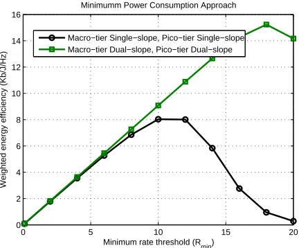
Minimumm Power Consumption Approach

Macro−tier Single−slope, Pico−tier Single−slope Macro−tier Dual−slope, Pico−tier Dual−slope

Figure 9: Weighted EE across varying minimum rate threshold for N = 30, M = 8, K = 128, rc(picocell) = 60 m,

rc(macrocell) = 375m and θ1=θ2= 0dB.

in pico-tier decreases with the increase in the biasing factor. This is due to the fact that as the biasing factor increases, for the fixed number of PBSs, almost all the users offload to pico-tier, however, the power budget at PBS is small compared to MBS, which decreases the received power. This decrease in received power results in decreased data rates. However, with the decrease in power consumption, the weighted energy efficiency shows a huge improvement for these schemes, as shown in Fig. 8.

Furthermore, we investigated the influence of dual-slope path loss model on the HetNet, for weighted EE maximization and power minimization approaches. In Fig. 9, the weighted EE versus minimum rate threshold for the power minimization approach is shown. We compare two different schemes using single-slope and dual-slope path loss models. The sum rate for both schemes is same, i.e.,K×Rmin, fulfilling the minimum

rate requirement of all users. The weighted EE shows an

0 2 4 6 8 10 12 14 16 18

60 80 100 120 140 160 180

Minimum rate threshold (R_min)

Weighted sum rate (b/s/Hz)

EE Maximization Approach

Macro−tier Single−slope, Pico−tier Single−slope Macro−tier Dual−slope, Pico−tier Dual−slope Macro−tier Single−slope, Pico−tier Dual−slope Macro−tier Dual−slope, Pico−tier Single−slope

(a) Weighted sum rate across varying minimum rate threshold

0 2 4 6 8 10 12 14 16 18

0 20 40 60 80 100 120 140

Minimum rate threshold (R_min) Weighted Energy Efficiency (b/J/Hz) Macro−tier Single−slope, Pico−tier Single−slope

Macro−tier Dual−slope, Pico−tier Dual−slope Macro−tier Single−slope, Pico−tier Dual−slope Macro−tier Dual−slope, Pico−tier Single−slope

(b) Weighted EE across varying minimum rate threshold

Figure 10: EE Maximization Approach for N = 30,M = 8,

K = 128, rc(picocell) = 60 m, rc(macrocell) = 375 m and

θ1=θ2= 0 dB.

increasing trend for all schemes in the beginning, as weighted sum rate increases with the increase inRminand then the trend

reverses. This is because the EE is a trade-off between sum rate and power consumption and beyond a certain threshold of Rmin, the effect of power consumption starts dominating

and we observe a decreasing trend in EE. However, the dominating effect of power consumption arrives relatively late when dual-slope model is applied. As dual-slope path loss model better approximates the link compared to single-slope model, the users associate with nearby BSs and experience lower path losses. As a result of lower path losses with dual-slope model, the BSs require less transmit power to fulfill the fixed minimum rate threshold and power consumption is relatively small.

2169-3536 (c) 2016 IEEE. Translations and content mining are permitted for academic research only. Personal use is also permitted, but republication/redistribution requires IEEE permission. See because as the threshold increases, the achievable rate of each

user improves, which increases the overall sum rate. Figure shows that the weighted sum rate is maximum when dual-slope path loss model is applied on pico-tier only as the user offloading is maximum in this case and users connect with the nearby PBSs which decreases the distances between the users and the BSs. This, in turn, increases the rates due to higher received power. When dual-slope model is applied on both tiers, the offloading to the pico-tier is slightly less as compared to the previous mentioned scheme and thus, there is a marginal decrease in sum rate. The offloading to the pico-tier is minimum when the dual-slope model is only applied on the macro-tier as more users prefer MBS over PBSs, thereby triggering the under-utilization of the PBSs and we witness a performance degradation in terms of sum rate in comparison to other schemes.

Fig. 10(b) shows the weighted EE of the system for weighted EE maximization approach. In the start, the scheme with the maximum weighted sum rate shows the maximum weighted EE and the scheme with the minimum weighted sum rate shows the minimum weighted EE. This trend changes at higher values of Rmin. As the minimum rate requirement

increases, the total power consumption increases and we observe a downtrend in EE. This decline in EE comes later for the scheme where dual-slope path loss model is used solely in the network as compared to other schemes. This is mainly due to the fact that the power consumption is less in dual-slope model case due to lower path losses and better approximation of links. Hence, at higher values ofRmin, the EE is maximum

with dual-slope model in both tiers as compared to the case when dual-slope model is observed in pico-tier only.

V. CONCLUSION

In this paper, we analyzed the impact of the dual-slope path loss model on the performance of a downlink HetNet where different PLEs are used for different ranges. In the proposed approach, a joint user association, subcarrier and power allocation is performed to maximize the weighted sum rate. By analyzing the proposed scheme under different path loss models, we observe that the dual-slope model shows significant improvement in data rates and EE in comparison to the single-slope model, which does not measure the PLE dependence on the link distance accurately. The dual-slope path loss model connects the users with the closest BS by offloading them into the minimal attenuation region using smaller PLE. The effect of PLEs were also studied and it has been shown that the users lying within rc undergo lower

path losses with PLE, α0 < 3, in the dual-slope path loss model, as compared to the PLE, α = 3, in the single-slope path loss model. We also observe that the improvement in the performance of the network is significant for rc ≤60m

in picocells due to better LoS links approximation, whereas the effect of the dual-slope model in macro-tier is not very promising. This paper also studied weighted EE maximization and power minimization approaches under dual-slope path loss model. In future, this analysis may be extended to include channel estimation, which will be of significant importance in ultra-dense networks.

APPENDIXA PROOF OFCONVEXITY

Without loss of generality, the objective function in (8) can be written as

f(ρn,m[k], pn,m[k]) =−ρn,m[k]log₂

1 +γn,m[k]pn,m[k]

ρn,m[k]

.

(30)

The gradient of (30) can be calculated as

∇f(ρn,m[k], pn,m[k]) =





1

ln2

h _γ

n,m[k]pn,m[k]

ρn,m[k]+γn,m[k]pn,m[k]

i

−ln

1 +γn,m[k]pn,m[k]

ρn,m[k]

− 1

ln2

_γ

n,m[k]pn,m[k]

ρn,m[k]+γn,m[k]pn,m[k]



.

(31)

The convexity of the objective function in (8) with respect to the optimization variablespn,m[k]andρn,m[k]can be proved by finding the Hessian of f(ρn,m[k], pn,m[k]) as follows

∇2f(ρn,m[k], pn,m[k]) =

γ2_p

n,m[k]

ln2 (ρn,m[k] +γn,m[k]pn,m[k])2

×

" pn,m[k]

ρn,m[k] −1 −1 ρn,m[k]

pn,m[k]

#

.

(32)

Here,ρn,m[k],pn,m[k]andγn,m[k]are the positive val-ues, it can be shown that the eigenvalues are non-negative, thus the Hessian of f(ρn,m[k], pn,m[k]) is positive semi-definite. Therefore, the objective function is proved convex.

APPENDIXB

In case of power minimization approach given the mini-mum rate threshold constraint with equality, i.e.Rn =Rmin,

the achievable rate for user n over all active subcarriers is given as

Rmin=

X

k∈|Kn|

log₂ 1 +γn,m[k]pn,m[k]

. (33)

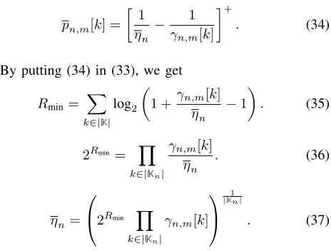
Hence, considering p_n,m[k] ≥ 0, the optimal power allocation, using water filling criteria, is given as

pn,m[k] =

₁

η_n −

1

γn,m[k]

+

. (34)

By putting (34) in (33), we get

Rmin =

X

k∈|K| log₂

1 + γn,m[k]

η_n −1

. (35)

2Rmin ₌ Y

k∈|Kn|

γn,m[k]

η_n . (36)

η_n=



2

Rmin Y

k∈|Kn|

γn,m[k]





1

|Kn|

Hence, the solution to the power minimization problem is given by (26).

APPENDIXC

The weighted energy efficiency (b/J/Hz) can be defined as

EE=

P

m∈M

P

n∈N

P

k∈Kωnrn,m[k]

P

m∈M

P

n∈Nm

P

k∈Kρn,m[k]pn,m[k] +PC

, (38)

whereis the inverse of power amplifier efficiency andPC is

the total circuit power in the network and is defined as

PC=Pcm0+

M−1

X

i=1

Pmi

c . (39)

The optimal transmit power of the BSmover all subcar-riers for an energy efficient system is given as

p∗m=arg max pm∈Pm

φ(pm)

ϕ(pm), (40)

where

Pm=

(

pm∈R:ϕ(pm)≤Pmmax,

X

k∈K

rn,m[k]≥Rmin

)

.

(41)

The function φ(pm)is given by,

φ(pm) =X

n∈N

X

k∈K

ωnρn,m[k]ln

1 + γn,m[k]pn,m[k] Γ

,

(42) whereΓis the SNR gap with respect to the Shannon capacity [42]. Whereas, ϕ(pm)is defined as,

ϕ(pm) =X

n∈N

X

k∈K

ρn,m[k]pn,m[k] +PC. (43)

The optimization problem in (40) can be transformed into an equivalent subtractive objective function and we have

U(η

n) =maxpm

φ(pm)−η

mϕ(pm). (44)

Using (42) and (43), the solution of the optimization problem in (40) can be computed as

∂φ(pm)

∂pn,m[k]

pn,m[k]=p∗_n,m[k]

−η

m

∂ϕ(pm)

∂pn,m[k]

pn,m[k]=p∗_n,m[k]

= 0,∀n, k.

(45)

ωnγn,m[k] Γ

1 +γn,m[k]p∗n,m[k] Γ

−η_m= 0. (46)

Rearranging the above equation, we get

p∗n,m[k] =

"

ωn

η m

− Γ

γn,m[k]

#+

, ∀ k∈K. (47)

After solving (44) and (45) simultaneously and putting

U(η

m) = 0, the optimal water level is given as

−ln(η

m) +ym−

X

n∈N

X

k∈K

ρn,m[k]ωn=η_mxm, (48)

wherexandy are given as

xm=

1

K PC−

X

n∈N

X

k∈K

ρn,m[k]Γ

γn,m[k]

!

. (49)

ym=

1 K

X

n∈N

X

k∈K

ωnln

_ρ

n,m[k]γn,m[k]ωn Γ

. (50)

The closed form of (48) can be obtained by manipulating it with (49) and (50). In order to achieve this, we defineξm= η_mxm, and (48) becomes

ξm=−ln(η_m) +ym−

X

n∈N

X

k∈K

ρn,m[k]ωn. (51)

Rearranging the above equation, we get

η

m=exp{−ξm}.exp

(

ym−

X

n∈N

X

k∈K

ρn,m[k]ωn

)

. (52)

Thus, using (52), (48) can be rewritten as

ξmexp{ξm}=xm.exp

(

ym−

X

n∈N

X

k∈K

ρn,m[k]ωn

)

. (53)

Now, using Lambert functionW(.), we can write

ξm=W

xm.exp

ym−

X

n∈N

X

k∈K

ρn,m[k]ωn

, (54)

η

m=exp

ym−

X

n∈N

X

k∈K

ρn,m[k]ωn

−W xm.exp

ym−

X

n∈N

X

k∈K

ρn,m[k]ωn

.

(55)

REFERENCES

[1] CISCO, “Cisco Visual Networking Index: Global Mobile Data Traffic Forecast Update,” 2013–2018, Feb. 2014.

[2] A. Gupta and R. K. Jha, “A survey of 5G network: Architecture and emerging technologies,”IEEE Access, vol. 3, no. 7, pp.1206-1232, Aug. 2015.

[3] A. Damnjanovic, J. Montojo, Y. Wei, T. Ji, T. Luo, M. Vajapeyam, T. Yoo, O. Song, and D. Malladi, “A survey on 3GPP heterogeneous networks,”IEEE Wireless Commun., vol. 18, no. 3, pp. 10–21, 2011. [4] A. Ghosh, N. Mangalvedhe, R. Ratasuk, B. Mondal, M. Cudak, E.

Visot-sky, T. A. Thomas, J. G. Andrews, P. Xia, H. S. Joet al., “Heterogeneous cellular networks: From theory to practice,”IEEE Commun. Mag., vol. 50, no. 6, pp. 54–64, 2012.

[5] M. R. Mili, and L. Musavian, “Interference Efficiency: A New Metric to Analyze the Performance of Cognitive Radio Networks”,IEEE Trans. Wireless Commun., 2017.

[6] D. Lopez-Perez, I. Guvenc, G. De la Roche, M. Kountouris, T. Q. Quek, and J. Zhang, “Enhanced intercell interference coordination challenges in heterogeneous networks,”IEEE Wireless Commun., vol. 18, no. 3, pp. 22–30, 2011.

2169-3536 (c) 2016 IEEE. Translations and content mining are permitted for academic research only. Personal use is also permitted, but republication/redistribution requires IEEE permission. See

IEEE International Conference on Energy Aware Computing Systems & Applications (ICEAC), pp. 1–4, 2015.

[8] H. Pervaiz, L. Musavian, Q. Ni, “Joint User Association and Energy-Efficient Resource Allocation with Minimum-Rate Constraints in Two-Tier HetNets”,IEEE PIMRC, Sept. 2013.

[9] J. G. Andrews, “Seven ways that HetNets are a cellular paradigm shift,”

IEEE Commun. Mag., vol. 51, no. 3, pp. 136–144, Mar. 2013. [10] S. Corroy, L. Falconetti, and R. Mathar, “Dynamic cell association for

downlink sum rate maximization in multi-cell heterogeneous networks,”

IEEE Int. Conf. on Commun. (ICC), pp. 2457–2461, 2012.

[11] I. Guvenc, “Capacity and fairness analysis of heterogeneous networks with range expansion and interference coordination,” IEEE Commun. Lett., vol. 15, no. 10, pp. 1084–1087, Oct. 2011.

[12] H. Munir, S. Hassan, H. Pervaiz, Q. Ni, L. Musavian, “Energy Efficient Resource Allocation in 5G Hybrid Heterogeneous Networks: A Game Theoretic Approach”,IEEE Veh. Tech. Conf. (VTC), Sept. 2016, Canada. [13] G. Lim, C. Xiong, L. J. Cimini, and G. Y. Li, “Energy-effcient resource allocation for OFDMA-based multi-RAT networks,”IEEE Trans. Wire-less Commun., vol. 13, no. 5, pp. 2696-2705, May 2014.

[14] Z. Wang and W. Zhang, “A separation architecture for achieving energy-efficient cellular networking,”IEEE Trans. Wireless Commun., vol. 13, no. 6, pp. 3113–3123, Jun. 2014.

[15] C. Yang, J. Li, Q. Ni, A. Anpalagan, M. Guizani, “Interference-Aware Energy Efficiency Maximization in 5G Ultra-Dense Networks”,IEEE Trans. on Commun., Vol. 65, Issue 2, pp. 728 -739, Feb. 2017. [16] J. Andrews, S. Singh, Q. Ye, X. Lin, and H. Dhillon, “An overview of

load balancing in HetNets: Old myths and open problems,”IEEE Trans. Wireless Commun., vol. 21, no. 2, pp. 18–25, Apr. 2014

[17] Q. Ye, B. Rong, Y. Chen, M. Al-Shalash, C. Caramanis, and J. Andrews, “User association for load balancing in heterogeneous cellular networks,”

IEEE Trans. Wireless Commun., vol. 12, no. 6, pp. 2706–2716, Jun. 2013. [18] Y. Wang, S. Chen, H. Ji, and H. Zhang, “Load-aware dynamic biasing cell association in small cell networks,”IEEE Int. Conf. on Commun. (ICC), pp. 2684–2689, Jun. 2014,

[19] H. Klessig, M. G¨unzel, and G. Fettweis, “Increasing the capacity of large-scale HetNets through centralized dynamic data offloading,”IEEE 80th Veh. Tech. Conf. (VTC), Sept. 2014.

[20] O. Dousse and P. Thiran, “Connectivity vs capacity in dense ad hoc networks,”IEEE INFOCOM, vol. 1, pp. 476–486, Mar. 2004. [21] J. Liu, M Sheng, L. Liu, and J. Li., “How dense is ultra-dense

for wireless networks: From far-to near-field communications”, IEEE Wireless Commun., Jun. 2016.

[22] J. Liu, W. Xiao, A. C. K. Soong, “Dense Networks of Small Cells”,

Design and Deployment of Small Cell Networks, Cambridge Univ. Press, 2016.

[23] H. Inaltekin, M. Chiang, H. V. Poor, and S. B. Wicker, “On unbounded path-loss models: Effect of singularity on wireless network perfor-mance,”IEEE J. Sel. Areas Commun., vol. 27, no. 7, pp. 1078–1092, Sept. 2009.

[24] X. Zhang and J. Andrews, “Downlink cellular network analysis with multi-slope path loss models,”IEEE Trans. Commun.,vol. 63, no. 5, pp. 1881–1894, May 2015.

[25] M. Ding, P. Wang, D. L´opez-P´erez, G. Mao, and Z. Lin, “Performance impact of LoS and NLoS transmissions in small cell networks,”IEEE Trans. Wireless Commun., Mar 2015.

[26] N. Garg, S. Singh, and J. Andrews, “Impact of dual slope path loss on user association in HetNets”,IEEE Globecom Workshops, pp. 1–6, 2015. [27] J. G. Andrews X. Zhang G. D. Durgin A. K. Gupta, “Are we approaching the limits of wireless network densification?”, IEEE Commun. Mag., 2016.

[28] B. Romanous, N. Bitar, A. Imran, and H. Refai, “Network densifica-tion: Challenges and opportunities in enabling 5G,”IEEE International Workshop on Computer Aided Modelling and Design of Communication Links and Networks (CAMAD), pp. 129–134, 2015.

[29] T. Rappaport, S. Sun, R. Mayzus, H. Zhao, Y. Azar, K. Wang,G. Wong, J. Schulz, M. Samimi, and F. Gutierrez, “Millimeter wave mobile communications for 5G cellular: It will work!”,IEEE Access, vol. 1, pp. 335–349, 2013.

[30] S. Rangan, T. S. Rappaport, and E. Erkip, “Millimeter-wave cellular wireless networks: Potentials and challenges”,IEEE Proc., vol. 102, no. 3, pp. 366–385, Mar. 2014.

[31] J. G. Andrews, T. Bai, M. Kulkarni, A. Alkhateeb, A. Gupta, and R. W. Heath, “Modeling and analyzing millimeter wave cellular systems”,

IEEE Trans. Commun., 2016.

[32] C. B. Andrade and R. P. F. Hoefel, “IEEE 802.11 WLANs: A comparison on indoor coverage models”, IEEE Conf. on Electr. Comput. Eng. (CCECE), pp. 1-6, May 2016.

[33] C. X. Wang, A. Ghazal, B. Ai, Y. Liu, and P. Fan, “Channel mea-surements and models for high-speed train communication systems: A survey”,IEEE Commun. Surveys Tuts., vol. 18, no. 2, pp. 974-987, 2016. [34] T. Bai and R. W. Heath, Jr., “Coverage and rate analysis for millimeter-wave cellular networks”,IEEE Trans. Wireless Commun., vol. 14, no. 2, pp. 1100-14, Feb. 2015.

[35] M. J. Feuerstein, K. L. Blackard, T. S. Rappaport, S. Y. Seidel, and H. Xia, “Path loss, delay spread, and outage models as functions of antenna height for microcellular system design,”IEEE Trans. Veh. Tech., vol. 43, no. 3, pp. 487–498, Aug. 1994.

[36] D. Akerberg, “Properties of a TDMA pico cellular office communication system”,IEEE Veh. Tech. Conf., pp. 186–91, May 1989.

[37] S. Hur et al., “Proposal on mmWave channel modeling for 5G cellular system,”IEEE J. of Sel. Topics Signal Proc., June 2015.

[38] S. Sun et al., “Path loss, shadow fading, and line-of-sight probability models for 5G urban macro-cellular scenarios,”IEEE Global Commun. Conf. (GLOBECOM) Workshop, Dec. 2015.

[39] C . Y. Wong, R. S. Cheng, K. B. Lataief, and R. D. Murch “Multiuser OFDM with adaptive subcarrier, bit, and power allocation,”IEEE J. Sel. Areas Commun., vol. 17, Oct. 1999.

[40] S. Boyd, and L. Vandenberghe,Convex Optimization, Cambridge Uni-versity Press, 2004.

[41] R. Corless, G. Gonnet, D. Hare, D. Jeffrey, and D. Knuth, “On the Lambert W function,”Adv. Comp. Math., vol. 5, pp. 329–359, 1996. [42] J. M. Cioffi, “A multicarrier primer,” Amati Communications