Manuscript version: Author’s Accepted Manuscript
The version presented in WRAP is the author’s accepted manuscript and may differ from the published version or Version of Record.
Persistent WRAP URL:
http://wrap.warwick.ac.uk/132083
How to cite:
Please refer to published version for the most recent bibliographic citation information. If a published version is known of, the repository item page linked to above, will contain details on accessing it.
Copyright and reuse:
The Warwick Research Archive Portal (WRAP) makes this work by researchers of the University of Warwick available open access under the following conditions.
Copyright © and all moral rights to the version of the paper presented here belong to the individual author(s) and/or other copyright owners. To the extent reasonable and
practicable the material made available in WRAP has been checked for eligibility before being made available.
Copies of full items can be used for personal research or study, educational, or not-for-profit purposes without prior permission or charge. Provided that the authors, title and full
bibliographic details are credited, a hyperlink and/or URL is given for the original metadata page and the content is not changed in any way.
Publisher’s statement:
Please refer to the repository item page, publisher’s statement section, for further information.
Model Comparison with Sharpe Ratios
Francisco Barillas, Raymond Kan, Cesare Robotti, and Jay Shanken∗
Abstract
We show how to conduct asymptotically valid tests of model comparison when the extent of
model mispricing is gauged by the squared Sharpe ratio improvement measure. This is equivalent
to ranking models on their squared Sharpe ratios. Mimicking portfolios can be substituted for
any nontraded model factors and estimation error in the portfolio weights is taken into account
in the statistical inference. A variant of the Fama and French (2017) six-factor model, with a
monthly-updated version of the usual value spread, emerges as the dominant model over the period
1972–2015.
∗
1. Introduction
Financial economists have long sought to explain differences in asset expected returns. The
resulting pricing models can be viewed statistically as constrained multivariate linear regressions
of asset returns on systematic factors. The constraint requires that asset expected returns be a
linear function of the betas (the slope coefficients). When returns in excess of a risk-free rate are
employed and the factors are themselves excess portfolio returns or return spreads, the regression
intercepts – the investment alphas – must be zero. The capital asset pricing model (CAPM)
of Sharpe (1964) and Lintner (1965) was the first such model, with the value-weighted market
portfolio of all financial assets serving as the equilibrium-based factor. Equilibrium theory has also
given rise to the intertemporal CAPM of Merton (1973) and Long (1974) and the consumption
CAPM of Breeden (1979) and Rubinstein (1976). These theories motivate the use of state variable
innovations and consumption growth as nontraded asset-pricing factors. However, as Breeden
(1979) notes, maximally-correlated portfolios can also serve as the factors in such models and the
usual asset-pricing restrictions continue to hold.
The empirically motivated three-factor model (FF3) of Fama and French (1993), with traded
size (SMB) and value (HML) factors along with the market excess return (MKT) was, for many
years, the premier factor model in the literature, sometimes supplemented by a momentum factor,
as suggested by Carhart (1997). In recent years, however, the floodgates have opened and many
alternative factor pricing models (to be discussed below) have been explored. In practice, it is
unlikely that a model’s constraints will hold exactly and so it is of interest to quantify the extent
of mispricing for each model. Barillas and Shanken (2017a) address the issue of how to compare
models under the classic Sharpe improvement metric for evaluating the fit of a model. This is the
quadratic form in the alphas that is equivalent to the improvement in the squared Sharpe ratio
(expected excess return over standard deviation) obtained when investment in other asset returns
is permitted in addition to the given model’s factors. This metric is central to the Gibbons, Ross,
and Shanken (GRS, 1989) test of whether a given portfolio is mean-variance efficient, i.e., attains
the maximum possible Sharpe ratio.1
1
A key premise in the analysis of Barillas and Shanken (2017a) is that a model should ideally
price the traded factors in the various models, as well as the returns designated as “test assets.” In
this context, they show thatmodel comparison under the Sharpe improvement metric is driven by
the extent to which each model is able to price the factors in the other models, as reflected in the
“excluded-factor” alphas. Surprisingly, the test assets drop out of the analysis and are, therefore,
irrelevant for model comparison. It follows that the model whose factors permit the highest squared
Sharpe ratio to be achieved is ultimately preferred. The argument is straightforward: for simplicity,
consider two models with traded factors, f1 and f2, respectively. The extent to which f1 fails to
pricef2 and the test-asset returns,R,is measured by the squared Sharpe increase,Sh2(f1, f2, R)−
Sh2(f1), that results from exploiting the corresponding alphas of f2 and R on f1. Similarly,
Sh2(f2, f1, R)−Sh2(f2) indicates the degree of misspecification of the model with factorsf2.Taking the difference givesSh2(f2)−Sh2(f1) and thus the model with “less mispricing” also has the higher squared Sharpe ratio.
Barillas and Shanken (2017a) show that test assets also drop out if models are compared on
the basis of their statistical likelihoods. Barillas and Shanken (2017b) build on this observation
and develop a Bayesian procedure that permits the simultaneous calculation of probabilities for
all models derived from a given set of factors. In essence, their procedure seeks to identify a
par-simonious model that spans the tangency portfolio for the traded factors, but without retaining
redundant factors. Direct evidence about the relative magnitudes of the squared Sharpe ratios for
different models is not provided, however. In this paper, we focus directly on a comparison of
mod-els’ squared Sharpe ratios in an asymptotic analysis under very general distributional assumptions.
Complementary insights about model comparison can thus be obtained by viewing the evidence
from each of these perspectives.
Another criterion for comparison due to Hansen and Jagannathan (HJ, 1997) has frequently
been used in the literature. This “HJ-distance” is a measure of model misspecification that indicates
how closely a proposed stochastic discount factor (SDF) based on a set of factors comes to being
a valid SDF; it can also be regarded as the maximum pricing error of the model over portfolios
with unit second moment. When a risk-free asset is available, Kan and Robotti (2008) suggest
a modification to the HJ-distance which requires that all competing SDFs assign the same price
excessreturns. With traded factors, they further note that imposing the restriction that the factors
are priced without error yields a distance measure equal to the increase in the squared Sharpe ratio.
Thus, our analysis can also be interpreted as a procedure for comparing models in terms of this
modified HJ-distance.
When the factors in one model are all contained in the other – the case of nested models
– the squared Sharpe ratio of the larger model must be at least as high as that for the nested
model. The question then is whether equality holds or the larger model is strictly superior. The
statistical analysis for this scenario is a simple application of the GRS test, with the factors that
are excluded from the nested model serving as left-hand-side returns. The challenge now is to
develop a test for comparing non-nested models, the case in which each model contains factors
not included in the other model. Although the asymptotic distribution of the Sharpe difference
has been derived for a pair of simple trading strategies, the generalization required for model
comparison must accommodate the difference for twotangency portfolios obtained from different
(possibly overlapping) sets of factors.2 We provide such an analysis, while also adjusting for the
well-known small-sample bias in the squared Sharpe ratio estimator, as documented by Jobson and
Korkie (1980). Our simulations indicate that the resulting procedure performs well in samples of
the sort employed in practice.
For models that include nontraded factors, pricing is typically explored using cross-sectional
regression (CSR) analysis. Building on earlier work by Balduzzi and Robotti (2008) and Lewellen,
Nagel, and Shanken (2010), Barillas and Shanken (2017a) note that comparison in terms of a
quadratic form in the generalized least squares (GLS) pricing errors again reduces to examining
the difference of squared Sharpe ratios, but with mimicking portfolios now substituted for the
nontraded factors. In this context, test assets along with any traded factors serve to identify the
mimicking portfolios and the statistical analysis must account for the additional estimation error in
the portfolio weights. We provide asymptotic results for this setting as well. Thus, analyzing models
with nontraded factors again amounts to a comparison of the models’ squared Sharpe ratios – an
intuitively appealing economic criterion. This complements the more statistically-oriented CSR
modelR2s that are often reported and whose asymptotic properties are analyzed by Kan, Robotti,
and Shanken (2013).
2
Our statistical methodology is applied in the comparison of several fairly recent models that
have been explored in the literature. We find that the liquidity-augmented three-factor Fama and
French (1993) model of Pastor and Stambaugh (2003)3 and the “betting-against-beta” CAPM
extension of Frazzini and Pedersen (2014) are dominated by the q-theory model of Hou, Xue, and
Zhang (2015), the Stambaugh and Yuan (2017) mispricing model, and the Fama and French (2017)
five-factor model with cash profitability. A variant of the original Hou, Xue, and Zhang (2015)
model that uses the cash profitability factor instead of its original profitability factor (ROE) is
superior to the six-factor Fama and French (2017) model that also includes momentum. The best
overall performer, however, is a variant of the six-factor Fama and French (2017) model which uses
a “timely” value factor due to Asness and Frazzini (2013) instead of the traditional HML factor.
The rest of the paper is organized as follows. Section 2 presents an asymptotic analysis of
the difference in squared Sharpe ratios for two competing models with traded factors. Section 3
introduces the analysis with nontraded factors, in which case we test the squared Sharpe ratio of
mimicking portfolios. Section 4 introduces a test of multiple model comparison. Section 5 presents
our main empirical findings. Section 6 explores the small-sample properties of the various tests.
Section 7 summarizes our main conclusions. Proofs and additional material are provided in the
Appendix.
2. Comparing Sharpe ratios for models with traded factors
We begin this section with a brief review of the GRS test. First, some definitions and notation.
A factor model M is a multivariate linear regression with N excess returns, R, and K traded
factors, f. WithT observations onft andRt:
Rt=αR+βft+t, t= 1, . . . , T, (1)
whereRt,t, andαR areN-vectors, β is anN ×K matrix, and ft is a K-vector. GRS show that the improvement in the squared Sharpe ratio from adding test assetsRto the investment universe
is a quadratic form in the test-asset alphas:
α0RΣ−1αR=Sh2(f, R)−Sh2(f), (2)
where Σ is the invertible population covariance matrix of the zero-mean disturbance t.4 The
3
This is true with their traded liquidity factor or a mimicking portfolio constructed from their nontraded factor. 4
associated F-statistic is then proportional to the statistic obtained by substituting the sample
quantities in (2) and dividing by one plus the sample estimate ofSh2(f).5 Thus a test ofαR= 0N,
where 0N is anN-vector of zeros, is a test of whetherf yields the maximum squared Sharpe ratio.
Next, we consider pricing restrictions for nested models and show how to implement the GRS
test in this context, with the factors excluded from the nested model serving as left-hand-side
returns.
2.1. Model comparison and alpha-based tests
LetA be a pricing model with factors [f10t, f20t]0 that nests modelB with factorsf1t, wheref1t
and f2t areK1 and K2-vectors, respectively. In addition, letα21 denote the alphas for the factors
f2t when they are regressed on f1t. Proposition 1 in Barillas and Shanken (2017a) shows that to
compare nested models, we need only focus on testing the excluded-factor restriction, α21 = 0K2
(test assets are irrelevant). This restriction can be formally evaluated using the basic alpha test.6
For example, testing the CAPM versus FF3 involves testing whether the CAPM alphas of HML
and SMB are zero. If this joint hypothesis is rejected, we have evidence that FF3 dominates the
CAPM and that the (squared) Sharpe ratio achievable with the factors in FF3 is higher than that
for the market factor. In this case, the tangency portfolio has nonzero weight on HML and/or
SMB.7
Comparing non-nested models is less straightforward, however. For example, let modelAconsist
of MKT and SMB and modelB consist of MKT and HML. Suppose the GRS test indicates that
adding HML increases the squared Sharpe ratio of modelA, while the alpha of SMB on modelB is
not statistically significant. As Barillas and Shanken (2017a) note, such findings would beconsistent
with modelB having the higher squared Sharpe ratio. But in general, failure to reject either model
or finding that both can be rejected does not tell us which model has the higher squared Sharpe
ratio.8 Therefore, in this paper, we develop a direct asymptotic test of this hypothesis.
5
With the usual maximum likelihood estimates, the proportionality constant is (T−N−K)/N and the degrees of freedom of theF distribution areN andT−N−K. The divisor adjusts for the covariance matrix of the alpha estimates conditional on the factorsf.
6
In the empirical section, we employ a version of the test that takes into account residual heteroscedasticity conditional on the factors. We refer to this as the “basic alpha-based test.” This is the special case of Shanken (1990) with no conditioning variables.
7Confidence intervals for the difference of squared Sharpe ratios with nested models can also be obtained as in Lewellen, Nagel, and Shanken (2010).
2.2. Asymptotic distribution of the difference in squared Sharpe ratios for non-nested models
Now consider two non-nested models (A and B) with factor returns fAt and fBt, respectively,
t= 1,2, . . . , T. We assume throughout that all time series are jointly stationary and ergodic with
finite fourth moments. This includes the traded-factor returns and later, nontraded factors and
other basis-asset returns. Denote the maximum squared Sharpe ratios that are attainable from
the two sets of factors by θ2A = µ0AVA−1µA and θB2 = µ0BV
−1
B µB, where µA, µB, VA, and VB are
the nonzero means and invertible covariance matrices of the two sets of factors. Similarly, let the
corresponding sample quantities be ˆθ2A= ˆµ0AVˆA−1µˆA and ˆθB2 = ˆµ0BVˆ
−1 B µˆB.
9
PROPOSITION 1: The asymptotic distribution of the difference in sample squared Sharpe ratios
is given by
√
T([ˆθA2 −θˆB2]−[θA2 −θ2B])∼A N(0, E[d2t]), (3)
provided that E[d2t]>0, where
dt= 2(uAt−uBt)−(u2At−u2Bt) + (θ2A−θ2B), (4)
with uAt=µ0AVA−1(fAt−µA) and uBt=µ0BVB−1(fBt−µB).
Proof: See Appendix.
We prove this result in the Appendix by casting the estimation of the first and second
mo-ments of the returns in the generalized method of momo-ments (GMM) framework and using the delta
method for functions of these parameters. The validity of our asymptotic approximations requires
that at least one of the Sharpe ratios of the models to be compared is different from zero. The
analysis in the Appendix (apart from the proofs of the various lemmas below) accommodates serial
correlation. However, for simplicity, the statements of this and other results in the body of the
paper assume serially uncorrelated time series (factors and returns), a reasonable approximation
for many empirical applications. To conduct statistical tests, we need a consistent estimator of
E[d2t].This can be obtained by replacing each term in dt with the corresponding sample estimate.
We denote the result ˆdt and calculate the sample second moment,
PT
t=1dˆ2t/T.
To better understand the determinants of the asymptotic variance of the difference in sample
squared Sharpe ratios, in the next lemma we assume that the traded-factor returns are multivariate
complicate the interpretation of results. 9
elliptically distributed.
LEMMA 1: When the traded-factor returns are i.i.d. multivariate elliptically distributed with
kur-tosis parameter κ,10 the asymptotic variance of the difference in sample squared Sharpe ratios is
given by
E[d2t] =θA2
4 + (2 + 3κ)θA2
+θ2B
4 + (2 + 3κ)θB2
−2
2ρθAθB[2 + (1 +κ)ρθAθB] +κθ2Aθ2B , (5)
whereρ= Corr[uAt, uBt] =E[uAtuBt]/(θAθB)is the correlation between the returns on the tangency
portfolios of fAt and fBt.
Proof: See Appendix.
The first term is the asymptotic variance of ˆθ2
A, the second term is the asymptotic variance of ˆ
θB2, and the last term is −2 times the asymptotic covariance between ˆθ2A and ˆθB2. The variance of dt depends on ρ, the correlation between the returns on the tangency portfolios of the factors
of models A and B, and on the kurtosis parameter κ. When ρ = 1, that is, the two tangency
portfolios are identical, E[d2t] = 0 and the asymptotic normality result in Proposition 1 breaks
down. When ρ = 0 and the factors are multivariate normally distributed, that is, κ = 0, the
asymptotic variance simplifies to E[d2t] = 2θA2(2 +θ2A) +θ2B(2 +θB2). Finally, it can be shown
thatE[d2t] is an increasing function of the kurtosis parameter κ.
The asymptotic variance in Proposition 1 forms the basis for testing non-nested models. When
the two models have overlapping factors, however, it is important from both an economic and a
statistical perspective to distinguish between two ways the null hypothesis can hold. One possibility
is that the common factors span the (true) tangency portfolio based on the factors from both models.
If so, the squared Sharpe ratio of each model equals that of the common-factors model and the
other factors are redundant. This spanning condition can be evaluated by an alpha-based test,
with the factors that are excluded from each model together serving as the left-hand-side returns.
If spanning is rejected, some or all of the additional factors contribute to an increase in the squared
Sharpe ratio and equality may or may not hold for the two models. In the absence of spanning,
E[d2t]>0 in (4) and one can perform a direct test of θ2A=θ2B using Proposition 1. Alternatively,
given an a priori judgment that exact spanning is implausible and can be ruled out, one can simply
10The kurtosis parameter for an elliptical distribution is defined asκ = µ
use the direct test. In our empirical work, the alpha-based test easily rejects the spanning condition
in all cases considered and so we focus on the direct test in applications.
3. Comparing models with mimicking portfolios
Section 2 dealt with the case in which the factors are excess returns or return spreads. However,
some models, e.g., the consumption CAPM and the intertemporal CAPM, include one or more risk
factors that are not themselves asset returns. Breeden (1979) points out that such factors can be
replaced with portfolios whose weights are proportional to their betas from the projection of the
factors on returns and a constant. In this section, we first present the asymptotic distribution of
the so-called “mimicking portfolio” squared sample Sharpe ratio and then the distribution of the
difference in the sample squared Sharpe ratios for two models that could have as factors mimicking
portfolios.
3.1. Overview of the mimicking portfolio methodology
Suppose that the K-vector ft consists of some traded and some nontraded factors. Let Rt be
a vector of returns that includes the traded-factor returns as well as any basis-asset returns that
will be used to specify mimicking portfolios for the nontraded factors. In a typical cross-sectional
regression analysis, the basis assets would be the “test assets.” For a traded factor, the mimicking
portfolio is, of course, simply the factor itself. As noted by Barillas and Shanken (2017a), in contrast
to the test-asset irrelevance result for traded-factor models, model comparison can depend on the
basis assets used to construct the mimicking portfolios for nontraded factors.11
We define Yt= [ft0, R0t]0 and its population mean and covariance matrix as
µ = E[Yt]≡
"
µf
µR
#
, (6)
V = Var[Yt]≡
"
Vf Vf R
VRf VR
#
. (7)
In the following analysis, we assume thatVf and VR are invertible and thatVRf is of full column
rank.12 Consider the projection of ft on Rt and a constant and denote the resulting
mimicking-11
It should also be noted that increasing the number of basis assets used to construct the mimicking portfolio does not lead, in general, to an increase in the squared Sharpe ratio of the mimicking portfolio returns. A proof of this result is available from the authors upon request.
12
portfolio returns byft∗ =Vf RVR−1Rt≡ARtwithµ
∗=E[f∗
t] =AµRandV∗= Var[ft∗] =AVRA0 =
Vf RVR−1VRf. For the mimicking portfolios to exist, the beta sums must not all be zero, i.e., we
assume that A1N 6= 0K, where 1N is an N-vector of ones and 0K is a K-vector of zeros.13 The population squared Sharpe ratio of a set of mimicking portfolios is given by
θ2=µ∗0V∗−1µ∗ ≡µ0RVR−1VRf(Vf RVR−1VRf)−1Vf RVR−1µR. (8)
Suppose that we have T observations on Yt and let ˆµ and ˆV denote the sample moments of
Yt corresponding to the population moments in (6) and (7). The mimicking portfolio
methodol-ogy estimates the weights of the mimicking portfolios, the matrix A, by running the multivariate
regression
ft=a+ARt+ηt, t= 1, . . . , T. (9)
Let ˆµ∗ = ˆAµˆR and ˆV∗= ˆAVˆRAˆ0, where ˆA= ˆVf RVˆR−1.Then, the sample squared Sharpe ratio of a
set of mimicking portfolios can be obtained as
ˆ
θ2 = ˆµ∗0Vˆ∗−1µˆ∗ ≡µˆ0RAˆ0( ˆAVˆRAˆ0)−1AˆµˆR. (10)
3.2. Asymptotic distribution of the sample squared Sharpe ratio of a set of mimicking portfolios
Letvt=µ0RVR−1(Rt−µR), ut=µ∗0V∗−1(ft∗−µ∗),andyt=µ∗0V∗−1ηt. The following proposition presents a general expression for the asymptotic distribution of ˆθ2.
PROPOSITION 2: The asymptotic distribution of θˆ2 is given by
√
T(ˆθ2−θ2)∼A N(0, E[h2t]), (11)
provided that E[h2t]>0, where
ht= 2ut(1−yt)−u2t + 2ytvt+θ2. (12)
Proof: See Appendix.
When the factors are perfectly tracked by the returns, yt = 0 and the ht expression in the
proposition reduces to
ht= 2ut−u2t+θ2, (13)
13
whereut=µ0fVf−1(ft−µf) and θ2 =µ0fV
−1 f µf.14
To conduct statistical tests, we need a consistent estimator of E[h2t]. This can be obtained by
replacing each term in ht with the corresponding sample estimate. We denote the result ˆht and
calculate the sample second moment,PT
t=1ˆh2t/T.
Additional insight into the determinants of the asymptotic variance of the mimicking portfolio
sample squared Sharpe ratio in Proposition 2 can be obtained by specializing the analysis. The
next result examines the case of factors and returns that are multivariate elliptically distributed.
LEMMA 2: When the factors and returns are i.i.d. multivariate elliptically distributed with kurtosis
parameter κ, the asymptotic variance of θˆ2 is given by
E[h2t] =θ24 + (2 + 3κ)θ2+ 4(1 +κ)E[yt2] θ2R−θ2, (14)
where θ2R =µ0RVR−1µR represents the squared Sharpe ratio of the tangency portfolio of R, E[y2t] =
µ∗0V∗−1Vf·RV∗−1µ∗, and Vf·R = Vf −Vf RVR−1VRf is the covariance matrix of the residuals from projecting the factors on the returns.
Proof: See Appendix.
Note that the first term in (16) is all that would be needed to compute the asymptotic variance
of ˆθ2if the mimicking-portfolio weights were known. The second term in (16) represents the
errors-in-variables (EIV) adjustment required when the weights are estimated. The EIV adjustment term
is nonnegative since 1 +κ >0 andθR2 ≥θ2.15 The latter inequality holds sinceθR2 is the maximum squared Sharpe ratio overall portfolios ofR, whereasθ2 is the maximum squared Sharpe ratio over
combinations of the mimicking portfolios based onR.The impact of the EIV adjustment term on
the asymptotic variance of ˆθ2 can be large when the factors are not well mimicked by the returns,
since in this caseE[y2
t] could be very different from zero.
For example, when K= 1,we have
E[y2t] = (1−R 2)θ2
R2 , (15)
14In this case, the asymptotic approximation provided by Maller, Durand, and Jafarpour (2010) and Maller, Roberts, and Tourky (2016) could be used to derive the asymptotic variance of the sample squared Sharpe ratio. However, from their expression, it is not clear how to accommodate serial correlation, while it is straightforward from inspection of (13).
whereR2=V− 1 2
f Vf RV
−1 R VRfV
−12
f is the coefficient of determination from regressingftonRt. From
this expression, it is clear that there is a negative relationship betweenE[y2
t] andR2,which indicates
thatE[y2t] can be large when the factors are poorly mimicked by the underlying basis-asset returns.
In contrast, when the factors are perfectly tracked by the basis-asset returns, we have E[y2t] = 0
and the EIV adjustment term vanishes.16 The EIV term can also be large whenθR2 −θ2 is positive, that is, when the K-factor pricing model does not hold. Conversely, when the K-factor pricing
holds, i.e., there exists a K-vector λ such that µR = VRfλ, then we have θ2R = θ2, and the EIV
adjustment term will vanish. Finally,E[h2t] is increasing in the kurtosis parameterκ.
3.3. Pairwise model comparison with mimicking portfolios
Nested models. Without loss of generality, assume that modelA hasfAt∗ = [f1∗0t, f2∗0t]0, whereas
model B has fBt∗ = f1∗t. Let µ∗1 = E[f1∗t] and µ∗2 = E[f2∗t]. Similarly, let V11∗ = Var(f1∗t), V12∗ =
Cov(f1∗t, f2∗0t),V22∗ = Var(f2∗t), and V21∗ =V12∗0. Suppose f1∗tis aK1-vector and f2∗tisK2-vector, with
K=K1+K2.
As with traded-factor models, testing the equality of squared Sharpe ratios of mimicking
port-folios when the two models are nested amounts to evaluating the hypothesis that the alphas of
the mimicking portfolios excluded from the smaller model (f2∗t) are zero when regressed on the
mimicking portfolios common to both models (f1∗t). Paralleling the notation in Section 2.1, the
hypothesis isα21∗ = 0K2. In this case, we can no longer use a basic alpha-based test since we have
generated regressors (the portfolio weights).
PROPOSITION 3: Under the null hypothesis H0:α∗21= 0K2,
Tαˆ∗021Vˆ( ˆα∗21)−1αˆ∗21∼Aχ2K2, (16)
where Vˆ( ˆα∗21) is a consistent estimator of
V( ˆα∗21) =E[qtqt0], (17)
with
qt=ξt(1−y1t) +wt(vt−u1t), (18)
16
ξt = (f2∗t −µ∗2)−V21∗V
∗−1 11 (f
∗
1t−µ∗1), y1t = µ∗01V
∗−1
11 (f1t −µ1), η1t = (f1t−µ1) −(f
∗
1t−µ∗1),
η2t= (f2t−µ2)−(f2∗t−µ∗2), u1t=µ∗01V
∗−1 11 (f
∗
1t−µ∗1), and wt=η2t−V21∗V
∗−1 11 η1t.
Proof: See Appendix.
If K2 = 1, we can simply rely on the t-ratio associated with ˆα∗21 to perform the test. In the
traded-factor case, we can employ the basic alpha-based test for the purpose of testing α21= 0K2,
since in this case we have no generated regressors. We also show in the Appendix that the
zero-intercept restriction is equivalent to a restriction in the GLS cross-sectional regression framework,
but with excess returns (the vectorR) projected on covariances with the factors, instead of betas.
Non-nested models. Now consider two non-nested models, A and B, with mimicking portfolios
fAt∗ and fBt∗ , respectively. Let µ∗A = E[fAt∗ ] and µ∗B = E[fBt∗ ]. Similarly, let VA∗ = Var(fAt∗ ) and
VB∗ = Var(fBt∗ ).Finally, denote the nonzero population squared Sharpe ratios that are attainable
from the two sets of mimicking portfolios byθ2
A and θ2B, with sample counterparts ˆθA2 and ˆθ2B.
PROPOSITION 4: The asymptotic distribution of the difference in sample squared Sharpe ratios
is given by
√
T[ˆθ2A−θˆ2B]−[θ2A−θB2]∼A N 0, E[d2t]
, (19)
provided that E[d2t]>0, where
dt=hAt−hBt, (20)
with uAt =µ∗0AVA∗−1(fAt∗ −µ∗A), yAt = µ∗0AVA∗−1ηAt, hAt = 2uAt(1−yAt)−u2At+ 2yAtvt+θA2, and similarly for model B. As defined earlier, ηjt = (fjt−µj)−(fjt∗ −µ∗j) for j=A, B.
Proof: See Appendix.
Proposition 4 reveals that when the factors of models A and B are perfectly spanned by the
basis-asset returns, that is,yAt =yBt= 0,thenE[d2t] collapses to the asymptotic variance provided
in Proposition 1 for the traded-factor case. Typically,yAt and yBt are different from zero, and the
EIV adjustment term can be a main driver of the asymptotic variance of the difference in sample
squared Sharpe ratios of two sets of mimicking-portfolio returns. As earlier, when the factors and
returns are i.i.d. multivariate elliptically distributed, additional insights can be obtained.17 For
example, if the returns on the tangency portfolios of fAt∗ and fBt∗ are perfectly correlated, then
17
Lemma 3 in the Appendix provides an explicit expression forE[d2t] under a multivariate elliptical assumption on
E[d2t] is zero and the asymptotic normality result in Proposition 4 breaks down. Perfect correlation
occurs, in particular, when both modelsAandB price the basis-asset returns correctly so that the
tangency portfolios forA andB both equal the tangency portfolio for the basis-asset returns. This
is unlikely to be true in practice, however.
Similar to the traded-factors scenario, it is important when evaluating two non-nested models
to test whether the common mimicking portfolios (if any) span the tangency portfolio based on the
mimicking portfolios for both models. If so, the mimicking portfolios specific to each model are
redundant and the models deliver the same squared Sharpe ratio. Equivalently, the alphas of those
redundant portfolios must be zero. Testing this hypothesis again boils down to an extension of the
basic alpha-based test to accommodate estimation error in the mimicking portfolio weights – in
this case, with model-specific mimicking portfolios as the left-hand-side returns (see Proposition 5
in the Appendix).
4. Multiple model comparison
Suppose a researcher is considering more than two models and wants to test whether one of the
models – the “benchmark” – is at least as good (it has at least as high squared Sharpe ratio) as
the others. In such a case, the relevant significance level for a series of pairwise comparisons will
not be clear and so a joint test is needed. The analysis with traded factors is outlined here.18 We
begin with the simple case of nested models. Then we turn to the more challenging examination
of non-nested models.
Nested models. Consider a benchmark model that is nested in a series of alternative models. We
form a single alternative model that includes all of the factors contained in the models that nests
the benchmark. It is then easily demonstrated that the expanded model dominates the benchmark
model if and only if one or more of the “larger” models dominates it. Thus, the null hypothesis that
the benchmark model has the same (it cannot be higher) squared Sharpe ratio as these alternatives
can be tested using the methodology developed for pairwise nested-model comparison. Specifically,
we examine the alphas from projecting all the factors excluded from the benchmark model onto
the benchmark factors and test whether these alphas are jointly zero. If we reject the null of zero
alphas, then we conclude that the benchmark model is dominated by one or more of the larger
models. Otherwise, we fail to reject the hypothesis that the benchmark model performs as well as
the other models.
Non-nested models. Our multiple model comparison test for non-nested models is based on the
multivariate inequality test of Wolak (1987, 1989). Suppose we havepmodels. Letδ = (δ2, . . . , δp)
and ˆδ = (ˆδ2, . . . ,δˆp), where δi = θ12−θ2i and ˆδi = ˆθ12−θˆ2i for i = 2, . . . , p. We are interested in testing
H0 :δ ≥0r vs. H1:δ ∈ <r, (21)
where r = p−1 is the number of non-negativity restrictions. Thus, under the null hypothesis, model 1 (the benchmark) performs at least as well as models 2 top(the competing models).
The test is based on the sample counterpart of δ, ˆδ = (ˆδ2, . . . ,δˆp), which has an asymptotic
normal distribution with meanδ and covariance matrix Σδ (conditions for this are provided in the
Online Appendix to Kan, Robotti, and Shanken (2013)). The test statistic is constructed by first
solving the quadratic programming problem
min δ (ˆδ−δ)
0Σˆ−1 ˆ
δ (ˆδ−δ) s.t. δ ≥0r, (22)
where ˆΣδˆis a consistent estimator of Σδ. Let ˜δ be the optimal solution of the problem in (28). The
likelihood ratio test of the null hypothesis is given by
LR=T(ˆδ−δ˜)0Σˆ−ˆ1
δ (ˆδ−δ˜). (23)
A large value of LR suggests that the non-negativity restrictions do not all hold. To conduct
statistical inference, we need the asymptotic distribution of LR. We refer the readers to Kan,
Robotti, and Shanken (2013) for its derivation and a discussion of numerical methods for calculating
the impliedp-value.
In comparing a benchmark model with a set of alternative models, we first remove those
alter-native modelsithat are nested by the benchmark model since by construction the null hypothesis,
δi ≥ 0, holds in this case. If any of the remaining alternatives is nested by another alternative model, we remove the “smaller” model since the squared Sharpe ratio of the “larger” model will
be at least as big. Finally, we also remove from consideration any alternative models that nest
the benchmark, since for nested models the asymptotic normality assumption on ˆδi does not hold
5. Empirical results
We start by describing the factors and the various empirical asset-pricing specifications. Next,
we summarize the empirical findings for the tests of equality of squared Sharpe ratios for competing
traded-factor models. Finally, we explore model comparison for the mimicking-portfolio case.
5.1. Factors and pricing models
We analyze eight asset-pricing models starting with an extension of the Fama-French (1993)
three-factor model which, in addition to the value-weighted market excess return (MKT), the small
minus big (SMB) size factor, and the high minus low book-to-market (HML) value factor, includes
a traded liquidity factor (LIQT) developed by Pastor and Stambaugh (2003) (FF3+LIQT). Second
is the Frazzini and Pedersen (2014) model, which extends the CAPM with the betting-against-beta
factor (BAB) – long low-beta assets and short high-beta assets (MKT+BAB).
The third model is the Fama and French (2017) five-factor model (FF5CP), which adds an
investment factor (CMA) and a cash profitability factor (RMWCP) to the FF3 model. Fama
and French create factors in three different ways. We use what they refer to as their “benchmark”
factors. Similar to the construction of HML, these are based on independent (2×3) sorts, interacting size with cash profitability for the construction of RMWCP, and separately with investments to
create CMA. RMWCP is the average of the two high profitability portfolio returns minus the
average of the two low profitability portfolio returns. Similarly, CMA is the average of the two
low investment portfolio returns minus the average of the two high investment portfolio returns.
Finally, SMB is the average of the returns on the nine small stock portfolios from the three separate
2×3 sorts minus the average of the returns on the nine big-stock portfolios.
Note that FF5CP differs from the original Fama and French (2015) five-factor model which
constructs the profitability factor using anaccruals-based operating profitability measure suggested
by Novy-Marx (2013). Ball et al. (2016) argue that a cash-based measure of profitability yields a
factor that better accounts for average return differences in sorts on accruals. Following Fama and
French (2017), our fourth model adds the up-minus-down (UMD) momentum factor motivated by
the work of Jegadeesh and Titman (1993) to the FF5CP model (FF5CP+UMD).
The fifth model is the Hou, Xue, and Zhang (2015) four-factor model (HXZ), which includes
to Fama and French (2017), HXZ construct their factors from a triple (2×3×3) sort on these characteristics. Moreover, their profitability measure is based on income before extraordinary
items taken from the most recent public quarterly earnings announcement. Our sixth model is
the four-factor model of Stambaugh and Yuan (2015) (SY), which extends the CAPM by adding a
size factor (SMBSY) and two mispricing factors, “management” and “performance” (MGMT and
PERF), that aggregate information across 11 prominent anomalies by averaging rankings within
two clusters exhibiting the greatest return co-movement.
Given that the choice of profitability factor is a key to the performance of the five-factor model
of Fama and French, our seventh model substitutes RMWCP for ROE in the HXZ model (HXZCP).
Our final model (FF5CP*+UMD) includes the more timely value factor HMLm from Asness and
Frazzini (2013) instead of the standard HML. HMLm is based on book-to-market rankings that
use the most recent monthly stock price in the denominator, whereas HML uses annually updated
lagged prices. The sample period for our data is January 1972 to December 2015. Some factors
are available at an earlier date, but the HXZ factors start in January of 1972 due to the limited
coverage of earnings announcement dates and book equity in the Compustat quarterly files.
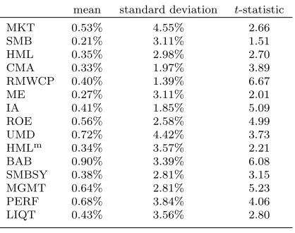
Panel A of Table 1 presents summary statistics for our monthly factor returns – means, standard
deviations, and t-statistics. The latter is, of course, proportional to the factor Sharpe ratio. All
factors have positive and sizable average returns. The factor with the highest return premium is
BAB, followed by UMD, PERF, and MGMT. The size factors, SMB and ME, have the smallest
return premiums. Momentum has the highest volatility of all the non-market factors. All premiums,
with the exception of SMB, havet-statistics larger than 2. The cash profitability factor, RMWCP,
has the lowest standard deviation, which partly explains why it has the highestt-statistic (6.67).
Table 1 about here
Panel B of Table 1 provides the factor correlations. Naturally, different versions of the same
factor tend to be highly correlated. We make a few additional observations about the factors that
are newer to the factor-pricing literature. As noted by Asness and Frazzini (2013), UMD is much
more negatively correlated with timely value, HMLm (−0.654), than with HML (−0.168). On the other hand, correlations between the value, investment, and MGMT factors are strong and positive,
are also high. These mispricing factor correlations make sense insofar as the MGMT cluster includes
the investment/assets anomaly, while the PERF cluster includes momentum and gross profitability.
5.2. Tests of equality of squared Sharpe ratios for competing traded-factor models
In Table 2, we report pairwise tests of equality of the squared Sharpe ratios for different models,
some nested and others non-nested.19 The models are presented from left to right and top to
bottom in order of increasing squared Sharpe ratios. Panel A shows the differences between the
(bias-adjusted) sample squared Sharpe ratios (column model − row model) for various pairs of models. In Panel B, we reportp-values for the tests of equality of the squared Sharpe ratios. The
estimate for each model is modified so as to be unbiased in small samples under joint normality.
This entails multiplying ˆθ2 by (T −K−2)/T and subtractingK/T, eliminating the upward bias, while leaving the asymptotic distribution unchanged. We use * to highlight those cases that are
significant at the 5% level and ** for the 1% level.
Table 2 about here
The diagonal elements of Panel A are the sample squared Sharpe ratio differences between
the model in that column and the next best model.20 As previously discussed, p-values must be
computed differently depending on whether the models to be compared are nested or non-nested.
In the case of nested models, we test whether the factors in the larger model that are excluded from
the smaller model have zero alphas when regressed on the smaller model. For example, since FF5CP
is nested in FF5CP+UMD, the corresponding p-value reported in Panel B is for the intercept in
the regression of UMD on FF5CP.
When the models are non-nested, which is the case for the rest of our comparisons, we use our
19The required condition mentioned earlier, that a model’s Sharpe ratio is nonzero, can be evaluated using a
chi-squared test. Specifically, underH0 :θ2 = 0, Tθˆ2
A
∼χ2K.In our empirical application, we reject this null for all of
our models at the 1% level. In addition, as emphasized by Maller and Turkington (2002), maximizing the squared Sharpe ratio is equivalent to maximizing the ratio itself whenb= 10KV
−1
f µf ≥0.This condition can be tested by
considering ˆb= 10KVˆ
−1
f µˆf and its associated t-statistic. Specifically, the asymptotic distribution of ˆbis given by (a
proof of this result is available from the authors upon request)
√
T(ˆb−b)∼AN(0, E[g2t]),
wheregt=ut(1−yt) +b, ut= 10KV
−1
f (ft−µf),andyt=µ0fV
−1
f (ft−µf).In the data, thebestimates are positive
for all models and the associatedt-ratios range from 4.55 to 9.58, thus suggesting that theb’s for the various models are reliably positive.
20
sequential test. We first check whether the difference in squared Sharpe ratios between the model
composed of the common factors and the one that includes all the factors from both models is
different from zero. This is a test of whether the alphas of the non-common factors on the common
ones are zero. If this test fails to reject, then the evidence is consistent with the common-factors
model being as good as the model that adds the non-overlapping factors. Thus, the two non-nested
models are equivalent as well under this null. However, if the preliminary test rejects, then we
proceed to directly test whether the squared Sharpe ratios of the non-nested models are different
by computing the p-value based on the results in Proposition 1.
For example, in comparing the two non-nested models, HXZ and HXZCP, we first run the
alpha-based test for the different profitability factors, ROE and RMWCP, regressed on the
three-factor model (MKT ME IA) that is nested in these two models. This test easily rejects the joint
hypothesis that both alphas are zero with p-value virtually zero. In fact, this is the case for the
preliminary test in all our non-nested pairwise model comparisons. Had the preliminary test not
rejected in this example, the evidence would be consistent with the three-factor model being as
good as either of the two four-factor models. However, since it did reject, the next step is to divide
the (bias-adjusted) squared Sharpe ratio difference, 0.273−0.166 = 0.107, by its standard error, 0.038, which is the square root of the asymptotic variance given in Proposition 1 divided by the
number of monthly observations (p0.777/528). This yields at-statistic of 2.78, withp-value 0.005,
as reported in Panel B.
The main empirical findings can be summarized as follows. First, the results show that the
FF3+LIQT and MKT+BAB models are outperformed by the other models, with significance at
the 1% level except for HXZ which outperforms MKT+BAB with a 3% level of significance. Next,
FF5CP has a higher sample squared Sharpe ratio than both SY and HXZ, but the difference
between them is not statistically significant. When we add the momentum factor to FF5CP model,
it outperforms HXZ at the 5% level, but it still does not dominate the SY model, which includes
the related factor, PERF. Moreover, adding momentum to FF5CP does not result in a statistically
significant increase in the squared Sharpe ratio. Replacing the original profitability factor (ROE) in
the HXZ model with the cash-based profitability factor (RMWCP) results in a substantial increase
in the squared Sharpe ratio, that is statistically significant at the 1% level. This version of HXZ,
are not reliably different from zero. Finally the choice of value factor in the six-factor Fama and
French (2017) model is important. In fact, with the more timely value factor (HMLm), the model
FF5CP*+UMD outperforms all of the other models at the 5% level.21
Thus far, we have considered comparisons of two competing models. Statistical significance
may be overstated, however, by the inevitable process of “searching” for comparisons that lead to
rejection. Therefore, given a set of models of interest, one may want to test whether a single model,
the “benchmark,” has the highest squared Sharpe ratio of all the models. To explore this issue, we
use the test for non-nested models based on the multivariate inequality analysis of Wolak (1989),
outlined in Section 4. The null hypothesis in this joint test is that none of the other models is
superior to the benchmark. The alternative is that some other model has a higher (population)θ2
than the benchmark.
The empirical results are presented in Table 3. Naturally, since FF5CP*+UMD has the highest
sample squared Sharpe ratio, thep-value for this model in the joint test is very large, consistent with
the conclusion that FF5CP*+UMD performs at least as well in population as the other models.
More interesting is the case in which HXZCP is the benchmark. Whereas FF5CP*+UMD was
superior (p-value of 0.043) to this model in the pairwise comparisons, the p-value for the joint
test with benchmark HXZCP is 0.118. Thus, we miss rejecting the hypothesis that HXZCP has a
squared Sharpe ratio at least as big as those for the alternative models. However, we do continue
to reject the remaining models withp-values close to zero in the joint test except for SY, which we
can only reject at the 5% level.
Table 3 about here
5.3. Model comparison with a nontraded liquidity factor
Section 3 develops a test for comparing competing models when one or both models contain
mimicking portfolios. As an application of that methodology, we explore the nontraded liquidity
factor of Pastor and Stambaugh (2003). Their aggregate liquidity measure is a monthly
cross-sectional average of individual-stock liquidity measures. These individual measures are based on
21
daily returns and volume data and capture the relationship between trading volume and subsequent
returns. The actual series of nontraded factor values, LFt, is then defined in terms of innovations
in aggregate liquidity. The traded factor that we discussed earlier (LIQT) is the value-weighted
return on the 10−1 (high−low) decile portfolio spread from a sort on historical liquidity betas with respect to the nontraded factor LF.
We first construct a mimicking portfolio (LIQM) by regressing LFt on a constant and all of
the traded-factor returns considered above. Thus,R= (MKT, SMB, HML, CMA, RMWCP, ME,
IA, ROE, UMD, HMLm, BAB, SMBSY, MGMT, PERF, LIQT) includes all the factors in the
models that we wish to compare. Additional basis assets could be considered, but are not required.
Although some of these returns are highly correlated, we are interested in the fitted value (the
overall mimicking return), not the individual weights. The sample period is again January 1972 to
December 2015.
There is no requirement for asset pricing or the asymptotic analysis that the mimicking portfolio
be highly correlated with the underlying factors. However, the correlation should be significantly
different from zero so as to avoid complications akin to the “useless factor” problems in
cross-sectional regressions (see Kan and Zhang (1999)). The mimicking portfolio regression for LF has
an adjustedR2of 0.17 and 7 of the 15 mimicking assets have weights that are reliably different from
zero at the 5% level. Furthermore, theFtest of joint significance yields ap-value which is essentially
zero. Thus, the evidence indicates that these asset returns are able to mimic the nontraded factor to
some degree. Surprisingly, the contribution of the traded liquidity factor, LIQT, to the mimicking
portfolio is not reliably different from zero.22
Insofar as marginal utility is low when the market is highly liquid, asset-pricing theory suggests
a positive premium for liquidity risk. The liquidity mimicking portfolio, LIQM, has an average risk
premium of 0.0005 per month over our sample period. The associated t-statistic is 0.27, so the
estimate is not reliably different from zero.23 In contrast, LIQT has an average premium of 0.0043
22Panel B of Table 1 indicates that the correlation between LIQT and the other traded factors is minimal as well. 23
Thet-statistic is computed based on the asymptotic distribution of ˆµ∗, which is given by
√
T(ˆµ∗−µ∗)∼AN(0K, E[qtqt0]), (24)
where
qt= (f
∗
t −µ
∗
) +ηtvt. (25)
or 5.2% annualized, with a t-statistic of 2.80. The correlation between LIQT and LIQM is 0.115,
again not reliably different from zero, whereas the correlation of LIQM with market excess returns
is 0.726.
Although the sample premium for LIQM is not statistically different from zero, the squared
Sharpe ratio for the FF3+LIQM tangency portfolio is positive, as expected, given inclusion of
the FF3 factors.24 Next, we compare the performance of this nontraded liquidity model to that
of the traded-factor models considered earlier, again taking into account estimation error in the
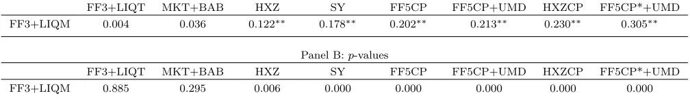
mimicking portfolio weights. Accordingly, Panel A of Table 4 reports the differences in squared
Sharpe ratios. As earlier, models are presented in order of increasing squared Sharpe ratio from
left to right. Finally, we assess the statistical significance of these differences using the result in
Proposition 4, which provides the asymptotic variance of the difference in sample squared Sharpe
ratios for two models with mimicking portfolios. In this application, some terms drop out, since
FF3+LIQM is being compared to models with all traded factors. Panel B of Table 4 reports the
p-values. FF3+LIQM is dominated by all models except for FF3+LIQT and MKT+BAB. Thus,
recalling the evidence in Table 2, neither the traded nor the nontraded liquidity models fare well
in our tests.
Table 4 about here
6. Simulation evidence
In this section, we explore the small-sample properties of our various test statistics via Monte
Carlo simulations. The time-series sample size is taken to be T = 540, close to the actual sample
size of 528 in our empirical work. The factor and basis-asset returns are drawn from a multivariate
normal distribution. We compare actual rejection rates over 100,000 iterations to the nominal 5%
and taking the time-series sample second moment.
24Using a chi-squared test with 4 degrees of freedom we reject the null of a zero squared Sharpe ratio for FF3+LIQM at the 1% level. As for the models with traded factors only, we find no evidence of a negativeb= 10KV∗−1µ∗.It can
be shown that the asymptotic distribution of ˆb= 10KVˆ
∗−1µˆ∗
is given by (a proof of this result is available from the authors upon request and takes into account the estimation error of the weights of the mimicking portfolio)
√
T(ˆb−b)∼AN(0, E[g2t]),
wheregt= 10KV
∗−1 (ft∗−µ
∗
)(1−yt−ut) + 10KV
∗−1
ηt(vt−ut) +b, ut=µ∗0V∗−1(ft∗−µ
∗
),andyt=µ∗0V∗−1ηt.In
level of our tests. A more detailed description of the various simulation designs can be found in
the Appendix.
We start by considering models with traded factors only. As emphasized in Section 2.1, the null
hypothesis of equal squared Sharpe ratios for nested models can be tested using the alpha-based
test. Here, the size of the alpha-based test, with FF3 nested in FF5CP, is inferred from simulations
in which RMWCP and CMA are exactly priced by the three common factors, MKT, SMB, and
HML. The alpha-based test performs very well, with a rejection rate of 5%. Power for the
nested-models test is evaluated by simulating data for which the true squared Sharpe ratios equal the
sample values and thus FF3 is dominated by FF5CP. The rejection rate for this scenario is 100%.
Next, we turn to non-nested models and consider FF3+LIQT vs. HXZCP. This is an example
of non-nested models with a common factor, MKT. In this case, as emphasized in Section 2.2, the
null of equal squared Sharpe ratios can hold when the common factor, MKT, spans the tangency
portfolio based on the factors from both models (SMB, HML, and LIQT for FF3+LIQT, and ME,
RMWCP, and IA for HXZCP). Again, this condition can be tested using the alpha-based test. This
test is right on the money with rejection rates of 5.0% and 100% under the null and alternative
hypotheses, respectively. If we reject this spanning condition, then we can still have equality of
squared Sharpe ratios and this equality can be tested using the normal test in Proposition 1. In this
experiment, the factor means are specified in such a way that the squared Sharpe ratio is the same
for FF3+LIQT and HXZCP, that is, 0.284. The size property of the normal test is excellent (5%).
The power of the normal test is explored using the sample squared Sharpe ratios of FF3+LIQT
and HXZCP as the population squared Sharpe-ratio values. These are 0.058 and 0.284, so the null
hypothesis of equivalent model performance is false in these simulations. The rejection rate of 100%
reflects the large differences in sample squared Sharpe ratios across models and the high precision
of these estimates.
We also examine the small-sample properties of the multiple-comparison inequality test for
non-nested models. Recall that the composite null hypothesis for this test maintains that θ2 for the
benchmark model is at least as high as that for all other models under consideration. Therefore, to
evaluate size, we consider the case in which all models have the sameθ2 value, so as to maximize the
likelihood of rejection under the null. We simulate six different single-factor models corresponding
test withr= 5.Since we calibrate the parameters to the market factor, MKT, the implied common
θ2 for the various models is 0.013. The rejection rates range from 3.3% to 5.9%. Thus, the test
is fairly well specified under the null of equivalent model performance. To examine power, we
simulate four of our original models, FF3+LIQT, HXZ, FF5CP, and FF5CP*+UMD, with the
sample squared Sharpe ratios serving as the populationθ2s. Since FF5CP*+UMD has the highest
θ2, we let each of the remaining models serve as the null model in a multiple comparison test against
three alternative models. Thus, we evaluate power for three different scenarios. The rejection rates
for the test are very high: 100% for FF3+LIQT, 99.9% for FF5CP, and 95.8% for HXZ.
Turning to the analysis with mimicking portfolios, we set R = (MKT, SMB, HML, CMA,
RMWCP, ME, IA, ROE, UMD, HMLm, BAB, SMBSY, MGMT, PERF, LIQT), that is,Rcontains
all the traded-factor returns considered in the empirical section of the paper. We start from the
nested-model case. As emphasized in Section 3.3, this is a situation in which we can no longer
employ the basic alpha-based test to implement nested-model comparison since the mimicking
portfolio weights need to be estimated. Instead, we rely on the chi-squared test in Proposition 3.
The size of this test, with CAPM nested in FF3+LIQM, is inferred from simulations in which the
liquidity mimicking portfolio, SMB, and HML are exactly priced by the common factor, MKT, and
the mean returns, µR,also incorporate the constraint α∗21= 0K2.
Our new test performs very well, with a rejection rate of 5.1%. The power properties of our
chi-squared test are analyzed by simulating data for which the true squared Sharpe ratios equal
the sample values and thus CAPM is dominated by FF3+LIQM (the difference in true squared
Sharpe ratios is 0.041). The rejection rate for this scenario is 100%. If, instead of CAPM nested
in FF3+LIQM, we considered FF3 nested in FF3+LIQM, the power of the test would have been
substantially lower since the difference in true squared Sharpe ratios is only 0.012 in this case.
Naturally, “good” power requires that the differences in model performance are fairly large.
As for non-nested models, we consider FF3+LIQM vs. HXZCP, and test the spanning condition
using our result in Proposition 5 in the Appendix. The chi-squared test enjoys excellent size and
power properties with a rejection rate of 5.3% under the null of spanning and a rejection rate of
100% under the alternative of no spanning. Equality of squared Sharpe ratios can occur also when
the spanning condition is rejected. In this scenario, the normal test in Proposition 4 should be used.
that the squared Sharpe ratio is the same for FF3+LIQM and HXZCP, that is, 0.139. The normal
test is found to perform very well under the null, with a rejection rate of 5.6%. The power of the
normal test is explored using the sample squared Sharpe ratios of FF3+LIQM and HXZCP as the
population squared Sharpe-ratio values. These are 0.054 and 0.284, respectively. The rejection rate
of 98.6% for the normal test is excellent. However, in general, power can be affected by the limited
precision of the sample squared Sharpe ratios of the models, given the residual in the projection of
the nontraded factors on the basis-asset returns.
Finally, in order to analyze the size properties of the multiple-model comparison test, we again
simulate six different single-factor models corresponding to the factors MKT, HMLm, RMWCP,
UMD, IA, and the liquidity mimicking portfolio LIQM. Similar to the traded-factor case, we
cali-brate the parameters to the market factor, MKT. The implied commonθ2 for the various models is
therefore 0.013. The rejection rates range from 3.3% to 5.9%. Thus, the test is fairly well specified
under the null of identical model performance. To examine power, we simulate four of our original
models, FF3+LIQM, FF5CP, HXZ, and FF5CP*+UMD, with the sample squared Sharpe ratios
serving as the populationθ2s. Since FF5CP*+UMD has the highestθ2,we let each of the
remain-ing models serve as the null model in a multiple comparison test against three alternative models.
The rejection rates for the test are 100% for FF3+LIQM, 99.9% for FF5CP, and 96% for HXZ.
In summary, our Monte Carlo simulations suggest that the proposed tests should be fairly
reliable for the sample size encountered in our empirical work.
7. Conclusion
Barillas and Shanken (2017a) analyze model comparison with the extent of model mispricing
measured by the improvement in the squared Sharpe ratio. This is the increase obtained when
investment in other returns (traded factors and test assets) is considered in addition to a model’s
factors. In this framework, model comparison is equivalent to identifying the model whose factors
yield the highest squared Sharpe ratio. Moreover, this result extends to models that include
nontraded factors, with mimicking portfolios substituted for those factors.
We have shown how to conduct asymptotically valid tests for such model comparisons and apply
these methods in an analysis of a variety of factor-pricing models. A variant of the six-factor model
Appendix
Proof of Proposition 2:
The proof relies on the fact that ˆθ2 is a smooth function of ˆµand ˆV. Therefore, once we have
the asymptotic distribution of ˆµ and ˆV, we can use the delta method to obtain the asymptotic
distribution of ˆθ2. Let
ϕ=
"
µ
vec(V)
#
, ϕˆ=
"
ˆ
µ
vec( ˆV)
#
. (A.1)
We first note that ˆµand ˆV can be written as the GMM estimator that uses the moment conditions
E[rt(ϕ)] = 0(N+K)(N+K+1), where
rt(ϕ) =
"
Yt−µ
vec((Yt−µ)(Yt−µ)0−V)
#
. (A.2)
Since this is an exactly identified system of moment conditions, it is straightforward to verify that
under the assumption thatYt is stationary and ergodic with finite fourth moment, we have
√
T( ˆϕ−ϕ)∼A N(0(N+K)(N+K+1), S0), (A.3)
where
S0 =
∞
X
j=−∞
E[rt(ϕ)rt+j(ϕ)0]. (A.4)
Note that S0 is a singular matrix as ˆV is symmetric, so there are redundant elements in ˆϕ. We
could have written ˆϕ as [ˆµ0, vech( ˆV)0]0, but the results are the same under both specifications.
Using the delta method, the asymptotic distribution of ˆθ2 is given by
√
T(ˆθ2−θ2) ∼A N 0,
∂θ2 ∂ϕ0 S0 ∂θ2 ∂ϕ0 0! . (A.5)
It is straightforward to obtain
∂θ2 ∂µ0f = 0
0
K,
∂θ2 ∂µ0R = 2µ
∗0V∗−1A. (A.6)
The derivative ofθ2 with respect to vec(V) is more involved and is given by
∂θ2 ∂vec(V)0 =
00K, µ∗0V∗−1A⊗
00K, −µ∗0V∗−1A
+00K, µ0R VR−1−A0V∗−1A⊗
Using the expression for∂θ2/∂ϕ0, we can simplify the asymptotic variance of ˆθ2 to
V(ˆθ2) =
∞
X
j=−∞
E[ht(ϕ)ht+j(ϕ)], (A.8)
where
ht(ϕ) =
∂θ2 ∂ϕ0rt(ϕ)
= 2µ∗0V∗−1A(Rt−µR) + vec [00K, −µ∗0V∗−1A][(Yt−µ)(Yt−µ)0−V]
"
0K
A0V∗−1µ∗
#!
+ vec [2µ∗0V∗−1, −2µ∗0V∗−1A][(Yt−µ)(Yt−µ)0−V]
"
0K
(VR−1−A0V∗−1A)µR
#!
= 2µ∗0V∗−1(ft∗−µ∗)−µ∗0V∗−1(ft∗−µ∗)(ft∗−µ∗)0V∗−1µ∗
+ 2µ∗0V∗−1(ft−µf)(Rt−µR)0VR−1µR−2µ∗0V∗−1(ft∗−µ
∗
)(Rt−µR)0VR−1µR
−2µ∗0V∗−1(ft−µf)(ft∗−µ∗)0V∗−1µ∗+ 2µ∗0V∗−1(ft∗−µ∗)(ft∗−µ∗)0V∗−1µ∗+θ2
= 2ut−u2t + 2µ∗0V∗−1ηtvt−2µ∗0V∗−1ηtut+θ2
= 2ut(1−µ∗0V∗−1ηt)−u2t + 2µ
∗0
V∗−1ηtvt+θ2
= 2ut(1−yt)−u2t + 2ytvt+θ2. (A.9)
In particular, if ht is uncorrelated over time, then we have V(ˆθ2) = E[h2t], and its consistent
estimator is given by
ˆ
V(ˆθ2) = 1
T
T
X
t=1 ˆ
h2t. (A.10)
When ht is autocorrelated, one can use Newey and West’s (1987) method to obtain a consistent
estimator ofV(ˆθ2).
This completes the proof of Proposition 2.
Proof of Lemma 2
In our proof, we rely on the mixed moments of multivariate elliptical distributions. Lemma 2
of Maruyama and Seo (2003) shows that if (Xi, Xj, Xk, Xl) are jointly multivariate elliptically
distributed and with mean zero, we have
E[XiXjXk] = 0, (A.11)
whereσij = Cov[Xi, Xj]. Consider
ht= 2ut(1−yt)−u2t+ 2ytvt+θ2
from Proposition 2. It is straightforward to show that
E[ut] = 0, (A.13)
E[vt] = 0, (A.14)
E[yt] = 0, (A.15)
E[u2t] =θ2, (A.16)
E[vt2] =θ2R, (A.17)
E[yt2] =µ∗0V∗−1Vf·RV∗−1µ∗, (A.18)
E[utvt] =θ2, (A.19)
E[utyt] = 0, (A.20)
E[vtyt] = 0. (A.21)
With these results and under the multivariate elliptical assumption onYt, we can show that
E[h2t] = 4E[u2t(1−yt)2] +E[u4t] + 4E[yt2vt2]−4E[u3t(1−yt)] + 8E[utvtyt(1−yt)]
−4E[u2tvtyt]−2θ4+θ4
= 4θ2+ 4(1 +κ)θ2E[yt2] + 3(1 +κ)θ4+ 4(1 +κ)θR2E[yt2]−0−8(1 +κ)θ2E[y2t]−0−θ4
= θ2[4 + (2 + 3κ)θ2] + 4(1 +κ)E[y2t](θ2R−θ2). (A.22)
This completes the proof of Lemma 2.
Proofs of Propositions 1 and 4:
Using Proposition 2, we obtain the following expressions for modelsA and B:
hAt =
∂θ2A ∂ϕ
0
rt= 2uAt(1−yAt)−u2At+ 2yAtvt+θA2, (A.23)
hBt =
∂θ2B ∂ϕ
0
rt= 2uBt(1−yBt)−u2Bt+ 2yBtvt+θ2B. (A.24)
By the delta method and equations (A.1)–(A.4), the asymptotic distribution of ˆθ2A−θˆ2Bis given by
√
T([ˆθA2 −θˆB2]−[θA2 −θ2B]) ∼A N 0,
∂(θ2A−θ2B)
∂ϕ
0
S0
∂(θA2 −θB2)
∂ϕ
!
With the analytical expressions of hAt and hBt, the asymptotic variance of
√
T(ˆθA2 −θˆB2) can be written as
∞
X
j=−∞
E[dtdt+j], (A.26)
where
dt=
∂θ2A ∂ϕ −
∂θ2B ∂ϕ
0
rt=hAt−hBt. (A.27)
This completes the proof of Proposition 4.
Note that when the factors are perfectly tracked by the returns, we have that ηjt is a zero
vector and yjt = 0 for j =A, B. Hence, the asymptotic variance in Proposition 4 reduces to that
in Proposition 1 for models with traded factors.
This completes the proof of Proposition 1.
Lemma 3 and Proof of Lemma 1
LEMMA 3: When the factors and returns are i.i.d. multivariate elliptically distributed with kurtosis
parameter κ, the asymptotic variance of the difference in sample squared Sharpe ratios of two sets
of mimicking portfolios,fAt∗ and fBt∗ , is given by
E[d2t] =E[h2At] +E[h2Bt]−2E[hAthBt], (A.28)
with
E[h2At] = θ2A
4 + (2 + 3κ)θA2
+ 4(1 +κ)E[yAt2 ] θ2R−θ2A
, (A.29)
E[h2Bt] = θB2 4 + (2 + 3κ)θ2B+ 4(1 +κ)E[y2Bt] θ2R−θ2B, (A.30)
E[hAthBt] = 2ρθAθB[2 + (1 +κ)ρθAθB] +κθ2Aθ2B
+4(1 +κ)E[yAtyBt](θR2 +ρθAθB−θA2 −θB2), (A.31)
whereρ= Corr[uAt, uBt] =E[uAtuBt]/(θAθB)is the correlation between the returns on the tangency
portfolios of fAt∗ and fBt∗ , E[y2At] =µ∗0AVA∗−1VfA·RVA∗−1µ∗A, E[y2Bt] =µ∗0BV
∗−1 B VfB·RV
∗−1
B µ
∗
B, VfA·R=
VfA−VfARVR−1VRfA, VfB·R=VfB−VfBRVR−1VRfB,andE[yAtyBt] =µ∗0AV
∗−1
A Cov[ηAt, η
0
Bt]V
∗−1
B µ
∗
B.
Proof of Lemma 3: