warwick.ac.uk/lib-publications
A Thesis Submitted for the Degree of PhD at the University of Warwick
Permanent WRAP URL:
http://wrap.warwick.ac.uk/110792
Copyright and reuse:
This thesis is made available online and is protected by original copyright.
Please scroll down to view the document itself.
Please refer to the repository record for this item for information to help you to cite it.
Our policy information is available from the repository home page.
U N
IV ER
SITAS WARWICEN SIS
Source Location Privacy in Wireless Sensor
Networks Under Practical Scenarios: Routing
Protocols, Parameterisations and Trade-Offs
by
Chen Gu
A thesis submitted to The University of Warwick
in partial fulfilment of the requirements
for admission to the degree of
Doctor of Philosophy
Department of Computer Science
The University of Warwick
As wireless sensor networks (WSNs) have been applied across a spectrum of
application domains, source location privacy (SLP) has emerged as a significant
issue, particularly in security-critical situations. In seminal work on SLP, several
protocols were proposed as viable approaches to address the issue of SLP. However,
most state-of-the-art approaches work under specific network assumptions. For
example, phantom routing, one of the most popular routing protocols for SLP,
assumes a single source. On the other hand, in practical scenarios for SLP, this
assumption is not realistic, as there will be multiple data sources. Other issues
of practical interest include network configurations. Thus, thesis addresses the
impact of these practical considerations on SLP. The first step is the evaluation
of phantom routing under various configurations, e.g., multiple sources and
network configurations. The results show that phantom routing does not scale to
handle multiple sources while providing high SLP at the expense of low messages
yield. Thus, an important issue arises as a result of this observation that the
need for a routing protocol that can handle multiple sources. As such, a novel
parametric routing protocol is proposed, called phantom walkabouts, for SLP
for multi-source WSNs. A large-scale experiments are conducted to evaluate
the efficiency of phantom walkabouts. The main observation is that phantom
walkabouts can provide high level of SLP at the expense of energy and/or data
yield. To deal with these trade-offs, a framework that allows reasoning about
trade-offs needs to develop. Thus, a decision theoretic methodology is proposed
that allows reasoning about these trade-offs. The results showcase the viability
First, I would like to express my sincere gratitude to my supervisor Dr. Arshad
Jhumka, whose guidance, encouragement and support have been invaluable to
me during my time in the Department of Computer Science at the University of
Warwick. I benefited greatly from his insightful advice and comments in finding
and solving research problems. Your advice on my research has been priceless. I
look forward to maintaining our collaboration in the future.
I want to thank my fellows in the SLP lab, particularly Matthew Bradbury
and Jack Kirton, who have helped develop me academically and professionally.
Also I would like to thank my lab mates: Dr. Bo Gao, Dr. Huanzhou Zhu,
Dr. Bo Wang, Dr. Chao Chen, Peng Jiang, Dr. Zhuoer Gu, Junyu Li and
Shenyuan Ren, for their stimulating discussions in current technology trends
and for creating all the happy memories that we shared over the last four years.
I would like to thank the staff members in the Department of Computer
Science for giving me tremendous help, both personally and academically over
the past five years. In particular, I thank Dr. Roger Packwood for his support in
solving technical issues and Sharon Howard who solves massive administrative
issues for me.
Last but not the least, I want to express my eternal gratitude to my parents,
who have always given me unconditional love and support through my life. I
would not have undertaken higher education if it were not for my parents, who
This thesis is submitted to the University of Warwick in support of the authors
application for the degree of Doctor of Philosophy. It has been composed by the
author and has not been submitted in any previous application for any degree.
The work presented was carried out by the author except where acknowledged.
For the purpose of reproduction, the source codes of protocols to run simulations
are available at [52] and datasets used to generate results in this thesis can be
found at [53]. More details can be found in the Appendix A.
Parts of this thesis have been previously published by the author in the following:
[54] C. Gu, M. Bradbury, A. Jhumka, and M. Leeke. Assessing the
Perfor-mance of Phantom Routing on Source Location Privacy in Wireless Sensor
Networks. In IEEE 21st Pacific Rim International Symposium on
De-pendable Computing, pages 99–108, 2015. ISBN 9781467393768. doi:
10.1109/PRDC.2015.9. URLhttps://doi.org/10.1109/PRDC.2015.9
[55] C. Gu, M. Bradbury, and A. Jhumka. Phantom walkabouts in
wire-less sensor networks. InProceedings of the ACM Symposium on Applied
Computing, pages 609–616, 2017. doi: 10.1145/3019612.3019732. URL
https://doi.org/10.1145/3019612.3019732
[56] C. Gu, M. Bradbury, J. Kirton, and A. Jhumka. A decision theoretic
framework for selecting source location privacy aware routing protocols
in wireless sensor networks. Future Generation Computer Systems, 2018.
ISSN 0167739X. doi: 10.1016/j.future.2018.01.046. URLhttps://doi.
org/10.1016/j.future.2018.01.046
[82] J. Laikin, M. Bradbury, C. Gu, and M. Leeke. Towards fake sources for
source location privacy in wireless sensor networks with multiple sources.
InIEEE International Conference on Communication Systems, pages 1–6,
2016. doi: 10.1109/ICCS.2016.7833572. URLhttps://doi.org/10.1109/
6LoWPAN IPv6-based Low Power Wireless Personal Area Networks
CEM Cyclic Entrapment Method
CLS Cross Layer Solution
CPM Closest Pattern Matching
CSMA/CA Carrier Sense Multiple Access/Collision Avoidance
CTP Collection Tree Protocol
DAS Data Aggregation Scheme
DBT Dynamic Bidirectional Tree
DCS Data-Centric Sensor Network
DROW Directed Random Walk
DT Decision Theory
FCF Frame Control Field
GPS Global Positioning System
GROW Greedy Random Walk
IEEE Institute of Electrical and Electronics Engineers
ILP Integer Linear Programming
IoT internet of Things
IP Internet Protocol
LPSS Location Privacy Support Scheme
MAC Medium Access Control
NMR Network Mixing Ring
PEM Path Extension Method
PFS Permanent Fake Source
PHR Physical Header
PRESH Probabilistic Reshaping
PW Phantom Walkabouts
RAM Random-access Memory
RF Radio Frequency
RRIN Routing to a Randomly Intermediary Node
RRS Random Routing Scheme
SADRW Self Adjusting Directed Random Walk
SLFSR Short-Lived Fake Source Routing
SLP Source Location Privacy
SPIN Sensor Protocols for Information via Negotiation
STaR Sink Toroidal Region
TDMA Time-Division Multiple Access
TFS Temporary Fake Source
WSN Wireless Sensor Networks
Src The Source node
Sink The Sink node
msg The normal message
Sdir The random walk set of a message
Mdir The random walk direction of a message
Bdir The biased random walk direction of a message
Pbiased The probability of biased random walk
ψ The safety factor
T T The time taken (seconds) of protectionless flooding
Psaf ety The safety period (seconds)
Ms The message with the short random walk
Ml The message with the long random walk
∆ss The distance in hops between the sink and the source
hwalk The remaining hops of the random walk
N C The network configuration
P The name of a given routing protocol
rN C,Pω The result of a attribute underN C andP
RN C,Pω The normalised result of a attribute underN C andP
rN C,P The result vector of all attributes under N C andP
RN C,P The performance vector of all attributes underN C andP
UωN C,P The utility of a single attribute underN C andP
UN C,P The utility of the performance vector underN C andP
ua The aspiration vector
Abstract ii
Acknowledgements iii
Declarations iv
Abbreviations vi
Symbols viii
List of Figures xvi
List of Tables xviii
1 Introduction 1
1.1 Wireless Sensor Networks . . . 2
1.1.1 Overview . . . 2
1.1.2 Components of Nodes . . . 2
1.1.3 Communication Methods . . . 3
1.1.4 Protocol Stack . . . 4
1.1.5 Standardisation . . . 5
1.2 Source Location Privacy in Wireless Sensor Networks . . . 7
1.2.1 Classification of Privacy Issues . . . 7
1.2.2 Why Provide Source Location Privacy? . . . 8
1.2.3 Formalisation of Source Location Privacy Problem . . . . 9
1.3 Problem Statement and Research Contributions . . . 10
1.4 Thesis Organisation . . . 12
2.1.3 Message Structure . . . 17
2.2 Threat Models in Wireless Sensor Networks . . . 18
2.2.1 Adversarial Behaviour . . . 18
2.2.2 View of the Network . . . 20
2.2.3 Resources Strength . . . 21
2.2.4 Network Knowledge . . . 21
2.3 SLP-Aware Routing Protocols in Wireless Sensor Networks . . . 22
2.3.1 Random-Walk Based Techniques . . . 22
2.3.2 Fake-Source Based Techniques . . . 26
2.3.3 Other Techniques . . . 29
2.3.4 Summary of SLP-Aware Routing Protocols . . . 31
2.4 Other Context Privacy Issues . . . 31
2.5 Simulators and Testbeds . . . 34
2.5.1 TOSSIM . . . 34
2.5.2 COOJA . . . 35
2.5.3 RIOT . . . 35
2.5.4 FlockLab . . . 36
2.6 Performance Attributes in Wireless Sensor Networks . . . 37
3 Assessing the Performance of Phantom Routing on Source Lo-cation Privacy in Wireless Sensor Networks 42 3.1 Introduction . . . 42
3.2 Phantom Routing . . . 43
3.2.1 Why Phantom Routing? . . . 43
3.2.2 Phantom Routing Implementation . . . 44
3.3 Problem Statement . . . 46
3.4 Models . . . 46
3.6 Demonstration of Simulation Procedure . . . 52
3.7 Simulation Results . . . 53
3.7.1 Results: Impact of Random Walk Length on SLP . . . 54
3.7.2 Results: Impact of Source Period on SLP . . . 57
3.7.3 Results: Impact of Network Size on SLP . . . 61
3.7.4 Results: Impact of Number of Sources on SLP . . . 66
3.7.5 Results: Other Attributes Discussion . . . 67
3.8 Summary . . . 70
4 Phantom Walkabouts in Wireless Sensor Networks 75 4.1 Introduction . . . 75
4.2 Motivations of Phantom Walkabouts . . . 76
4.2.1 Phantom Routing Review . . . 76
4.2.2 Motivations of Phantom Walkabouts . . . 76
4.3 Implementation of Phantom Walkabouts . . . 79
4.3.1 Random Walk in Phantom Walkabouts . . . 80
4.3.2 Biased Random Walk Routing in Phantom Walkabouts . 83 4.3.3 Phantom Walkabouts . . . 86
4.3.4 Summary: Difference between Phantom Routing and Phan-tom Walkabouts . . . 88
4.4 Problem Statement . . . 90
4.5 Experimental Setup . . . 90
4.6 Simulation Results . . . 91
4.6.1 Baseline: Phantom Routing with Multiple Sources . . . . 91
4.6.2 PW(1,0): SLP with Multiple Sources using Short Random Walks . . . 95
4.6.5 PW(0,1): SLP with Multiple Sources using Long Random
Walks . . . 102
4.7 Discussion . . . 105
4.8 Summary . . . 107
5 A Decision Theoretic Framework for Selecting SLP-Aware Rout-ing Protocols 109 5.1 Introduction . . . 109
5.2 Routing Protocols Review . . . 110
5.2.1 Protectionless Flooding and Protectionless CTP . . . 110
5.2.2 Phantom Routing . . . 110
5.2.3 Phantom Walkabouts . . . 111
5.2.4 DynamicSPR . . . 111
5.2.5 ILP Routing . . . 112
5.3 Decision Theoretic Procedure Overview . . . 112
5.3.1 Introduction to Decision Theory (DT) . . . 113
5.3.2 Decision Theory-Based Heuristic . . . 114
5.4 Decision Theoretic Procedure for Selecting SLP-Aware Routing Protocols . . . 115
5.4.1 Step 1: Profiling and Filtering SLP-Aware Routing Algo-rithms . . . 116
5.4.2 Step 2: Characterisation and Selection of SLP-Aware Rout-ing Algorithms . . . 118
5.5 Problem Statement . . . 119
5.6 An Example: Execution of Decision Theoretic Procedure . . . 119
5.7 Experimental Setup . . . 125
5.8 Case Studies: Routing Protocol Selection for Different Application Scenarios . . . 127
5.8.1 Animal Protection Scenario . . . 129
5.8.2 Asset Monitoring Scenario . . . 131
5.8.3 Military Scenario . . . 134
5.9 Summary . . . 137
6 Conclusions and Further Work 141 6.1 Assessing the Performance of Phantom Routing on Source Loca-tion Privacy under Practical Scenarios . . . 142
6.2 Developing Phantom Walkabouts to Achieve High Level of SLP . 143 6.3 A Decision Theoretic Framework for Selecting SLP-Aware Routing Protocols . . . 143
6.4 Directions for Further Work . . . 144
Bibliography 147
Appendices 173
A Result Reproduction 174
1.1 Demonstration of wireless sensor networks . . . 2
1.2 The components of a sensor node [6] . . . 3
1.3 Classification of privacy issues in the wireless sensor networks . . 7
2.1 TinyOS 2.x header format [121] . . . 18
2.2 The procedures of the hop-by-hop traceback attack . . . 19
2.3 Illustration of phantom routing scheme . . . 23
2.4 Illustration of pure random walk and directed random walk . . . 24
3.1 Illustration of neighbours division in phantom routing. . . 44
3.2 Problem statement: Assessment of phantom routing under
multi-ple sources and various network configurations . . . 47
3.3 Network configurations with multiple sources . . . 48
3.4 Demonstration of messages sent in the safety period . . . 54
3.5 Impact of random walk length: Capture ratio with multiple sources
and network configurations . . . 56
3.6 Impact of random walk length: Receive ratio with multiple sources
and network configurations . . . 57
3.7 Impact of network sizes: Capture ratio with multiple sources and
network configurations when random walk length is 2 hops . . . 59
3.8 Impact of network sizes: Receive ratio with multiple sources and
network configurations when random walk length is 2 hops . . . 60
3.9 Impact of network sizes: Capture ratio with multiple sources and
network configurations when random walk length is 5 hops . . . 62
3.10 Impact of network sizes: Receive ratio with multiple sources and
3.12 Impact of network sizes: Receive ratio with multiple sources and
network configurations when random walk length is 8 hops . . . 65
3.13 Impact of source numbers: Capture ratio with multiple network
sizes and source periods . . . 68
3.14 Impact of source numbers: Receive ratio with multiple network
sizes and source periods . . . 69
3.15 Message latency with multiple sources and network configurations 71
3.16 Messages sent with multiple sources and network configurations . 72
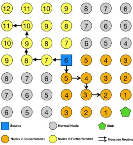
4.1 Illustration of the message routing with short random walks . . . 77
4.2 Illustration of the message routing with short random walks when
an adversary is close to the source . . . 78
4.3 Illustration of the message routing with long random walks . . . 78
4.4 Illustration of neighbours division in phantom routing . . . 80
4.5 Illustration of neighbours division in phantom walkabouts . . . . 81
4.6 Illustration of the routing with random walk in phantom walkabouts 81
4.7 Illustration of bad random walks and biased random walks in the
SourceCorner configuration . . . 84
4.8 Illustration of how the source determines the network configuration
using landmark nodes. Landmark nodes notify ∆n1, ∆n2, ∆n3
to the source by flooding. Then the source knows the network
configuration through Equation 4.2. . . 87
4.9 Problem statement: Evaluation of phantom walkabouts with
various parameterisations . . . 90
4.10 SLP level of protocols for 1, 2 and 3 sources respectively in
SinkCorner configuration . . . 93
4.11 SLP level of protocols for 1, 2 and 3 sources respectively in
4.13 Receive ratio of protocols for 1, 2 and 3 sources respectively in
SourceCorner configuration . . . 98
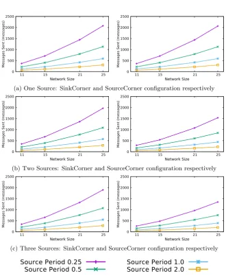
4.14 Messages sent of protocols for 1, 2 and 3 sources respectively in
SinkCorner configuration . . . 100
4.15 Messages sent of protocols for 1, 2 and 3 sources respectively in
SourceCorner configuration . . . 101
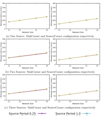
4.16 Message latency of protocols for 1, 2 and 3 sources respectively in
SinkCorner configuration . . . 103
4.17 Message latency of protocols for 1, 2 and 3 sources respectively in
SourceCorner configuration . . . 104
5.1 Problem statement: Selection of the best performing SLP-aware
routing protocol under a practical application . . . 120
5.2 An Example: Protocols results of multiple attributes . . . 121
5.3 An Example: Multiple protocols results of normalised capture
ratio and messages sent . . . 121
5.4 Illustration of the utility functions in the example . . . 124
5.5 Utility of animal protection scenario in SourceCorner configuration132
5.6 Utility of animal protection scenario in SinkCorner configuration 133
5.7 Utility of asset monitoring scenario in SourceCorner configuration 135
5.8 Utility of asset monitoring scenario in SinkCorner configuration . 136
5.9 Utility of military scenario in SourceCorner configuration . . . . 138
5.10 Utility of military scenario in SinkCorner configuration . . . 139
2.1 Summary of SLP-aware routing protocols . . . 32
3.1 Time taken (seconds) of flooding for each network size with one
source . . . 52
3.2 Time taken (seconds) of flooding for each network size with two
sources . . . 52
3.3 Time taken (seconds) of flooding for each network size with three
sources . . . 53
4.1 Commonly used notations . . . 79
4.2 The Difference between phantom routing and phantom walkabouts 89
4.3 Comparison of attributes results under the given network
configu-ration. . . 107
5.1 Commonly used symbols . . . 113
5.2 Time taken (seconds) of flooding for SinkCorner configuration
with various models . . . 126
5.3 Time taken (seconds) of flooding for SourceCorner configuration
with various models . . . 126
5.4 LinkLayer model parameters for the low-asymmetry radio model 127
5.5 Protocols library (L) . . . 129
5.6 Model types of attribute utility funtions . . . 129
5.7 Parameters for attribute utility functions in different scenarios . 129
B.1 The sink-source distance (hops) under the meyer-heavy
communi-cation model and ideal noise model with 1 source . . . 176
B.2 The sink-source distance (hops) under the meyer-heavy
B.4 The sink-source distance (hops) under the casino-lab
communica-tion model and ideal noise model with 1 source . . . 176
B.5 The sink-source distance (hops) under the casino-lab
communica-tion model and low-asymmetry noise model with 1 source . . . . 176
B.6 The sink-source distance (hops) under the meyer-heavy
Introduction
The Internet is rapidly developing which gradually removes the digital barrier
between the Internet and the physical world [123]. In the near future, not only
the computing devices but objects such as cars or even people will be connected to
the Internet. These objects equipped with tiny processors and radio transceivers
known as sensor nodes or motes, can sense different attributes of the environment
and use radio signals to communicate among themselves. The wireless sensor
network (WSN) is one of such technologies and a vital component of the sensing
technology, dealing with vast amounts of information for further processing and
analysis [4]. WSNs have enabled the development of many novel applications [6],
including asset monitoring [5], target tracking [41] and environment control [101]
among others, with low level of intrusiveness. They are also expected to be
deployed in the safety and security-critical systems including military [10] and
medical services [97].
As WSNs have been applied across a spectrum of application domains, they
increase the complexity and challenges in both academia and industry, especially
on data security and privacy. Specifically, the problem of source location privacy
(SLP) has emerged as a significant issue, particularly in security-critical situations.
There is a need to provide SLP because it has been shown that a malicious
attacker can trace the monitored assets by eavesdropping messages in the WSNs.
In many situations, it is very important to hide the physical location of objects
which originally send messages. Mastering the above aspects with the awareness
of the different potential issues becomes one of the most critical research topics
1.1
Wireless Sensor Networks
1.1.1
Overview
WSNs are highly distributed systems consisting of a number of tiny devices,
known as sensor nodes or motes, that can sense physical phenomena and use
radio signals to communicate among themselves (see Figure 1.1). The device
responsible for generating data is called thesource. There is another device called
thesink (or the base station): a powerful device that gathers and processes all the
information collected by the sensor nodes. The sink serves as an interface between
the sensor nodes and the users. Sensor nodes are fitted with a large variety of
physical sensors (e.g., temperature, pressure, humidity and radiation), for the
purpose of monitoring, tracking and controlling environments and assets. In fact,
WSNs have enabled the development of many novel applications in agriculture
and farming [81, 98], environmental monitoring [93, 101, 104], medical services
[27], and military applications [10].
Source nodes
BS
Cloud
Users
Sensor nodes
Figure 1.1: Demonstration of wireless sensor networks
1.1.2
Components of Nodes
The sensor nodes in WSNs normally consist of four essential components [5]:
the sensing unit, the processing unit, the transceiver and the power unit (see
Figure 1.2). The sensing unit consists of a series of physical sensors that
The processing unit is composed of simple 32/64-bit microprocessors which
have limited computational capabilities (typically between 8 and 25 MHz) and
memory space (typically between 4 and 10 kB for RAM). The transceiver (or
radio interface) allows the sensor node to send and receive messages at a low data
rate (between 70 and 250 kB/s) usually in the 2.4 GHz unlicensed industrial,
scientific, and medical (ISM) radio band of the radio spectrum. Choosing between
one band or another depends on the application scenario. Communications in
higher frequency bands have a longer range but find it difficult to overcome
obstacles. Lastly, the power unit provides energy to all the other components to
ensure they operate well. The power unit usually uses two AA batteries (i.e.,
3V) as an energy supply, thus it is regarded as the most limiting component in
sensor nodes as they cannot be replaced or recharged (without other powers that
recycle energy) once the network has been deployed. In addition, sensor nodes
may be equipped with other optional components depending on the practical
scenarios, such as localisation systems (e.g., GPS chips), power scavengers (e.g.,
solar panels) and external flash memories.
Figure 1.2: The components of a sensor node [6]
1.1.3
Communication Methods
In WSNs, data reporting methods could be time-driven, query-driven,
usual one because of energy efficiency. In the event-driven model, a sensor
node starts reporting data to the sink immediately after an event has been
detected (e.g., a sudden change of environment). Instead of establishing a direct
communication link to the sink due to high transmission power consumption,
the source uses multi-hop communications to deliver data which are transmitted
through multiple intermediate nodes. If no events or transmission tasks are
detected, the node becomes inactive (sleep) mode to save energy.
To fulfil these multi-hop communications, there are two basic protocols
adopted to meet the demands of data transmission: flooding and single-path
routing (SPR). Flooding is the simple routing algorithm where the node forwards
data to all its neighbouring nodes except the one that sent it. The intermediate
nodes repeat the process until data visits all the nodes in the network. The
advantage of the flooding protocol is that it is very reliable due to massive data
redundancy. However, it is also very energy inefficient because all the nodes are
involved in transmitting data. On the contrary, the single-path routing protocol
is intended to minimise the number of relaying nodes used to reach the sink. In
the single-path routing, whenever a node has event data to transmit, it sends
the message to a neighbouring node which is closer to the sink than itself. This
operation is repeated for each of the nodes until the data is finally delivered
to the sink. Additionally, some sensor networks may take advantage of
data-aggregation protocols [46, 61, 67, 152] to further reduce network traffic on its
way to the sink. Data aggregation consists of a set of operations (e.g., counting,
average, maximum, minimum) that are performed at some intermediate points
of the network to combine data originating from different sources. Processing
data at intermediate nodes results in more energy-efficient data communication,
thereby increasing the overall lifetime of the network [123].
1.1.4
Protocol Stack
The protocol stack in WSNs has five layers: the physical layer, the data link layer,
layer addresses the needs of simple but robust modulation, transmission, and
receiving techniques. It is responsible for frequency selection, carrier frequency
generation, signal detection, signal processing and data encryption. The data link
layer is responsible for the multiplexing of data streams, data frame detection,
medium access control (MAC) and error control. It ensures reliable
point-to-point and point-to-point-to-multipoint-to-point connections in a communication network. The
network layer takes care of routing the data supplied by the transport layer. It
is responsible for specifying the assignment of addresses and how packets are
forwarded. The transport layer helps to maintain the flow of data if the sensor
networks application requires it. This layer is especially needed when the system
will be accessed through the Internet or other external networks. Depending on
the sensing tasks required, different types of application software can be built
and used on the application layer.
1.1.5
Standardisation
The standardisation has been become a key requirement for the development
of wireless sensor networks. The standards define the functions and protocols
necessary for sensor nodes in the sensor networks [99].
IEEE 802.15.4 Low Rate WPANs
IEEE 802.15.4 is the proposed standard for low rate wireless personal area
networks (LR-WPAN’s) [19, 58]. This standard is designed for wireless sensor
applications that require short-range communication and low power consumption.
IEEE 802.15.4 standard asks devices following the agreed physical and data-link
layer protocols. For instance, the physical layer supports 868/915 MHz low bands
and 2.4 GHz high bands; The MAC layer controls access to the radio channel
using the CSMA/CA mechanism. The IEEE 802.15.4 standard also allows the
formation of the star and peer-to-peer topology for communication between
network devices. In the star topology, the communication is performed between
A network device is either the initiation point or the termination point for
network communications. The PAN coordinator is in charge of managing all
the star PAN functionality. In the peer-to-peer topology, every network device
can communicate with any other within its communication range. The PAN
coordinator acts as the root in the network. The peer-to-peer topology allows
more complex network formations to be implemented such as ad hoc networks.
ZigBee
The ZigBee standard was publicly available in 2005 [92]. It defines the higher layer
(i.e., above network layer) communication protocols upon on the IEEE 802.15.4
standards for LR-PANs. On the physical and data link layer, ZigBee adopts
the IEEE 802.15.4 standard for LR-WPANs. ZigBee also defines mesh, star
and cluster tree network topologies with data security features and application
profiles [99]. ZigBee meets the unique needs of sensors and control devices,
typically with low bandwidth, low latency and very low energy consumption for
long battery lives and for large device arrays.
6LoWPAN
IPv6-based low power wireless personal area networks (6LoWPAN) enables IPv6
packets communication over an IEEE 802.15.4 based network [107]. With the
benefit of the standard, low power devices can communicate directly with IP
devices using IP-based protocols. As the IPv6 packet size is much larger than
the frame size of IEEE 802.15.4, an adaptation layer, new packet format, and
address management are used in the 6LoWPAN standard. 6LoWPAN is designed
1.2
Source Location Privacy in Wireless Sensor
Networks
1.2.1
Classification of Privacy Issues
WSNs have earned acceptance, and extensive work has been done on their
development [28, 57]. However, privacy protection has received a lack of
at-tention, and it is necessary to consider and address all potential privacy risks
that may arise from the adoption of this technology. Threats to privacy in
WSNs can be considered along two dimensions, content privacy and context
privacy (see Figure 1.3) [85]. Content privacy threats relate to use of the content
of the messages broadcast by sensor nodes, such as gaining the ability to read an
encrypted message. Content privacy thus focuses on providing integrity, freshness,
non-repudiation and confidentiality of the messages exchanged in the WSN. In
particular, content privacy includes data aggregation privacy and query privacy.
Data aggregation is designed to substantially reduce the volume of traffic in the
WSN by fusing or compressing data in the intermediate sensor nodes. However,
if intermediate sensor nodes are compromised, an adversary may decrypt the
transmitted data, inject bogus data or tamper with raw data, thus compromising
the content privacy. There are serval techniques for privacy-preserving data
aggregation [59, 119, 158]. In addition, an adversary can also infer client interests
with enquire leak, causing query privacy. Anonymity techniques [20, 157] are
mainly used to address this privacy issue.
Privacy in WSNs
Sink Privacy Source Privacy
Content Privacy Context Privacy
Data Aggregation Privacy Query Privacy Location Privacy Temporal Privacy Other Privacy
On the other hand, context privacy threats focus on the context in which
messages are broadcasted and how information can be observed or inferred by
attackers. Context privacy comprises of hiding the identity, location of nodes and
traffic flow in the WSN. Context is a multi-attribute concept that encompasses
the situational aspects of broadcasted messages, including environmental and
temporal information. Location privacy may arise for such special sensor nodes
such as the source [74, 105, 126, 144, 148] and the sink [32, 33, 72]. It is often
desirable for the source of sensed information to be kept private in the WSN. In
addition, temporal privacy concerns the time when sensitive data is created at
the source, collected by a sensor node and delivered to the sink [75]. This type
of privacy is also very important, because an adversary with knowledge of such
timing information may be able to pinpoint the location of the tracked target
without having the knowledge of data being transmitted in the WSN [75].
1.2.2
Why Provide Source Location Privacy?
For the location privacy, let us use a panda-hunter game [115] as an example.
In a WSN, a node that senses a panda (e.g., temperature changes) informs
the sink that a change has occurred by sending messages that travel through
intermediate nodes to the sink. Poachers attempt to identify the location of the
data source to find the panda. Poachers often with a local vision of network
communications can act in the following way to find the panda: They start
from any point of the network1 and move around. They are equipped with
devices capable of measuring the arrival angle of received signals, which can
estimate the location where the messages sent from. Then poachers move on
to the nodes and repeat the process until they reach the location of panda. As
the movement follows the path of communication, this is usually referred to as
traceback attack. Similar problems occur in other applications. For example,
in a military application, a soldier transmitting messages can unintentionally
1Usually adversaries are assumed to start from the sink, as they can observe any incoming
disclose their location, even when encryption is used. Other real-world examples
include monitoring badgers [41] and the WWF’s Wildlife Crime Technology
Report [1], both of which would likely benefit from context security measures. In
this thesis, the context this thesis focuses on protecting is that ofsource location.
Techniques that protect source location are said to provide source location
privacy (SLP). The SLP problem focuses on ensuring that the location of a source
node or asset can only be observed or inferred by those intended to observe or
decipher it [74]. SLP is important in many application domains, though it is of
utmost concern in security-critical situations. The importance of SLP is not in
the protection of hardware of itself, but the need to hide the presence of events
in the field. In each of these scenarios, it is important to ensure that an attacker
cannot find or deduce the location of the asset being monitored, whether it is
an endangered animal or a soldier. In the panda protection example, poachers
have the local view of the network, meaning that they can monitor a limited
range of messages transmitted. On the other hand, a more powerful adversary
called a global adversary who has a global view of the network uses its sniffers
to eavesdrop all communication. It has been shown that in a non-SLP protected
network, even a weak attacker such as a distributed eavesdropping attacker [71]
can backtrack along message paths through the network to find the source node
and capture the asset [74]. Thus, there is a need to develop SLP-aware routing
protocols.
1.2.3
Formalisation of Source Location Privacy Problem
The SLP problem was first formalised based on the panda-hunter game [74].
In the WSN, the purpose of the network is to monitor the source, while the
purpose of the routing strategy is two-fold, to deliver messages to the sink and
to enhance the location privacy of the asset in the presence of an adversarial
attacker following a movement strategy. This model is formalised containing
six-tuple (G, Sink, Src,P,A,MA), where:
nodes, andEis a set of communication links connecting two distinct nodes.
• Sinkis the network sink, to which all communication in the sensor network
must ultimately be routed to. Typically there is onlyone sink in the WSN.
• Srcis an asset (i.e., the source) that the sensor network monitors.
• P is the routing protocol employed by the sensors to protect the asset from
being acquired or tracked by the attackerA.
• Ais the attacker, or hunter, who seeks to acquire or capture the assetSrc
through a set of movement rulesMA.
The following chapters will expand on this representation and explain aspects
of the panda-hunter game further in the literature. Section 2.1 will detail the
network model includingG,Sinkand Src. The threat model including Aand
MAwill be described in Section 2.2. The routing protocolsP will be reviewed
in Section 2.3.
1.3
Problem Statement and Research
Contribu-tions
Privacy is a key issue in WSNs. Aimed at providing SLP, a number of techniques
have been proposed such as phantom routing using random walks [74, 140],
message delay [64], fake sources [69, 115] and others [31, 113, 124, 127]. Most
existing researchers mainly focus on proposing protocols to provide SLP but are
constrained by a lack of in-depth investigation of SLP in practical scenarios such
as multiple sources and different network configurations.
This thesis aims to handle the SLP issue with multiple sources and different
network configurations. The problem statement is: Could routing protocols
protect SLP under multiple sources and various network
terms of routing protocols, parameterisations and trade-offs. Specifically,
phan-tom routing is evaluated under multiple sources and various configurations.
The results show some shortcomings of phantom routing such as low SLP with
multiple sources. Then a novel parametric routing protocol is proposed, called
phantom walkabouts, for SLP in WSNs. Phantom walkabouts provides high level
of SLP with multiple sources at the expense of data yield. Finally, a decision
theoretic methodology that allows reasoning about these trade-offs is proposed.
This thesis makes the following main contributions:
1. Assessing the performance of phantom routing on source
loca-tion privacy under practical scenarios
In seminal work on SLP, phantom routing was proposed as an approach to
addressing the issue. However, results presented in support of phantom
routing have not included considerations for practical scenarios, omitting
simulations and analyses with multiple sources and different network
con-figurations. These shortcomings above are addressed by conducting an
in-depth investigation of phantom routing under multiple sources and two
different network configurations. Simulations are conducted by varying
four parameters: (i) random walk length, (ii) source period, (iii) network
size and (iv) number of sources. The results demonstrate that previous
work in phantom routing does not provide a high level of SLP with multiple
sources and does not generalise well to different network configurations.
2. Developing phantom walkabouts to achieve high level of SLP
Because recent work has shown some limitations of phantom routing such as
poor performance with multiple sources, phantom walkabouts is proposed,
a novel and more general version of phantom routing, which performs routes
of variable lengths. Phantom walkabouts addresses several shortcomings
of phantom routing such as unexpected termination of the random walk
and poor SLP under a certain network configuration. Parameterisations
performance attributes including receive ratio, messages sent and message
latency. Through extensive simulations, the results show the viability
of phantom walkabouts. For example, under certain parameterisations,
phantom walkabouts achieves extremely high SLP with acceptable decrease
in other attributes.
3. Developing a decision theoretic framework for selecting
SLP-aware routing protocols
Routing protocols such as phantom routing and phantom walkabouts have
been proposed that provide SLP, all of which provide a trade-off between
SLP and other performance attributes. Experiments have been conducted
to gauge the performance of the proposed protocols under different network
parameters such as network sizes. As there exists a plethora of protocols
which contain a set of possibly conflicting performance attributes, it is
difficult to select the SLP protocol that will provide the best trade-offs
across them for a given application with specific requirements. For
ex-ample, the phantom walkabouts provides high level of SLP at expense
of the receive ratio. However, the decrease of the receive ratio may be
not acceptable for some scenario such as military applications. Therefore,
a decision theoretic procedure is proposed for selecting the SLP-aware
routing protocol that achieves the best trade-offs for the applications and
network configurations. The results show the viability of the approach
through different case studies.
More detailed summaries of the contributions are given at the end of Chapter 3,
Chapter 4 and Chapter 5.
1.4
Thesis Organisation
The rest of this thesis is organised as follows.Chapter 2reviews various topics
routing protocols with different techniques, other existing context privacy issues,
simulators and performance attributes.
Chapter 3presents an in-depth investigation of the phantom routing
proto-col under practical scenarios. Phantom routing is implemented with multiple
sources and various network configurations and then assessed by conducting a
range of experiments.
Chapter 4 presents phantom walkabouts, a routing protocol that with
variable random walk lengths. Phantom walkabouts aims to lead an adversary
roaming around in the network, hence keeping the source location safe.
Simu-lations are conducted by varying parameterisations of short and long random
walks in phantom walkabouts, and the results will show better SLP performance
than phantom routing.
InChapter 5, a methodology is proposed where routing protocols are first
profiled to capture their performance according to a desired set of attributes, and
then a decision theoretic procedure is used for selecting the most appropriate
SLP-aware routing protocol for the type of network and application under study.
The results demonstrate the viability of the approach through various case
studies.
Literature Review
As one aim of the thesis is to assess and develop SLP-aware routing protocols,
this chapter first reviews various system models and threat models used in such
protocols in Section 2.1 and Section 2.2. System models investigate the contents
including the sensor nodes, network configurations and the message structure.
For threat models, they focus on the capability of an adversary in WSNs. Under
the definition of system models and threat models, Section 2.3 then explores
some existing methodologies that solve the SLP problem. Some other aspects
of privacy issues in WSNs are also considered as complementary knowledge of
SLP in Section 2.4. Furthermore, Section 2.5 presents popular simulations and
testbeds used to test WSNs. Finally, performance attributes mostly used in
experiments are reviewed in Section 2.6.
2.1
System Models in Wireless Sensor Networks
To investigate the SLP problem, there is a need to specify and model wireless
sensor networks. To present a clear understanding of a network, the system
models are considered from three aspects: (i) sensor nodes, (ii) network and (iii)
the message structure.
2.1.1
Sensor Nodes Modelling
In much of the literature, nodes are randomly deployed in WSNs [25, 29, 42,
94, 122, 136, 138]. They collect data from the environment and send data to
the sink(s). Specifically, when an object appears at a location monitored by a
sensor node, the node becomes the source node and will send messages destined
to report to the sink [72, 129]. When the object moves to a new location, it
may trigger another sensor node to send messages, and that node then becomes
the source [113, 141]. However, some authors assume that the source location
is stationary, i.e., the source does not move in the network [69, 70, 71]. All the
nodes have a limited radio range and nodes within the range can either send or
receive from each other [42, 64, 72, 96, 109, 113, 114]. Because of their limited
radio range, nodes send their data to the sink using multi-hop communication.
Some energy-efficient MAC protocols (e.g., IEEE 802.11) allow nodes to detect
packets while in idle mode [95, 108]. There is only one sink in the network [30, 76],
but it can be either static or mobile [72]. Some authors assume that the sink may
have other capabilities. For instance, the sink knows the network configuration
and is able to monitor the energy consumption and remaining battery power of
every node [141]. In the WSN, nodes know their location and have knowledge of
the location of their adjacent neighbouring nodes through GPS [3, 88, 127, 148].
On the other hand, some authors assume that nodes do not have GPS capability
as localisation services consume too much energy [15, 17, 69, 70, 71]. Instead,
the knowledge of their relative location can be obtained by broadcasting beacon
packets sent from the sink [72].
Nodes in the networks are not only classified into three categories: the source,
normal nodes and the sink [32, 59, 63, 69, 70]. Instead, there are some other
special types of nodes in the networks. Ekici et al. [42] assume that there are
a small number of verifier nodes, which have the responsibility of verifying the
location of sensor nodes and a small number of malicious nodes which possess the
same properties as regular sensor nodes. Another authors [43] assume a hybrid
wireless sensor network with anchor, trusted, and untrusted nodes. Trusted nodes
can utilise standard encryption algorithms to hide an anchor nodes’ positional
information where both anchor nodes and trusted nodes share required common
information. Untrusted nodes use the same radio hardware used by anchor nodes
and trusted nodes. Li et al. [86] assume there is another type of nodes called
do not communicate with each other. They perform random walk movements
on the grid, whereby each transition produces a move of equal probability to a
horizontally or vertically adjacent cell.
2.1.2
Network Modelling
Most authors presume that a WSN is composed of finite two-dimensional grids
(cells) [3, 17, 69, 71, 82, 86, 87, 88, 89, 127, 148]. In the grid network configuration,
Bradbury et al. [17] and Laikin et al. [82] consider theSourceCornerconfiguration
where the single source locates in the corner and the sink is in the centre. Jhumka
et al. [71] consider other configurations called theSinkCorner configuration and
theFurtherSinkCornerconfiguration. In the SinkCorner configuration, the sink is
at the corner of the grid, while the source is at the centre. The FurtherSinkCorner
configuration is similar to the SinkCorner configuration, except that the source
is slightly offset from the centre.
On the other hand, other authors presume a tree configuration that of a
topological tree rooted at the sink [34, 35, 149]. They also presuppose the sink
cannot be compromised and it has a secure mechanism. In a tree communication
model, the root is the sink receiving data from the leaf nodes which simply
act as routers. Besides, Wadaa et al. [136] and Yang et al. [150] assume that
a network is partitioned into a number of clusters through a training process.
In this configuration, a high-end device is deployed into each cluster, acting
as the cluster head. In contrast to sensor nodes, high-end cluster heads have
relatively higher computation capabilities, larger storage sizes, and longer radio
ranges. For the communication in the network, authors [87, 88, 89, 108] assume
bidirectional links only, meaning two nodes are considered neighbours if they
can hear each other and the whole network is fully connected through multi-hop
communications. However, authors [15, 17, 69, 70, 71] do not claim that links
are bidirectional, i.e., links may disappear intermittently.
Authors [69, 70, 134] formalise the network as an undirected graphG= (V, E),
the set of edges E represents the set of links between the nodes. Two nodes
m∈V andm0 ∈V are said to be 1-hop neighbours iff{m, m0} ∈E, i.e.,mand
m0 are in each other’s communication range. The graphG= (V, E) defines the
topology of the network with network of size n×n=N.
2.1.3
Message Structure
For the scope of context privacy, most authors assume that the source encrypts
messages and messages are decrypted at the sink [30, 37, 64, 69, 73, 87, 88]. As
a consequence, the contents of messages will not leak out to prevent an adversary
decrypting or modifying the contents. The encryption procedure can be achieved
by using a shared secret key between the nodes and the sink. However, the
contents of key management [21, 38, 44, 146, 155] including key generation,
distribution and update are beyond the scope of the thesis.
Messages continue to be sent periodically for a certain period, and will stop
when the object leaves the sensor’s monitoring area [72, 113, 129, 141]. They
contain information both in the header and the payload. The header information
is used at every hop for the routing purpose and thus contain information about
the sender and recipient of the message. The payload contains the information
of the monitored object reported by the source. Figure 2.1 is an example of the
CC2420 packet header structure which can be explained as follows [2]: The PHR
contains frame length information; The FCF is the frame control field defined in
the IEEE 802.15.4 specifications and the CC2420 data sheet; The #seqis the
data sequence number, which is incremented for each packet sent by a particular
node. This is used in acknowledging that packet, and also filtering out duplicate
packets; The destination PAN ensures the network can sit side by side with
another TinyOS network and not interfere; The destination is the address of a
packet; The source is the local source ID; The 6LowPAN is the TinyOS network
ID for the 6LowPAN TinyOS Network layer; The AM type defines the type of a
packet.
Figure 2.1: TinyOS 2.x header format [121]
same length [37, 64, 141] and Sheng and Li [128] only consider one-dimensional
data. Each message includes a unique ID where the source event is generated [17,
89, 137]. Therefore, normal nodes can understand whether the messages have
been received and the sink can determine the source node location based on the
ID.
2.2
Threat Models in Wireless Sensor Networks
This section provides an overview of adversarial capabilities that are listed in
several threat models considered in the literature. In particular, this section
reviews the threat models from four aspects of an adversary: (i) adversarial
behaviour, (ii) view of the network, (iii) resources strength and (iv) network
knowledge.
2.2.1
Adversarial Behaviour
An adversarial behaviour could be either active or passive. An active adversary
could use positive behaviour to interfere with traffic flow or communication
behaviours by injecting, modifying or blocking messages [60, 63, 64, 120, 124].
For instance, Shaikh et al. [124] describe how an active adversary uses traffic
analysis attacks to track an asset. Hong et al. [64] describe another active
adversary that is capable of compromising a node to block traffic and to monitor
traffic flow around nodes. He et al. [60] mention data pollution attack where
an adversary tampers with intermediate aggregation results to make the sink
receive the wrong aggregation results.
litera-Source
Normal Nodes
Sink
Attacker
Message
Attacker Movement
Figure 2.2: The procedures of the hop-by-hop traceback attack
ture [3, 29, 40, 45, 65, 72, 109, 116, 127, 130, 151]. A passive adversary does not
actively influence the nodes or the traffic between nodes. Ozturk et al. [116] and
other authors [140, 148] describe a typical behaviour of a passive adversary as
follows. The adversary starts at the location of the sink and only eavesdrops on
the traffic flow between nodes instead of manually changing it. When discovering
an event of a message transmitted in its monitoring area, the adversary uses
an attack strategy that the adversary follows the traffic between the nodes and
traces back in reverse order until reaching the source. This trace strategy is called
a hop-by-hop traceback attack and described in Figure 2.2 and Algorithm 1.
The hop-by-hop traceback attack only monitors traffic flow in the network,
while some other attacks focus on other aspects of the network. Some more
ad-vanced attacks include rate monitoring attack [148], time correlation attack [148]
and timing analysis attack [102]. In the rate monitoring attack, the adversary
monitors nodes with a higher transmission rate, as intuitively these nodes are
probably close to the source or the sink. In the time correlation attack, the
adversary observes the correlation in transmission time between a node and its
neighbour to find the route that a message travels to the sink. Finally, the timing
Algorithm 1A Passive Adversary Strategy: Hop-by-Hop Traceback Attack
1: procedureHop-by-Hop Traceback Attack(sink,source,msg)
2: next location←sink
3: whilenext location6=sourcedo
4: Listen(next location)
5: msg←ReceiveMessage()
6: if IsNewMessage(msg)then
7: next location←CalculateImmediateSender(msg)
8: MoveTo(next location)
9: end if
10: end while
11: end procedure
information, such as the structure of the network and traffic flow [64]. These
advanced attacks may require an adversary having the capability of monitoring
a larger part of the network [37].
2.2.2
View of the Network
There are two types of adversaries when it comes to their network perspectives:
the local and the global adversary. A local adversary has a local view of the
network [32, 124]. Eavesdropping can be achieved using signal detection devices
or other sniffers [65]. For simplicity, authors assume the adversary has a hearing
radius equal to the sensor transmission radius [72, 76, 151]. A local adversary
is sometimes not alone and might collaborate with others. Jhumka et al. [71]
describe a threat model that involves multiple local adversaries collaborating by
sharing information on the configuration and traffic in the WSN. Together these
collaborating adversaries are also regarded as having a multi-local view of the
network. Li and Ren [87] assume that there are some adversaries in the target
area.
On the other hand, a global adversary has a full view of the network [3, 37,
45, 105, 108, 111, 114, 135, 147]. The adversary often uses its own network with
sniffers to eavesdrop on all communications happening in the network. A global
adversary is more powerful than a local adversary due to more knowledge of
network configurations and traffic flow. Normally, SLP solutions that defend
designed against a global adversary can often deal with a local adversary [9].
2.2.3
Resources Strength
A threat model often describes the amount of resources an adversary has in
terms of energy source, memory, move speed and computational capability [36,
87, 124, 127, 132]. The energy source determines whether adversaries can travel
freely in the network. The adversary records data from messages tracking, so
they need memory for data storage. The move speed is often considered with a
passive adversary because passive adversaries often act when hearing message
transmitted. Computational power for an adversary is used to track messages
by calculating the directions of incoming messages or decrypting messages. In
the literature, an adversary is considered as mobile with an unlimited amount of
power [116]. Kamat et al. [74] define the adversary as device rich and resource
rich. Device rich adversaries have the ability to assess the strength of the signal
and determine the angle of arrival of a signal, for example by measuring the
difference in the receiving phase of each element of an antenna array [103].
Meanwhile, resource-rich adversaries can move at any rate and has an unlimited
amount of power. Besides, they also have a large of memory to store information
such as messages that have been received before and nodes they have previously
travelled. Jian et al. [72] also mention that an adversary has memory to remember
his path and performs backtracking.
It is often assumed that strong adversaries have the ability to decrypt the
contents of a message. However, in terms of context privacy, they do not have the
keys to decipher the messages they overhear, so an adversary cannot obtain the
contents of the message [65, 70, 86, 100, 134]. Therefore, some attack strategies
(e.g., clone attack [154]) related to cryptology will not be discussed further.
2.2.4
Network Knowledge
The network knowledge of the adversary varies in the literature. Kamat
sink and algorithms used in the network to protect the panda. Wang et al.
and other authors [76, 110, 131, 140] also assume that the adversary knows the
location of the sink and starts tracking from it. However, Deng et al. [32] assume
that an adversary cannot see the sink visually in a large network. Jhumka
et al. [70] assume that the adversary knows (i) the location of the sink, (ii) the
network configuration and (iii) the routing algorithm. However, the attacker
does not know the number of assets being monitored, and the possible location
of the assets. An attacker also learns about the 1-hop neighbourhood of different
nodes, depending on its location within the network. Besides, the adversary
knows, not only the routing algorithm, but the protection strategy being used in
the network [72, 141].
2.3
SLP-Aware Routing Protocols in Wireless
Sensor Networks
The concept of the SLP problem was first introduced around 2004 [116] which
proposed the panda-hunter game where the poachers only used network traffic
flow to track a panda. Kamat et al. [74] formalise the SLP issue based on the
panda-hunter game. Since then, many techniques have been proposed to address
SLP. The solution spectrum ranges from simple solutions such as pure random
walk [116] to more sophisticated techniques, such as fake sources [17, 71] and
message delay [15, 64]. This section discusses two main categories of solutions:
random-walk based techniques and fake-source based techniques. Other types of
solutions that provide SLP in the literature are also reviewed. For each algorithm,
its theory, strength and weakness will be discussed as well.
2.3.1
Random-Walk Based Techniques
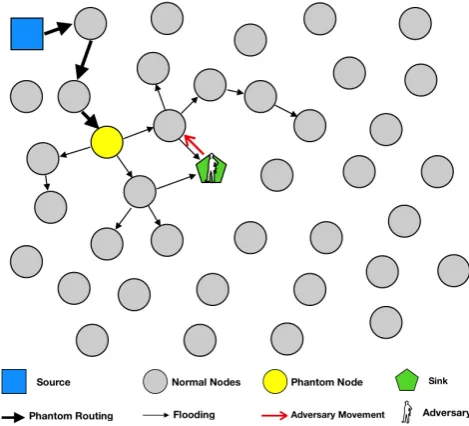
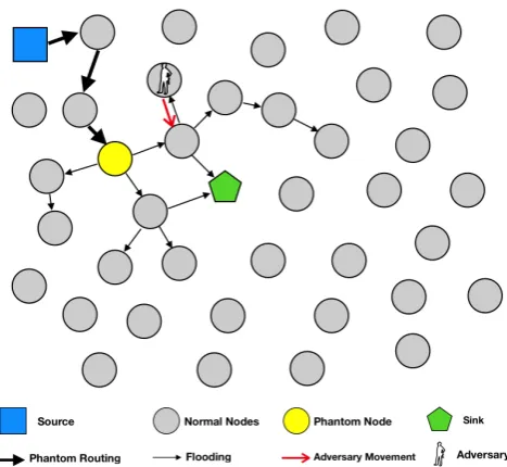
Ozturk et al. [115] use the random walk as a technique to provide SLP. In the
phantom routing scheme (PRS), there are two phases: (i) the random walk phase
Figure 2.3: Illustration of phantom routing scheme
phantom source after travellinghwalkhops, and (ii) a subsequent flooding meant
to deliver messages to the sink (see Figure 2.3). Ozturk et al. discuss the pure
random walk in the phantom routing in detail and claim that the phantom node
is within 20% ofhwalkfrom the real source afterhwalkhops (see Figure 2.4a).
Then Ozturk et al. propose the directed random walk that avoids random walks
cancelling each other out (see Figure 2.4b). Both sector-based directed random
walk and hop-based directed random walk could guarantee phantom sources
far away from the true source. Instead of using flooding for the second phase,
Ozturk et al. also use single path routing algorithms, such as shortest path
routing. The combination of the random walk together with single path routing
is often referred to as the phantom single-path routing scheme (PSRS). Both
PRS and PSRS has received a lot of attention in the literature. On the other
hand, this class of solutions is known to have weaknesses [89, 124, 138], ascribing
poor SLP performance to the directed random walk reusing the routing path and
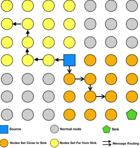
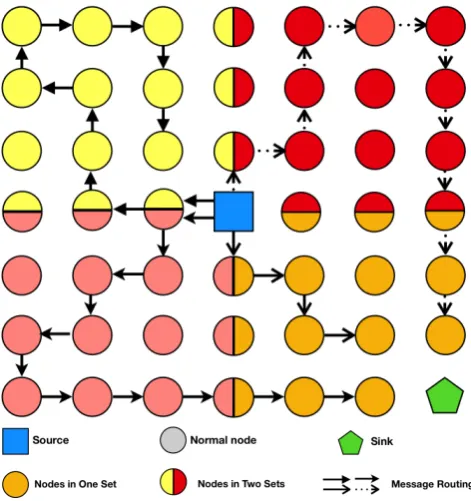
exposing direction information. Zhang [156] introduces an improved algorithm of
a sector-based directed random walk called self-adjusting directed random walk
(a) Pure Random Walk (b) Directed Random Walk
Figure 2.4: Illustration of pure random walk and directed random walk
in SADRW neighbours are divided into four different sets. Nodes randomly pick
a neighbour out of one of the four directional sets and send messages to it. If
an intermediate node receives the message and cannot forward it to the same
direction, then it chooses a new direction to forward the message to until the
message travels a total ofhwalkhops. SADRW solves the weakness of a phantom
walk that may unexpectedly terminate beforehwalkhops, hence increasing the
SLP level.
Wang et al. [140] introduce phantom routing with a locational angle (PRLA).
In PRLA, the random walk is based on the inclination angle between a node and
its neighbours towards the sink. PRLA works as follows. In the deployment stage,
every node calculates the inclination angle between itself and its neighbours.
Then, every node uses the inclination angle to calculate the forward probability
of each of its neighbours. The higher the inclination angle of a neighbour, the
higher the forward probability of that neighbour will be. The source sends
messages to neighbours by using the forward probability of the neighbours. After
the message travelshwalkhops or the last node is not able to forward the message
with the same inclination angle, the message is forwarded to the sink using a
Yao and Wen [151] provide another improvement by introducing the directed
random walk (DROW). In DROW, every node has the knowledge of its own
hop-distance to the sink and the hop-distance of its neighbours to the sink. Each
node chooses the neighbours with a lower hop-distance towards the sink than its
parent’s. When sending messages, the node randomly chooses one of its parents
as the next destination. Authors claim several advantages applying to DROW
such as routing diversity, long safety period1 and energy efficiency. However,
Deng et al. [32] show that DROW does not defend against a time correlation
attack. Wang and Hsiang [139] mention that the direction information retrieved
from the packet headers helps the adversary to find the source of messages.
Xi et al. [144] introduce the greedy random walk (GROW). In the GROW,
one random walk starts from the sink and goes to a randomly chosen
receptor-node. The other random walk starts from the source and meets the first random
walk at the receptor-node. Then the receptor-node uses the path established by
the random walk from the sink to the receptor-node to route the packet from
the source to the sink. In addition, the authors use a different approach, by
recording neighbours in a bloom filter which informs the choice of the next node
to be used in the random walk. However, there is still scope to improve nodes
that are allocated to take part in the directed random walk. Yao and Wen [151]
point out that the random walk used in the GROW is inefficient at creating
a safe distance between the receptor-node and the source. Wang et al. [140]
state that the latency is unstable due to the usage of two random walks. Other
weakness can be found from [89, 122, 124].
An algorithm called randomly selected intermediary node (RRIN) is
intro-duced by Li et al. [88] as an improvement over PRS. Unlike PRS, RRIN does not
leak any directional information via its messages. A source node sends a message
to a chosen intermediate node, and the intermediate node sends the message to
the sink. The choice of the intermediate node must meet the following criteria:
the location of the intermediary node must be at least a minimum distance away
from the source and be normally distributed within the rest of the network.
The authors claim that RRIN has the same latency and power consumption as
PRS, but a higher safety period. Then Li et al. propose a second version of
choosing intermediate nodes. Each node in the WSN has an equal probability
to be the intermediate node of any given source node. The second version of
RRIN consumes much more energy [89] and has a higher delay than PRS, but it
does provide an even better safety period.
There are other algorithms using random walk techniques to address the
SLP issue such as the random routing scheme (RRS) [96], location privacy
support scheme (LPSS) [76] and network mixing ring (NMR) [87]. As random
walk is one of the early techniques used to provide SLP, they could only defend
against a local adversary. In fact, some solutions in the literature have discussed
weaknesses, which shows that the random walk is not always effective. Therefore,
algorithms need to be developed to guard against a powerful adversary with a
global view.
2.3.2
Fake-Source Based Techniques
Algorithms utilise dummy messages sent by afake source to provide SLP. Some
nodes are chosen as fake sources and periodically send dummy messages to
obfuscate the real traffic. In the early stages of this technique, Ozturk et al. [115]
introduce the concept of fake sources and propose a theoretical algorithm called
short-lived fake source routing (SLFSR). The solution works as follows. If a
node receives a real message, it generates a probabilitypto decide whether to
send a dummy message. Ifpis below a thresholdP, then the node broadcasts
a dummy message to all its neighbours. SLFSR consumes more energy but it
could improve the safety period. However, both Kamat et al. [74] and Ozturk
et al. [115] state that only one fake source at the time for only one dummy packet
is not enough to distract an adversary.
Chen and Lou [23] provide two solutions called dynamic bidirectional tree
technique to confuse attackers, in such ways that the attackers are not sure if
they are tracking real traffic from the source, or following dummy traffic. In
DBT, each node knows its distance to the sink and of its neighbours to the
sink. The source randomly sends messages to neighbours with a shorter or equal
hop-distance, which works similar to the first stage of phantom routing. Then
intermediary nodes use a probability pto randomly select a neighbour to create
a branch and forward dummy traffic for h hops. The second solution (ZBT)
makes messages walk zigzags in the network. Firstly the sink generates one
proxy sink with each of its sides. Then the source randomly selects a node as a
proxy source which isihops away from itself. The real traffic is following the
route that messages are from the source, to the proxy source, to the proxy sink,
and finally to the sink.
Jhumka et al. [71] propose another algorithm. Jhumka et al. first prove the
fake sources selection problem to be NP-complete and the algorithm works as
follows. The source node sends a normal message to the sink. When the sink
receives it, it waits a short period and broadcastshawayimessages that floods
the network. When a 1-hop neighbour of the sink receives thehawayimessage
it becomes a temporary fake source (TFS) and broadcasts hf akei messages
for a period. Before the TFS becomes a normal node they broadcast hchoosei
messages. When a normal node receives the hchoosei message it becomes a
permanent fake source (PFS) if the node believes itself to be the furthest node
in the network from the sink, otherwise it will become a TFS.
Bradbury et al. [17] improve the algorithm in [71] through the online
esti-mation of its parameters. As the consequence, the improved algorithm provides
a better SLP level than [71] without requiring prior network knowledge. Then
Bradbury et al. propose DynamicSPR which is an extended version of the
dy-namic fake source technique [17]. Dydy-namicSPR optimises the way fake sources
are allocated, in such a way that fake sources perform a directed random walk
away from the sink. This algorithm reduces the number of fake sources present in