Design of Photovoltaic System using Fuzzy Logic Controller

© 2019, IRJET | Impact Factor value: 7.211 | ISO 9001:2008 Certified Journal

| Page 1400

Design of Photovoltaic System using Fuzzy Logic Controller

M. Khallaf

_{, A. Ismail}

1

_{Graduate Student, Dept. of Electrical Engineering, Rochester Institute of Technology, Dubai, UAE}

2

_{Professor, Dept. of Electrical Engineering, Rochester Institute of Technology, Dubai, UAE}

---***---Abstract -

Controller in a standalone Photovoltaic (PV) system. The PV system was designed and simulated using MATLAB/Simulink where an array of Sun Power SPR-440NE-WHT-D solar panels was connected to a boost DC-DC converter. The number of parallel strings along with the number of series modules in each string of the PV panel have been designed to produce an output power of 150 KW at standard testing conditions (STC). The controller was assessed in terms of dynamic response, output power efficiency, and output ripples. These variables were tested under two scenarios; the first under fixed weather conditions and the second under varying weather conditions.

Key Words: Renewable Energy, PV, MPPT, and Fuzzy Logic

1. INTRODUCTION TO FUZZY LOGIC

Fuzzy logic is considered a type of many-valued logic (MVL) otherwise called non-classical logic. They are a form of logic that do not constrain the output truth-values to only two but accept the range of values in between as well [1]. This means that it is not restricted to binary values of “0” and “1” or “True” and “False”, but operates as well in the grey area in between allowing for a more accurate indication of the variable. Another unique attribute that fuzzy logic has is the use of linguistic interpretation instead of numerical, which makes it closer to the human thought process. When Lukasiewicz and Tarski introduced infinite-valued logic in 1920 and when Lotfi Zadeh perfected it and introduced fuzzy Logic in 1965, the aim was to create a new framework that is not only black and white [2].

1.1 FUZZY SETS AND MEMBERSHIP FUNCTIONS

Fuzzy logic is a unique method that transforms mathematical equations into a set of linguistic commands which is done using two crucial concepts: fuzzy sets and membership functions. Fuzzy sets are a group of sets where the numerical data gets allocated to, and by doing so it transforms numerical values into linguistic ones. Fuzzy sets are similar to the Mathematical concept of having a universe of discourse, where a universe defined as Z contains all the values and the data are grouped. A simple example of a fuzzy set would be creating three sets called low, medium, and high, used to divide and group the available numerical data into these sets using the second concept, which is the membership function. The membership function is a tool developed through the experience of the user and is used to assess the degree to which this value belongs to a certain set and is evaluated on a

scale of zero to one. As shown in Figure 1, the triangle shape represents the membership function which is bound by zero and one, where zero means that the variable does not belong to the set at all and one means that it the variable entirely belongs to the set.

Fig -1 Membership Function Diagram [3]

1.2 FUZZY RULES AND REASONING

A fuzzy set can be adapted and tailored towards any application and that is due to the fuzzy rules that are embedded in each of the sets. A fuzzy rule is a statement developed by the user of the logic based on the knowledge of the industry experts to determine the output based on the input variables. These rules are formulated as conditional statements that utilize the “if” and “then” arguments along with some logic gates as well such as “and”, “not” and “or” [4]. The rules were built in such a way to mimic the day-to-day human reasoning that is being done naturally such as “IF room temperature is low THEN switch the air-conditioning to low.” In this conditioning statement, the “if” and “then” argument was used to figure out the output and input. In this case, the output is the air-conditioning fan level and the input is the room temperature. The final elements of the rule are the fuzzy sets that represent both the input and the output values, which in this case are both called low. A general fuzzy rule should look like Equation 1:

IF X is FS THEN Y is FS (1) Where:

X is the input measured variable.

© 2019, IRJET | Impact Factor value: 7.211 | ISO 9001:2008 Certified Journal

| Page 1401

fuzzy rule but as the application gets more and more complicated slight changes can be noticed on the rule such as the number of inputs, the number of outputs, and finally the number of conditions in the rule.

Now that the fuzzy rules have been explained, the next part is to understand how the user programs the set of fuzzy rules so that fuzzy logic can calculate the output from the value of the input variables. Figure 2 is what a typical set of fuzzy rules look like once the user has programmed it. The figure shows the nine rules of the fuzzy rule design of a nonlinear process that has three membership functions, two input variables and one output [5]. There are two input variables, which are the error signal and the change in the error signal. Secondly, the three membership functions represent the variables that have been transformed from numerical to linguistic state. The three membership functions are N, Z, and P respectively, which as stated in the figure refer to negative, zero, and positive. Finally, the output can be denoted by three different values, which are: small, medium, and big, or S, M, and B respectively. The output can be calculated by figuring out the intersection point between the two inputs or the intersection of the rows andcolumns

.

Fig -2 Fuzzy Rules [4]

1.3 METHOD OF OPERATION

Figure 3 describes the method of operation of a fuzzy logic controller through the use of a flowchart. The controller starts by setting an initial value for the duty cycle and then measures the values of both the PV output voltage and current. The PV output voltage and current values are then used as input signals to the FLC MPPT controller to calculate the power output. Furthermore, the measured value of the voltage along with the calculated value of the power are used to calculate the value of the error and the change in error between the inputs of the current and previous cycles. Both the error and the change in error can be calculated by using Equations 2 and 3 shown below:

Figure -Error! No text of specified style in document. FLC Design Flowchart [6]

(2) Where:

E(k) is the error signal value

Pin(k) is the current cycle’s power value

Pin(k-1) is the previous cycle’s power value

Vin(k) is the current cycle’s voltage value

Vin(k-1) is the previous cycle’s voltage value

(3)

Where:

E(k) is the current cycle’s error signal value

E(k-1) is the previous cycle’s error signal value

© 2019, IRJET | Impact Factor value: 7.211 | ISO 9001:2008 Certified Journal

| Page 1402

Where:

D(k) is the new cycle’s duty cycle ratio (0 D(k) 1)

D(k-1) is the previous cycle’s error signal value

is the calculated change required in duty cycle (-1 1)

1.4 ADVANTAGES & DISADVANTAGES OF FLC

The popularity and usage of fuzzy logic have been increasing steadily ever since Zadeh created it in 1965. Nevertheless, Proportional Integral Derivative (PID) is still the most widely used control logic. This section will clarify this usage by presenting the advantages and drawbacks of fuzzy logic control.

There are numerous advantages to using fuzzy; however, the main one that stands out is the user-friendly logic. The concept that fuzzy logic was built on was to mimic the human thinking process, which is why fuzzy logic transforms numbers into language and the rule base is configured by sentences instead of mathematical equations. Thus, making it not only much more convenient for the users but also faster to program. Another major advantage is that unlike other controllers, fuzzy logic has the ability to work with imprecise mathematical models or ones that are approximated and still provide an efficient output. Fuzzy logic is consistent and robust even during frequently fluctuating applications such as the weather condition with solar panels. Finally, fuzzy logic is capable of working in parallel with other control techniques such as PID or state feedback [7].

On the other hand, like any other control technique, fuzzy has its drawbacks. Firstly, compared to other commonly used methods, FLC is much more complex. The common techniques require the usage of one or more sensors and thus they are simpler to use. Moreover, higher complexity translates into higher cost of implementation. Another drawback is when an accurate mathematical model of a complex project is available; it tends to be easier and quicker to use a controller that utilizes this model instead of re-writing the model to conditional statements. In this case fuzzy would not be the optimum choice

2. PV SYSTEM DESIGN

The PV system design as shown in Figure 4, starts with a Ramp-up/down module that controls and fluctuates the value of the temperature and the irradiance to simulate real-life conditions. These values are fed to the PV array block, which produces a certain voltage and current depending on the

specific values of the temperature and irradiance. The voltage and current values taken from the PV array are used as inputs to the MPPT controller while the output of the array is connected to a DC-DC Boost converter. The MPPT controller uses the input PV voltage and current value to continuously calculate the duty cycle, which is then fed to the boost converter. The boost converter controls the voltage level according to the duty cycle to continue tracking the Maximum Power Point at all times. Finally, the output of the boost converter is then connected to a resistive load, which acts as a demand side load for the

stand-alone system.

Figure -Error! No text of specified style in document. PV Solar System Design on MATLAB [8]

2.1 FUZZY LOGIC CONTROLLER DESIGN

This controller is designed in a unique way as it utilizes linguistic rules and functions instead of mathematical models. Figure 5 shows the proposed MATLAB design of the fuzzy logic controller used in this paper. The fuzzy logic controller has two inputs, which are the error and the change in error as calculated using Equations 2 and 3 and has one output, which is the duty cycle.

© 2019, IRJET | Impact Factor value: 7.211 | ISO 9001:2008 Certified Journal

| Page 1403

3. DISCUSSION AND RESULTS

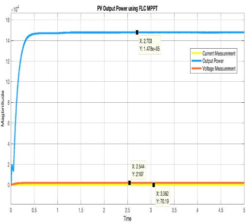
This section will highlight the performance of the Fuzzy Logic controller under two separate scenarios. In the first scenario, the panel will be subjected to a constant solar irradiance of 1000 W per square meter and will have a constant internal temperature of 25 degrees Celsius as shown in Figure 6. This allows for a simple and reliable demonstration of the algorithms’ performance in terms of accuracy and speed to get the desired power output, which is 150 kW.

999 999.5 1000 1000.5

1001 Thesis_1/Irradiance Temp : Ramp-up/down Irradiance

Ir

0 0.5 1 1.5 2 2.5 3 3.5 4 4.5 5

Time (sec)

24 24.5 25 25.5 26

Temp

Figure -6 Constant Irradiance and Temperature Signals

Figure 7 illustrates the second scenario where the panel is subjected to variable irradiance and variable temperature to document the behavior of each algorithm when experiencing conditions similar to those in real life. The irradiance will vary from 1000 W per square meter to 250 W per square meter and the temperature will vary from 25 degrees Celsius to 50 degrees Celsius. There is also a period of time where the temperature is constant and the irradiance is changing and vice versa and the reason behind that is to capture the effect of each of these variable on the output power separately. Period A represents a fixed value of irradiance and temperature at 1000 W per square meter and 25℃ respectively. In Period B the temperature remained unchanged, however, the irradiance dropped from 1000 to 250 W per square meter and remained this way from the 1.7-second mark until 2.5 seconds. Period C commenced after the 2.5 second mark, increasing the voltage back to 1000 W per square meter. Finally, in period D, the first change in the temperature is witnessed from 25 ℃ to 50 ℃ with an irradiance of 1000 W per square meter.

0 500 1000

Thesis_1/Irradiance Temp1 : Ramp-up/down Irradiance

Ir

0 0.5 1 1.5 2 2.5 3 3.5 4 4.5 5

Time (sec)

20 30 40 50

M

a

g

n

it

u

d

e Temp

A B C D

Figure -7 Varying Irradiance and Temperature Signals

3.1 SCENARIO 1: CONSTANT IRRADIANCE AND

TEMPERATURE

Figure -8 Output Power Under Constant Conditions Using FLC MPPT

The step response of the output power using fuzzy logic controller in Figure 8 results in a rise time of the output power of about 0.198 seconds and settling time of about 0.26 seconds. Moreover, the output power reaches a maximum value of about 148,100 W at time 4.675 seconds. However, the mean value of the output power is 148,000 W and when compared to the targeted output power, which is 150,000 W, results in an output efficiency of about 98.66% for the FLC.

© 2019, IRJET | Impact Factor value: 7.211 | ISO 9001:2008 Certified Journal

| Page 1404

70.2 Amperes for the output system current.

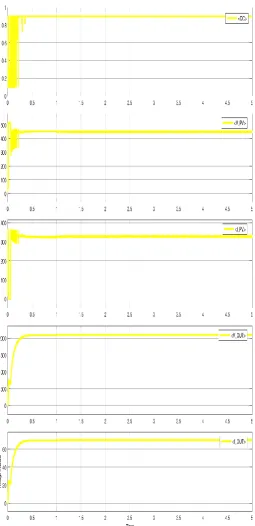
Figure -9 FLC DC, Voltage, and Current Diagrams Under Constant Conditions

3.2 SCENARIO 2: VARYING IRRADIANCE AND

TEMPERATURE

Figure -10 Output Power Under Varying Conditions Using FLC MPPT

In Figure 10, period A is where the irradiance is 1000 W per square meter and the module temperature is 25 ℃. The output power curve increases here from zero to 147,600 W of power. It then drops down to about 33,770 W in period B when the irradiance drops to 250 W per square meter and the temperature is kept constant. In part C, the irradiance increases again to 1000 W per square meter and thus the power output is close to that in part A, which is 147,200 W. Part C is done in preparation for part D, where the irradiance is kept constant at 1000 W per square meter and the temperature increases from 25 to 50 ℃. This results in a power output drop from 147,200 W to 133,900 W.

As expected, the drop in the irradiance causes the most deterioration in output power where the change from 1000 W per square meter to 250 W per square caused a 77.2% drop in the output power. On the other hand, the increase in temperature from 25 ℃ to 50 ℃ causes a percentage drop in power by about 9%.

Table 1 demonstrates the efficiency levels calculated using Equation 5.1, which are: 98.0% in period A, 92.43% in period B, 97.74% in period C, and 98.97% in period D. FLC achieved staggering efficiency percentages across all four periods.

Table -1:FLC Efficiency Percentages of each Period

Per iod

Irradia nce Value (W/m ^2)

Temperat ure Value

(℃)

Actual Output Power (W)

Theoretic al Output Power

(W)

Efficien cy Percent

age %

A 1000 25 147,600 150,600 98.00

B 250 25 33,700 36,460 92.43

C 1000 25 147,200 150,600 97.74

© 2019, IRJET | Impact Factor value: 7.211 | ISO 9001:2008 Certified Journal

| Page 1405

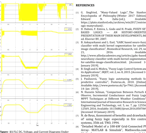
current, and the system output voltage and current. Regarding the PV’s voltage and current response, the current is highly affected by the drop in irradiance from 326 Amperes to about a mean value of 75 Amperes and no change is observed during the increase in temperature. However, the PV voltage does not seem to be affected much by either change but is affected more by the temperature where it drops from 453 Volts in period A to 451 Volts in period B and 401 Volts in period D. The two final curves are of the load side voltage and current which react in the same manner they start at with values of 2101 Volts and 70.04 Amperes respectively in period A, dropping to 1006 Volts and 33.5 Amperes in period B, increasing back up to 2101 Volts and 70.03 Amperes in period C, and finally slightly dropping to 2005 Volts and 66.8 Amperes in period D.

Figure -11 FLC DC, Voltage, and Current Diagrams Under Varying Conditions

4. CONCLUSION

This paper presented a Fuzzy Logic approach to modeling and simulating a photovoltaic system with a maximum power point controller. Fuzzy Logic was used because it is considered to be a high level controller. The PV system was designed and simulated using MATLAB/Simulink to generate a power output equivalent to 150 kW. Results of the modeling and simulation show a rise time of 0.198 seconds, settling time of 0.26 seconds, and a mean efficiency of 98.66%. The controller was subjected to four conditions of varied irradiance and temperature. Throughout Periods A to C, the temperature was kept constant at 25 degrees Celsius while the irradiance was varied. In Period D, the temperature is varied from 25 ℃ to 50 ℃. Results of the four conditions show that the maximum efficiency was reached in Period D, followed by Periods A, C, and finally B.

REFERENCES

[1] G. Siegfried, "Many-Valued Logic", The Stanford

Encyclopedia of Philosophy (Winter 2017 Edition), Edward N. Zalta (ed.), Available: https://plato.stanford.edu/archives/win2017/entries/l ogic-manyvalued/.

[2] D. Dubois, F. Esteva, L. Godo and H. Prade, FUZZY-SET

BASED LOGICS — AN HISTORY-ORIENTED PRESENTATION OF THEIR MAIN DEVELOPMENTS, 8th ed. Elsevier BV, 2007.

[3] B. Ankayarkanni and L. Ezel, "GABC based neuro-fuzzy

classifier with multi kernel segmentation for satellite image classification", Biomedical Research, vol. 29, no.

21, 2016. Available:

http://www.alliedacademies.org/articles/gabc-based- neurofuzzy-classifier-with-multi-kernel-segmentation-for-satellite-image-classification.html. [Accessed 14 January 2019].

[4] B. Singh and A. Mishra, "Fuzzy Logic Control System and

its Applications", IRJET, vol. 2, no. 8, 2015. [Accessed 14 January 2019].

[5] J. Paulusová, "Fuzzy logic autotuning methods for

predictive controller", Posterus.sk, 2010. [Online]. Available: http://www.posterus.sk/?p=7961. [Accessed: 14- Jan- 2019].

[6] N. Hussein Selman, "Comparison Between Perturb &

Observe, Incremental Conductance and Fuzzy Logic MPPT Techniques at Different Weather Conditions", International Journal of Innovative Research in Science, Engineering and Technology, vol. 5, no. 7, pp. 12556-12569, 2016. Available: 10.15680/ijirset.2016.0507069 [Accessed 10 January 2019].

[7]

N. de Reus, Assessment of benefits and drawbacks

of' using fuzzy logic especially in fire control

systems, 35th ed. TNO, 1994.

[8]

"Detailed Model of a 100-kW Grid-Connected PV

Array- MATLAB & Simulink", Mathworks.com,

© 2019, IRJET | Impact Factor value: 7.211 | ISO 9001:2008 Certified Journal

| Page 1406

https://www.mathworks.com/help/physmod/sps

/examples/detailed-model-of-a-100-kw-grid-connected-pv-array.html. [Accessed: 21- Jan-

2019].

BIOGRAPHIES

Mohamed Khallaf Born in 1996. Graduated with a BSc in Electrical Engineering and a minor in Computer Engineering from the American University of Sharjah in 2016. Currently pursuing MSc in Electrical Engineering (in Control Systems) at RIT Dubai.

Currently working as a Business Development Manager in the Energy sector in UAE for an international consulting firm. His research interests include Artificial Intelligence, Renewable Energy and Control Systems.

Abdulla Ismail Professor of Electrical Engineering. Emirati citizen, Born in Sharjah. BSc (‘80), MSc (’83), and PhD (’86) in Electrical Engineering from University of Arizona, USA. 1st Emirati to hold a PhD in Engineering. Has over 30 years of teaching and research experience at UAE University (ALAIN) and RIT Dubai.