Machine Learning in Compiler Optimization

PROCEEDINGS OF IEEE 1

Machine Learning in Compilers

Zheng Wang and Michael O’Boyle

Abstract—In the last decade, machine learning based com-pilation has moved from an an obscure research niche to a mainstream activity. In this article, we describe the rela-tionship between machine learning and compiler optimisation and introduce the main concepts of features, models, training and deployment. We then provide a comprehensive survey and provide a road map for the wide variety of different research areas. We conclude with a discussion on open issues in the area and potential research directions. This paper provides both an accessible introduction to the fast moving area of machine learning based compilation and a detailed bibliography of its main achievements.

Index Terms—Compiler, Machine Learning, Code Optimisa-tion, Program Tuning

I. INTRODUCTION

“Why would anyone want to use machine learning to build a compiler?” It’s a view expressed by many colleagues over the last decade. Compilers translate programming languages writ-ten by humans into binary executable by computer hardware. It is serious subject studied since the 50s [1], [2], [3] where correctness is critical and caution is a by-word. Machine-learning on the other hand is an area of artificial intelligence aimed at detecting and predicting patterns. It is a dynamic field looking at subject as diverse as galaxy classification [4] to predicting elections based on tweeter feeds [5]. When an open-source machine learning compiler was announced by IBM in 2009 [6], some wry slashdots commentators picked up on the AI aspect, predicting the start of sentient computers, global net and the war with machines from the Terminator film series.

In fact as we will see in this article, compilers and machine learning are a natural fit and have developed into an established research domain.

A. It’s all about optimsiation

Compiler have two jobs – translation and optimisation. They must first translate programs into binary correctly. Secondly they have to find the most efficient translation possible. There are many different correct translations whose performance varies significantly. The vast majority of research and engineering practices is focussed on this second goal of performance, traditionally misnamed optimisation. The goal was misnamed because in most cases, till recently finding an optimal translation was dismissed as being too hard to find and an unrealistic endeavour1_{. Instead it focussed on} developing compiler heuristics to transform the code in the

Z. Wang is with MetaLab, School of Computing and Communications, Lancaster University, U. K. E-mail: [email protected]

M. O’Boyle is with School of Informatics, University of Edinburgh, U. K. E-mail: [email protected]

1_{In fact the term superoptimiser [7] was coined to describe systems that}

tried to find the optimum

hope of improving performance but could in some instances damage it.

Machine learning predicts an outcome for a new data point based on prior data. In its simplest guise it can be considered a from of interpolation. This ability to predict based on prior information can be used to find the data point with the best outcome and is closely tied to the area of optimisation. It is at this overlap of looking at code improvement as an optimisation problem and machine learning as a predictor of the optima where we find machine-learning compilation.

Optimisation as an area, machine-learning based or other-wise, has been studied since the 1800s [8], [9]. An interesting question is therefore why has has the convergence of these two areas taken so long? There are two fundamental reasons. Firstly, despite the year-on year increasing potential perfor-mance of hardware, software is increasingly unable to realise it leading to a software-gap. This gap has yawned right open with the advent of multi-cores (see also Section VI-B). Compiler writers are looking for new ways to bridge this gap.

Secondly, computer architecture evolves so quickly, that it is difficult to keep up. Each generation has new quirks and compiler writers are always trying to play catch-up. Machine learning has the desirable property of being automatic. Rather than relying on expert compiler writers to develop clever heuristics to optimise the code, we can let the machine learn how to optimise a compiler to make the machine run faster, an approach sometimes referred to as auto-tuning [10], [11].

Machine learning is part of a tradition in computer science and compilation in increasing automation The 50s to 70s were spent trying to automate compiler translation, e.g. lex for lexical analysis [12] and yacc for parsing [13], the last decade by contrast has focussed on trying to automating compiler optimisation. As we will see it is not “magic” or a panacea for compiler writers, rather it is another tool allowing automation of tedious aspects of compilation providing new opportunities for innovation. It also brings compilation nearer to the stan-dards of evidence based science. It introduces an experimental methodology where we separate out evaluation from design and considers the robustness of solutions. Machine learning based schemes in general have the problem of relying on black-boxes whose working we do not understand and hence trust. This problem is just as true for machine learning based compilers. In this paper we aim to demystify machine learning based compilation and show it is a trustworthy and exciting direction for compiler research.

for(…) { ... }

#inst. #load #branch cache miss rate

Training programs

...

... Fe

at

ure

s o

f

tr

aining

pr

og

ram

s

Optimal options +

Supervised Machine

Learner

Model

New program

Features for new program

Prediction Model

(a) Feature engineering (b) Learning a model (c) Deployment

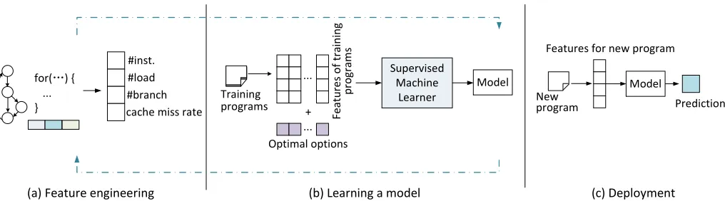
Fig. 1: A generic view of supervised machine learning in compilers. In the feature engineering stage (a), the compiler developer investigates data structures that are important to the problem. The data structures will typically be summarised as feature vectors. In the learning stage (b), representative training programs are used to generate training examples. Each example consists of feature vectors and the optimal compiler decision for each program. These training examples are fed into a machine learning algorithm to automatically learn a model. In the deployment stage (c), the learned model is inserted into the compiler to predict the best compiler decisions for new programs.

models that have been employed in prior work. Next, in Section V, we review how previous work chooses quantifiable properties, or features, to represent programs. We discuss the challenges and limitations for applying machine learning to compilation, as well as open research directions in Section VII before we summarise and conclude in Section VIII.

II. OVERVIEW OFMACHINELEARNING INCOMPILERS

Given a program, compiler writers would like to know what compiler heuristic or optimisation to apply in order to make the code better. Better often means execute faster, but can also mean smaller code footprint or reduced power. Machine learning can be used to build a model used within the compiler, that makes such decisions for any given program.

There are two main stages involved: learning and deploy-ment. The first stage learns the model based on training data, while the second uses the model on new unseen programs. Within the learning stage, we needs a way of representing programs in a systematic way. This representation is known as the program features [14].

Figure 1 gives a intuitive view how machine learning can be applied to compilers. This process which includes feature engineering, learning a model and deployment is described in the following sub-sections.

A. Feature engineering

Before we can learn anything useful about programs, we first need to be able to characterise them. Machine learn-ing relies on a set of quantifiable properties, or features, to characterise the programs (Figure 1a). There are many different features that can be used. These include the static data structures extracted from the program source code or the compiler intermediate representation (such as the number of instructions or branches), dynamic profiling information (such as performance counter values) obtained through runtime profiling, or a combination of the both.

Standard machine learning algorithms typically work on fixed length inputs, so the selected prosperities will be sum-marised into a fixed length feature vector. Each element of

the vector can be an integer, real or Boolean value. The process of feature selection and tuning is referred as feature engineering. This process may need to iteratively perform multiple times to find a set of high-quality features to build a accurate machine learning model. In Section V, we provide a comprehensive review of feature engineering for the topic of program optimisation.

B. Learning a model

The second step is to use training data to derive a model us-ing a learnus-ing algorithm. This process is depicted in Figure 1b. Unlike other applications of machine learning, we typically generate our own training data. The compiler developer will select training programs which are typical of the application domain. For each training program, we calculate the feature values, compiling the program with different optimisation options, and running and timing the compiled binaries to discover the best-performing option. This process produces, for each training program, a training instance that consists of the feature values and the optimal compiler option for the program.

The compiler developer then feeds these examples to a machine learning algorithm to automatically build a model. The learning algorithms job is to find from the training examples a correlation between the feature values and the optimal optimisation decision. The learned model can then be used to predict, for a new set of features, what the optimal optimisation option should be.

Because the performance of the learned model strongly depends on how well the features and training programs are chosen, so that the processes of featuring engineering and training data generation often need to repeat multiple times.

C. Deployment

PROCEEDINGS OF IEEE 3

1 k e r n e l v o i d s q u a r e ( g l o b a l f l o a t∗ i n , g l o b a l f l o a t∗ o u t ){

2 i n t g i d = g e t g l o b a l i d ( 0 ) ; 3 o u t [ g i d ] = i n [ g i d ] ∗ i n [ g i d ] ; 4 }

(a) Original OpenCL kernel

1 k e r n e l v o i d s q u a r e ( g l o b a l f l o a t∗ i n , g l o b a l f l o a t∗ o u t ){

2 i n t g i d = g e t g l o b a l i d ( 0 ) ; 3 i n t t i d 0 = 2∗g i d + 0 ; 4 i n t t i d 1 = 2∗g i d + 1 ;

5 o u t [ t i d 0 ] = i n [ t i d 0 ] ∗ i n [ t i d 0 ] ; 6 o u t [ t i d 1 ] = i n [ t i d 1 ] ∗ i n [ t i d 1 ] ; 7 }

(b) Code transformation with a coarsening factor of 2

Fig. 2: An OpenCL thread coarsening example reproduced from [15]. The original OpenCL code is shown at (a) where each thread takes the square of one element of the input array. When coarsened by a factor of two (b), each thread now processes two elements of the input array.

program, and then feeds the extracted feature values to the learned model to make a prediction.

The advantage of the machine learning based approach is that the entire process of building the model can be easily repeated whenever the compiler needs to target a new hardware architecture, operating system or application domain. The model built is entirely derived from experimental results and is hence evidence based.

D. Example

As an example to illustrate these steps, consider thread coarsening [16] for GPU programs. This code transformation technique works by giving multiple work-items (or work elements) to one single thread. It is similar to loop unrolling, but applied across parallel work-items rather than across serial loop iterations.

Figure 2 (a) shows a simple OpenCL kernel where a thread operates on a work-item of the one-dimensional input array,

in, at a time. The work-item to be operated on is specified by the value returned from the OpenCLget_global_id()

API. Figure 2 (b) shows the transformed code after applying a thread coarsen factor of two, where each thread processes two elements of the input array.

Thread coarsening can improve performance through in-creasing instruction-level parallelism [17], reducing the num-ber of memory-access operations [18], and eliminating redun-dant computation when the same value is computed in every work-item. However, it can also have several negative side-effects such as reducing the total amount of parallelism and increasing the register pressure, which can lead to slowdown performance. Determining when and how to apply thread coarsening is non-trivial, because the best coarsening factor depends on the target program and the hardware architecture that the program runs on [17], [15].

Magni et al. show that machine learning techniques can be used to automatically construct effective thread-coarsening

TABLE I: Candidate code features used in [15].

Feature Desc. Feature Desc.

# Basic Blocks # Branches

# Divergent Instr. # Instrs. in Divergent Regions (# instr. in Divergent regions)/(# total

instr.)

# Divergent regions # Instrs # Floating point instr.

Avg. ILP per basic block (# integer instr.) / (# floating point instr.) # integer instr. # Math built-in func.

Avg. MLP per basic block # loads

# stores # loads that are independent of the coarsening direction

# barriers

heuristics across GPU architectures [15]. Their approach con-siders six coarsening factors, (1,2,4,8,16,32). The goal is to develop a machine learning based model to decide whether an OpenCL kernel should be coarsened on a specific GPU architecture and if so what is the best coarsening factor. Among many machine learning algorithms, they chose to use an artificial neural network to model2the problem. Construing such a model follows the classical 3-step supervised learning process, described as follows.

a) Feature engineering: To describe the input OpenCL kernel, Magni et al. use static code features extracted from the compiler’s intermediate representation. Specifically, they developed a compiler-based tool to obtain the feature values from the program’s LLVM bitcode [19]. They started from 17 candidate features. These include things like the number of and types of instructions and memory level parallelism (MLP) within an OpenCL kernel. Table I gives the list of candidate features used in [15]. Typically, candidate features can be chosen based on developers’ intuitions, suggestions from prior works, or a combination of both. After choosing the candidate features, a statistical method called Principal Component Analysis (see also Section IV-B) is applied to map the 17 candidate features into 7 aggregated features, so that each aggregated feature is a linear combination of the original features. This technique is known as “feature dimension reduction” which is discussed at Section V-D2. Dimension reduction helps eliminating redundant information among candidate features, allowing the learning algorithm to perform more effectively.

b) Learning the model: For the work presented in [15], 16 OpenCL benchmarks were used to generate training data. To find out which of the six coarsening factors performs best for a given OpenCL kernel on a specific GPU architecture, we can apply each of the six factors to an OpenCL kernel and records its execution time. Since the optimal thread-coarsening factor varies across hardware architectures, this process needs to repeat for each target architecture. In addition to finding the best-performing coarsening factor, Magniet al.also extracted the aggregated feature values for each kernel. Applying these two steps on the training benchmarks results in a training dataset where each training example is composed of the opti-mal coarsening factor and feature values for a training kernel. The training examples are then fed into a learning algorithm

2_{In fact, Magniet al.employed a hieratical approach consisting of multiple}

Compiler heuristic

available options

Cost function Continue?

evaluate an option quality metric

input program

best-found option No

Yes

input program

Feature extraction

features

Predictive

model predicted option (a) Use a cost function to guide compiler decisions

Compiler heuristic

available options

Cost function Continue?

evaluate an option quality metric

input program

best-found option No

Yes

input program

Feature extraction

features

Predictive

model predicted option

(b) Use a model to directly predict the decision

Fig. 3: There are in general two approaches to determine the optimal compiler decision using machine learning. The first one is to learn a cost or priority function to be used as a proxy to select the best-performing option (a). The second one is to learn a predictive model to directly predict the best option.

which tries to find a set of model parameters (or weights) so that overall prediction error on the training examples can be minimised. The output of the learning algorithm is an artificial neural network model where its weights are determined from the training data.

c) Deployment: The learned model can then be used to predict the optimal coarsening factor for unseen OpenCL programs. To do so, static source code features are first extracted from the target OpenCL kernel; the extracted feature values are then fed into the model which decides whether to coarsen or not and which coarsening factor should use. The technique proposed in [15] achieves an average speedup between 1.11x and 1.33x across four GPU architectures and does not lead to degraded performance on a single benchmark.

III. METHODOLOGY

One of the key challenges for compilation is to select the right code transformation, or sequence of transformations for a given program. This requires effectively evaluating the quality of a possible compilation option e.g. how will a code transformation affect eventual performance.

A naive approach is to exhaustively apply each legal transformation option and then profile the program to collect the relevant performance metric. Given that many compiler problems have a massive number of options, exhaustive search and profiling is infeasible, prohibiting the use of this approach at scale. This search based approach to compiler optimisation is known as iterative compilation [20], [21] or auto-tuning [10], [22]. Many techniques have been proposed to reduce the cost of searching a large space [23], [24]. In certain cases, the overhead is justifiable if the program in question is to be used many times e.g. in a deeply embedded device. However, its main limitation remains: it only finds a good optimisation for one program and does not generalise into a compiler heuristic. There are two main approaches for solving the problem of scalably selecting compiler options that work across programs. A high level comparison of both approaches is given in Figure 3. The first strategy attempts to develop a cost (or priority) function to be used as a proxy to estimate the quality

of a potential compiler decision, without relying on extensive profiling. The second strategy is to directly predict the best-performing option.

A. Building a cost function

Many compiler heuristics rely on a cost function to es-timate the quality of a compiler option. Depending on the optimisation goal, the quality metric can be execution time, the code size, or energy consumption etc. Using a cost function, a compiler can evaluate a range of possible options to choose the best one, without needing to compile and profile the program with each option.

1) The problem of hand-crafted heuristics: Traditionally, a compiler cost function is manually crafted. For example, a heuristic of function inlining adds up a number of relevant metrics, such as the number of instructions of the target function to be inlined, the callee and stack size after inlining, and compare the resulted value against a pre-defined threshold to determine if it is profitable to inline a function [25]. Here, the importance or weights for metrics and the threshold are determined by compiler developers based on their experience or via “trail-and-error”. Because the efforts involved in tuning the cost function is so expensive, many compilers simply use “one-size-fits-all” cost function for inlining. However, such a strategy is ineffective. For examples, Cooper et al.show that a “one-size-fits-all” strategy for inlining often delivers poor performance [26]; other studies also show that that the optimal thresholds to use to determine when to inline changes from one program to the other [27], [28].

Hand-crafted cost functions are widely used in compilers. Other examples include the work conducted by Wagner et al.[29] and Tiwariet al.[30]. The former combines a Markov model and a human-derived heuristic to statically estimate the execution frequency of code regions (such as function innova-tion counts). The later calculates the energy consumpinnova-tion of an applicaiton by assigning a weight to each instruction type. The efficiency of these approaches highly depend on the accuracy of the estimations given by the manually tuned heuristic.

The problem of relying on a hand-tuned heuristic is that the cost and benefit of a compiler optimisation often depends on the underlying hardware; while hand-crafted cost functions could be effective, manually developing one can take months or years on a single architecture. This means that tuning the compiler for each new released processor is hard and is often infeasible due to the drastic efforts involved. Because cost functions are important and manually tuning a good function is difficult for each individual architecture, researchers have investigated ways to use machine learning to automate this process.

In the next subsection, we review a range of previous studies on using machine learning to tune cost functions for performance and energy consumption – many of which can be applied to other optimisation targets such as the code size [31] or a trade-off between energy and runtime.

PROCEEDINGS OF IEEE 5

+

#inst.

/

4.0

x

#branches

#loads

Generate inital

cost functions

Evaluate

functions

Keep

well-performing

functions

Randomize the

expressions to create

new functions

(a) An example cost function in [32] +

#inst. /

4.0 x

#branches #loads

Generate inital cost functions

Evaluate functions

Keep well-performing

functions

Create new functions using remaining ones

Continue? Yes

No Exit

(b) A simple view of the generic programming technique in [32]

Fig. 4: A simple view of the genetic programming (GP) approach presented at [32] for tuning compiler cost functions. Each candidate cost function is represented as an expression tree (a). The workflow of theGPalgorithm is presented at (b).

x, and produces a real-valued priority, y. Figure 4 depicts the workflow of the framework. This approach is evaluated on a number of compiler problems, including hyperblock formation3_{, register allocation, and data prefetching, showing} that machine learned cost functions outperform human-crafted ones. A similar approach is employed by Cavazos et al.find cost functions for performance and compilation overhead for a Java just-in-time compiler [33]. The COLE compiler [34] uses a variance of the GP algorithm called Strength Pareto Evolutionary Algorithm2 (SPEA2) [35] to learn cost functions to balance multiple objectives (such as program runtime, compilation overhead and code size). In Section IV-C, we describe the working mechanism ofGP-like search algorithms. Another approach to tune the cost functions is to predict the execution time or speedup of the target program. The Qilin compiler [36] follows such an approach. It uses curve fitting algorithms to estimate the runtime for executing the target program of a given input size on the CPU and the GPU. The compiler then uses this information to determine the optimal loop iteration partition across the CPU and the GPU. The Qilin compiler relies on an application-specific function which is built on a per program base using reference inputs. The curve fitting (or regression – see also Section IV) model employed by the Qilin compiler can model with continuous values, making it suitable for estimating runtime and speedup. In [37], this approach is extended, which developed a relative predictor that predicts whether an unseen predictor will improve significantly on a GPU relative to a CPU. This is used for runtime scheduling of OpenCL jobs.

The early work conduced by Brewer proposed a regression-based model to predict the execution of a data layout scheme for parallelization, by considering three parameters [38]. Using the model, their approach can select the optimal layout for over 99% of the time for a Partial Differential Equations (PDE) solver across four evaluation platforms. Other previous works also use curve fitting algorithms to build a cost function to estimate the speedup or runtime of sequential [39], [40], [41], OpenMP [42], [43], [44], and more recently for deep learning applications [45].

3) Cost functions for energy consumption: In addition to performance, there is an extensive body of work investigates ways to build energy models for software optimisation and

3_{Hyperblock formation combines basic blocks from multiple control paths}

to form a predicated, larger code block to expose instruction level parallelism.

hardware architecture design. As power or energy readings are continuous real values, most of the prior work on power modelling use regression-based approaches.

Linear regression is a widely used technique for energy modeling. Benini et al. developed a linear regression-based model to estimate power consumption at the instruction lev-el [46]. The framework presented by Rethinagiri et al.. [47] uses parameterised formulas to estimate power consumption of embedded systems. The parameters of the formulas are determined by applying a regression-based algorithm to refer-ence data obtained with hand-crafted assembly code and power measurements. In a more recent work, Sch¨urmanset al.also adopt a regression-based method for power modelling [48], but the weights of the regression model are determined using standard benchmarks instead of hand-written assembly pro-grams.

Other works employ the artificial neural network (ANN) to automatically construct power models. Curtis-Mauryet al. develop an ANN-based model to predict the power consump-tion of OpenMP programs on multi-core systems [49]. The inputs to the model are hardware performance counter values such as the cache miss rate, and the output is the estimated power consumption. Su et al. adopt a similar approach by developing an ANN predictor to estimate the runtime and power consumption for mapping OpenMP programs on Non-Uniform Memory Access (NUMA) multi-cores. This approach is also based on runtime profiling of the target program, but it explicitly considers NUMA-specific information like local and remote memory accesses per cycle.

B. Directly predict the best option

While a cost function is useful for evaluating the quality of compiler options, the overhead involved in searching for the optimal option may still be prohibitive. For this reason, researchers have investigated ways to directly predict the best compiler decision using machine learning for relatively small compilation problems.

Later, Stephenson and Amarasinghe advanced [14] by directly predicting the loop unroll factor [50] by considering eight unroll factors, (1,2, . . . ,8). They formulated the problem as a multi-class classification problem (i.e. each loop unroll factor is a class). They used over 2,500 loops from 72 benchmarks to train two machine learning models (a nearest neighbor and a support vector machines model) to predict the loop unroll factor for unseen loops. Using a richer set of features than [14], their techniques correctly predict the unroll factor for 65% of the testing loops, leading to on average, a 5% improvement for the SPEC 2000 benchmark suite.

For sequential programs, there is extensive work in pre-dicting the best compiler flags [51], [52], code transformation options [53], or tile size for loops [54], [55]. This level of interest is possibly due to the restricted nature of the problem, allowing easy experimentation and comparision against prior work.

Directly predicting the optimal option for parallel programs is harder than doing it for sequential programs, due to the complex interactions between the parallel programs and the underlying parallel architectures. Nonetheless, there are works on predicting the optimal number of threads to use to run an OpenMP program [44], [56], the best parameters to used to compile a CUDA programs for a given input [57] the thread coarsening parameters for OpenCL programs for GPUs [15]. These papers show that supervised machine learning can be a powerful tool for modelling problems with a relatively small number of optimisation options.

IV. MACHINELEARNINGMODELS

In this section, we review the wide range of machine learning models used for compiler optimisation.

There are two major subdivisions of machine learning techniques that have previously been used in compiler opti-misations: supervised and unsupervised learning. Using su-pervised machine learning, a predictive model is trained on empirical performance data (labelled outputs) and important quantifiable properties (features) of representative programs. The model learns the correlation between these feature values and the optimisation decision that delivers the optimal (or nearly optimal) performance. The learned correlations are used to predict the best optimisation decisions for new programs. Depending on the nature of the outputs, the predictive model can be either a regression model for continuous outputs or a classification model for discrete outputs.

In the other subdivision of machine learning, termed unsu-pervised learning, the input to the learning algorithm is a set of input values merely – there is no labelled output. One form of unsupervised learning is clusteringwhich groups the input data items into several subsets. For example, SimPoint [58], a simulation technique, uses clustering to pick represent program execution points for program simulation. It does so by first dividing a set of program runtime information into groups (or clusters), such that points within each cluster are similar to each other in terms of program structures (loops, memory usages etc.); it then chooses a few points of each cluster to represent all the simulation points within that group without losing much information.

X

Y

_f(x)

_y

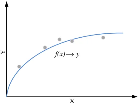
Fig. 5: A simple regression-based curve-fitting example. There are five training examples in this case. A function,f, is trained with the training data, which maps the input xto the output

y. The trained function can predict the output of an unseenx.

There are also techniques that sit at the boundary of supervised and unsupervised learning. These techniques refine the knowledge gathered during offline learning or previous runs using empirical observations obtained during deployment. We review such techniques in Section IV-C. This sections concludes with a discussion of the relative merits of different modelling approaches for compiler optimisation.

A. Supervised learning

1) Regression: A widely used supervised learning tech-nique is called regression. This technique has been used in various tasks, such as predicting the program execution time input [36] or speedup [37] for a given input, or estimating the tail latency for parallel workloads [59].

Regression is essentially curve-fitting. As an example, con-sider Figure 5 where a regression model is learned from five data points. The model takes in a program input size, X, and predicts the execution time of the program,Y. Adhering to supervised learning nomenclature, the set of five known data points is the training data set and each of the five points that comprise the training data is called a training example. Each training example,(xi, yi), is defined by a feature vector (i.e. the input size in our case),xi, and a desired output (i.e. the program execution time in our case),yi. Learning in this context is understood as discovering the relation between the inputs (xi) and the outputs (yi) so that the predictive model can be used to make predictions for any new, unseen input features in the problem domain. Once the function, f, is in place, one can use it to make a prediction by taking in a new input feature vector,x. The prediction,y, is the value of the curve that the new input feature vector,x, corresponds to.

PROCEEDINGS OF IEEE 7 TABLE II: Regression techniques used in prior works.

Modelling Technique Application References

Linear Regression Exec. Time Estimation [60], [36], [41]

Linear Regression Perf. & Power Prediction [61], [62], [63] Artificial Neural Networks Exec. Time Estimation [60], [44], [37]

F1 (Commun. - Computation Ratio) < 0.03

F4 (Computation – Mem Ratio) < 7.65

F3 < 21

F2 ( % Coalesced Mem Access) < 0.99

F3 (% Local Mem Access Avg. #Work-items per Kernel) < 3300

CPU GPU

CPU GPU

F3 < 0.02

GPU

F4 < 134

GPU

F4 < 30

GPU CPU

No Yes

GPU

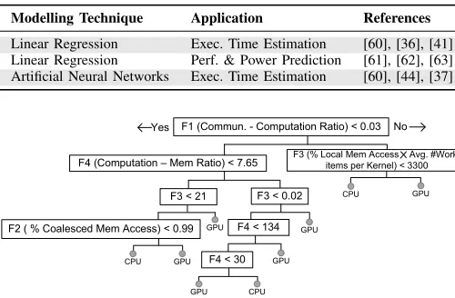
Fig. 6: A decision tree for determining which device (CPU or GPU) to use to run an OpenCL program. This diagram is reproduced from [66].

output (i.e. labels) have a strong linear relation.SVMandANNs

can model both linear and non-linear relations, but typically require more training examples to learn an effective model when compared with simple linear regression models.

Table II gives some examples of regression techniques that have been used in prior work for code optimisation and the problem to be modelled.

2) Classification: Supervised classification is another tech-nique that has been widely used in prior work of machine learning based code optimisation. This technique takes in a feature vector and predicts which of a set of classes the feature vector is associated with. For example, classification can be used to predict which of a set of unroll factors should be used for a given loop, by taking in a feature vector that describes the characteristics of the target loop (see also Section II-D).

The k-nearest neighbour (KNN) algorithm is a simple yet effective classification technique. It finds the kcloset training examples to the input instance (or program) on the feature space. The closeness (or distance) is often evaluated using the Euclidean distance, but other metrics can also be used. This technique has been used to predict the optimal optimisation parameters in prior works [50], [64], [65]. It works by first predicting which of the training programs are closet (i.e. near-est neighbours) to the incoming program on the feature space; it then uses the optimal parameters (which are found during training time) of the nearest neighbours as the prediction output. While it is effective on small problems, KNNalso has two main drawbacks. Firstly, it must compute the distance between the input and all training data at each prediction. This can be slow if there is a large number of training programs to be considered. Secondly, the algorithm itself does not learn from the training data; instead, it simply selects thek nearest neighbours. This means that the algorithm is not robust to noisy training data and could choose an ill-suited training program as the prediction.

As an alternative, the decision tree has been used in prior works for a range of optimisation problems. These include choosing the parallel strategy for loop parallelisation [67],

Compiler heuristic

available options

Cost function Continue?

evaluate an option quality metric

input program

best-found option

No

Yes

input program

Feature extraction

feature vector x

Predictive

model predicted option

Tree 1 Tree 2

Tree n

...

y1

y2

yn

Prediction

yout= ∑ wiyi

Random Forests

Fig. 7: Random forests are an ensemble learning algorithm. It aggregates the outputs of multiple decision trees to form a final prediction. The idea is to combine the predictions from multiple individual models together to make a more robust, accurate prediction than any individual model.

determining the loop unroll factor [14], [68], deciding the prof-itability of using GPU acceleration [66], [69], and selecting the optimal algorithm implementation [70]. The advantage of a decision tree is that the learned model is interpretable and can be easily visualised. This enables users to understand why a particular decision is made by following the path from the root node to a leaf decision node. For example, Figure 6 depicts the decision tree model developed in [66] for selecting the best-performing device (CPU or GPU) to run an OpenCL program. To make a prediction, we start from the root of the tree; we compare a feature value (e.g. the communication-computation ratio) of the target program against a threshold to determine which branch of the tree to follow; and we repeat this process until we reach a leaf node where a decision will be made. It is to note that the structure and thresholds of the tree are automatically determined by the machine learning algorithm, which may change when we target a different architecture or application domain.

Decision trees make the assumption that the feature space is convex i.e. it can be divided up using hyperplanes into different regions each of which belongs to a different category. This restriction is often appropriate in practice. However, a significant drawback of using a single decision tree is that the model can over-fit due to outliers in the training data (see also Section IV-D). Random forests [71] have therefore been proposed to alleviate the problem of over fitting. Random forests are an ensemble learning method [72]. As illustrated in Figure 7, it works by constructing multiple decision trees at training time. The prediction of each tree depends on the values of a random vector sampled independently on the feature value. In this way, each tree is randomly forced to be insensitive to some feature dimensions. To make a prediction, random forests then aggregate the outcomes of individual trees to form an overall prediction. It has been employed to determine whether to inline a function or not [73], delivering better performance than a single-model-based approach. We want to highlight that random forests can also be used for re-gression tasks. For instances, it has been used to model energy consumption of OpenMP [74] and CUDA [75] programs.

CF: 2 CF: 2 CF: 4 CF: 1

Source Code

DNN 2

Output Layer DNN 1

AMD HD 5900 AMD Tahiti 7970 NVIDIA GTX 480 NVIDIA Tesla K20c AMD HD 5900

AMD Tahiti 7970 NVIDIA GTX 480 NVIDIA Tesla K20c

AMD HD 5900 AMD Tahiti 7970 NVIDIA GTX 480 NVIDIA Tesla K20c

Outputs of DNN 1

Output of DNN 2

Processing Layer

kernel void square ( global float* in , global float* out ){

int gid = get_global_id (0) ;

out [ gid ] = in [ gid ] * in [ gid ];

... }

(a)

(b)

(c)

(d)

Fig. 8: A simplified view of the internal state for the DeepTune DNN framework [76] when it predicts the optimal OpenCL thread coarsening factor. Here a DNN is learned for each of the four target GPU architectures. The activations in each layer of the four models increasingly diverge (or specialise) towards the lower layers of the model. It is to note that some of the DeepTune layers are omitted to aid presentation.

the optimisation level of Jike RVM. Like decision trees, logical regression also assumes that the feature values and the prediction has a linear relation.

More advanced models such asSVMclassification has been used for various compiler optimisation tasks [44], [77], [78].

SVMsuse kernel functions to compute the similarity of feature vectors. The radial basis function (RBF) is commonly used in prior works [44], [79] because it can model both linear and non-linear problems. It works by mapping the input feature vector to a higher dimensional space where it may be easier to find a linear hyper-plane to well separate the labelled data (or classes).

Other machine learning techniques such as Kernel Canoni-cal Correlation Analysis and naive Bayes have also been used in prior works to predict stencil program configurations [80] or detect parallel patterns [81].

3) Deep neural networks: In recent years, deep neural net-works [82] have been shown to be a powerful tool for tackling a range of machine learning tasks like image recognition [83], [84] and audio processing [85]. DNNs have recently used to model program source code [86] for various software engineer-ing tasks (see also Section VI-C), but so far there is little work of applyingDNNsto compiler optimisation. A recent attempt in this direction is the DeepTune framework [76], which uses

DNNs to extract source code features (see also Section V-C). The advantage of DNNs is that it can compactly represent a significantly larger set of functions than a shallow network, where each function is specialised at processing part of the input. This capability allowsDNNsto model the complex

rela-tionship between the input and the output (i.e. the prediction). As an example, consider Figure 8 that visualizes the internal state of DeepTune [76] when predicting the optimal thread coarsening factor for an OpenCL kernel (see Section II-D). Figure 8 (a) shows the first 80 elements of the input source code tokens as a heatmap in which each cell’s color reflects an integer value assigned to a specific token. Figure 8 (b) shows the neurons of the firstDNNfor each of the four GPU platforms, using a red-blue heatmap to visualize the intensity of each activation. If we have a close look at the heatmap, we can find that a number of neurons in the layer with different responses across platforms. This indicates that the

DNNis partly specialised to the target platform. As information flows through the network (layers c and d in Figure 8), the layers become progressively more specialised to the specific platform.

PROCEEDINGS OF IEEE 9

we can find ways to reduce the cost of generating program training data, we can then greatly extend the reach of DNNs

to compiler-based code optimisation.

B. Unsupervised learning

Unlike supervised learning models which learn a correlation from the input feature values to the corresponding outputs, unsupervised learning models only take it the input data (e.g. the feature values). This technique is often used to model the underlying structure of distribution of the data.

Clustering is a classical unsupervised learning problem. The k-means clustering algorithm [88] groups the input data into

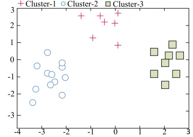
k clusters. For example, in Figure 9, a k-means algorithm is used to group data points into three clusters on a 2-dimensional feature space. The algorithm works by grouping data points that are close to each other on the feature space into a cluster. K-means is used to characterise program behaviour [58], [89]. It does so by clustering program execution into phase groups, so that we can use a few samples of a group to represent the entire program phases within a group. K-means is also used in the work presented in [90] to summarise the code structures of parallel programs that benefit from similar optimisation strategies. In addition to k-means, Martins et al. employed the Fast Newman clustering algorithm [91] which works on network structures to group functions that may benefit from similar compiler optimisations [92].

Principal Component Analysis (PCA) is a statistical method for unsupervised learning. This method has been heavily used in prior work to reduce the feature dimension [93], [23], [94], [95], [15]. Doing so allows us to model a high-dimensional feature space with a smaller number of representative variables which, in combination, describe most of the variability found in the original feature space. PCA is often used to discover the common pattern in the datasets in order to help clustering exercises. It is used to select representative programs from a benchmark suite [93], [96]. In Section V-D, we discuss PCA

in further details.

Autoencoders are a recently proposed artificial neural net-work architecture for discovering the efficient codings of input data in an unsupervised fashion [97]. This technique can be used in combination of a natural language model to first extract features from program source code and then find a compact representation of the source code features [98]. We discuss autoencoders in Section V-D when reviewing feature dimensionality reduction techniques.

C. Online learning

1) Evolutionary search: Evolutionary algorithms (EAs) or evolutionary computation like genetic algorithms, genetic pro-gramming4 and stochastic based search have been employed to find a good optimisation solution from a large search space. An EA applies a principles inspired by biological evolution to find an optimal or nearly optimal solution for

4_{A genetic algorithm (GA) is represented as a list of actions and values,}

often a string, while a genetic program (GP) is represented as a tree structure of actions and values. For example,GPis applied to the abstract syntax tree of a program to search for useful features in [68].

3

-4 -3 -2 -1 0 1 2

3

2

1

0

-1

-2

-3

Cluster-1 Cluster-2 Cluster-3

Fig. 9: Using k-means to group data points into three clusters. In this example, we group the data points into three clusters on a 2-d feature space.

the target problem. For instance, the SPIRAL auto-tuning framework uses a stochastic evolutionary search algorithm to choose a fast formula (or transformation) for signal processing applications [99]. Liet al.use genetic algorithms to search for the optimal configuration to determine which sorting algorithm to use based on the unsorted data size [100]. The Petabricks compiler offers a more general solution by using evolutionary algorithms to search for the best-performing configurations for a set of algorithms specified by the programmer [101]. In addition to code optimisation, EAs have also been used to create Pareto optimal program benchmarks under various criteria [102].

As an example, consider how an EA can be employed in the context of iterative compilation to find the best compiler flags for a program [23], [34], [103]. Figure 10 depicts how an EA can be used for this purpose. The algorithm starts from several populations of randomly chosen compiler flag settings. It compiles the program using each individual compiler flag sequence, and uses afitness functionto evaluate how well a compiler flag sequence performs. In our case, a fitness function can simply return the reciprocal of a program runtime measurment, so that compiler settings that give faster execution time will have a higher fitness score. In the next epoch, the EA algorithm generates the next populations of compiler settings via mechanisms like reproduction (cross-over) and mutation among compiler flag settings. This results in a new generation of compiler flag settings and the quality of each setting will be evaluated again. In a mechanism analogous to natural selection, a certain number of poorly performing compiler flags within a population are chosen to die in each generation. This process terminates when no further improvement is observed or the maximum number of generations is reached, and the algorithm will return the best-found program binary as a result.

... ...

...

Individual compiler flag setting compiler setting population

1st_gen.

... ...

...

2nd_gen.

... ... ...

Selection

Cross-over mutation

...

... ...

...

(N-1)th_gen.

... ... ...

... ...

...

Nth_gen.

Best-performing Binary

Fig. 10: Use an evolutionary algorithm to perform iterative compilation. The algorithm starts from several initial popula-tions of randomly chosen compiler flag sequences. It evaluates the performance of individual sequences to remove poorly performing sequences in each population. It then applies cross-over and mutation to create a new generation of populations. The algorithm returns the best-performing program binary when it terminates.

compiler flags). The likelihood of an existing option being chosen for cross-over is again proportional to its fitness. This strategy ensures that good optimisations will be preserved over generations, while poorly performing optimisations will grad-ually die out. Finally, mutation randomly changes a preserved optimisation, e.g. by turning on/off an option or replacing a threshold value in a compiler flag sequence. Mutation reduces the chance that the algorithm gets stuck with a locally optimal optimisation.

EAs are useful for exploring a large optimisation space where it is infeasible to just enumerate all possible solutions. This is because anEAcan often converge to the most promis-ing area in the optimisation space quicker than a general search heuristic. The EA is also shown to be faster than a dynamic programming based search [22] in finding the optimal transformation for the Fast Fourier Transformation (FFT) [99]. When compared to supervised learning,EAshave the advantage of requiring little problem specific knowledge, and hence that they can be applied on a broad range of problems. However, because an EA typically relies on the empirical evidences (e.g. running time) for fitness evaluation, the search time can still be prohibitively expensive. This overhead can be reduced by using a machine learning based cost model [41] to estimate the potential gain (e.g. speedup) of a configuration (see also Section III-A). Another approach is to

Environment

Learning

Algorithm

reward r(t)

state s(t)

actio

n a(

t+1)

Fig. 11: The working mechanism of reinforcement learning

combine supervised learning and evolutionary algorithms [23], [104] – by first using an offline learned model to predict the most promising areas of the design space (i.e. to narrow down the search areas), and then searching over the predicted areas to refine the solutions. Moreover, instead of predicting where in the search space to focus on, one can also first prune the search space to reduce the number of options to search over. For example, Jantz and Kulkarni show that the search space of phase ordering5 can be greatly reduced if we can first remove phases whose application order is irrelevant to the produced code [105]. Their techniques are claimed to prune the exhaustive phase order search space size by 89% on average.

2) Reinforcement learning: Another class of online learn-ing algorithms is reinforcement learnlearn-ing (RL) which is some-times called “learning from interactions”. The algorithm tries to learn how to maximise the rewards (or performance) itself. In other words, the algorithm needs to learn, for a given input, what is the correct output or decision to take. This is different from supervised learning where the correct input/output pairs are presented in the training data.

Figure 11 illustrates the working mechanism of RL. Here the learning algorithm interacts with its environment over a discrete set of time steps. At each step, the algorithm evaluate the current state of its environment, and executes an action. The action leads to a change in the state of the environment (which the algorithm can evaluate in the next time step), and produces an immediate reward. For examples, in a multi-tasking environment, a state could be the CPU contention and which processor cores are idle, an action could be where to place a process, and a reward could be the overall system throughput. The goal of RL is to maximize the long-term cumulative reward by learning an optimal strategy to map states to actions.

RLis particularly suitable for modelling problems that have an evolving natural, such as dynamic task scheduling, where the optimal outcome is achieved through a series of actions.

RLhas been used in prior resarch to schedule RAM memory traffics [106], selecting software component configurations at runtime [107], and configure virtual machines [108]. An early work of usingRLfor program optimisation was conduced by Lagoudakis and Littman [109]. They useRLto find the cut-off point to switch between two sorting algorithms,quickSort

andinsertionSort.

5_{Compiler phase ordering determines at which order a set of compiler}

PROCEEDINGS OF IEEE 11

An interesting RL based approach for scheduling paral-lel OpenMP programs is presented in [110]. This approach predicts the best number of threads for a target OpenMP program when it runs with other competing workloads, aiming to make the target program run faster. This approach first learns a reward function offline based on static code features and runtime system information. The reward function is used to estimate the reward of a runtime scheduling action, i.e. the expected speedup when assigning a certain number of processor cores to an OpenMP program. In the next scheduling epoch, this approach uses the empirical observation of the applications speedup to check if the reward function was accurate and the decision was good, and update the reward function if the model is found to be inaccurate.

In general, RL is an intuitive and comprehensive solution for autonomous decision making. But its performance depends on the effectiveness of the value function, which estimates the immediate reward. An optimal value function should lead to the greatest cumulative reward in the longer term. For many problems, it is difficult to design an effective value function or policy, because the function needs to foresee the impact of an action in the future. In recent years, deep learning techniques have been used in conjunct withRLto learn a value function. The combined technique is able to solve some problems that were deem impossible in the past [111]. However, how to combine deep learning withRLto solve compilation and code optimisation problems remains an open question.

D. Discussions

What model is best, is the $64,000 question. The answer is: it depends. More sophisticated techniques may provide greater accuracy but they require large amounts of labelled training data - a real problem in compiler optimisation. Techniques like linear regression and decision trees require less training data compared to more advanced models like

SVMs and ANNs. Simple models typically work well when the prediction problem can be described using a feature vector that has a small number of dimensions, and when the feature vector and the prediction is linearly correlated. More advanced techniques like SVMs and ANNs can model both linear and non-linear problems on a higher dimensional feature space, but they often require more training data to learn an effective model. Furthermore, the performance of a SVM and an ANN

also highly depends the hyper-parameters used to train the model. The optimal hyper-parameter values can be chosen by performing cross-validation on the training data. However, how to select parameters to avoid over-fitting while achieving a good prediction accuracy remains an outstanding challenge. Choosing which modelling technique to use is non-trivial. This is because the choice of model depends on a number of factors: the prediction problem (e.g. regression or classifica-tion), the set of features to use, the available training examples, the training and prediction overhead, etc. In prior works, the choice of modelling technique is largely relied on developer experience and empirical results. Many of the studies in the field of machine learning based code optimisation do not fully justify the choice of the model, although some do compare the performance of alternate techniques.

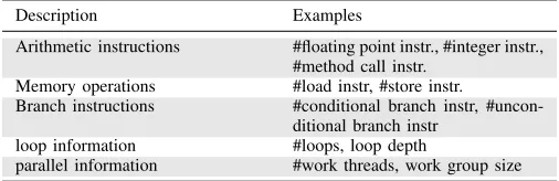
TABLE III: Example code features used in prior works.

Description Examples

Arithmetic instructions #floating point instr., #integer instr., #method call instr.

Memory operations #load instr, #store instr.

Branch instructions #conditional branch instr,

#uncon-ditional branch instr

loop information #loops, loop depth

parallel information #work threads, work group size

One technique that has seen little investigation is the use of Gaussian Processes [112]. Before the recent widespread interest in deep neural networks, these were a highly popular method in many areas of machine learning [113]. They are particular powerful when the amount of training data is sparse and expensive to collect. They also automatically give a confidence interval with any decision. This allows the compiler writer to trade off risk vs reward depending on application scenario,

Using a single model has a significant drawback in practice. This is because a one-size-fits-all model is unlikely to precisely capture behaviors of diverse applications, and no matter how parameterized the model is, it is highly unlikely that a model developed today will always be suited for tomorrow. To allow the model to adapt to the change of the computing environ-ment and workloads, ensemble learning was exploited in prior works [71], [114], [115]. The idea of ensemble learning is to use multiple learning algorithms, where each algorithm is ef-fective for particular problems, to obtain better predictive per-formance than could be obtained from any of the constituent learning algorithm alone [116], [117]. Making a prediction using an ensemble typically requires more computational time than doing that using a single model, so ensembles can be seen as a way to compensate for poor learning algorithms by performing extra computation. To reduce the overhead, fast algorithms such as decision trees are commonly used in ensemble methods (e.g. Random Forests), although slower algorithms can benefit from ensemble techniques as well.

V. FEATUREENGINEERING

Machine learning based code optimisation relies on hav-ing a set of high-quality features that capture the important characteristics of the target program. Given that there is an unbounded number of potential features, finding the right set is a non-trivial task. In this section, we review how previous work chooses features, a task known as feature engineering.

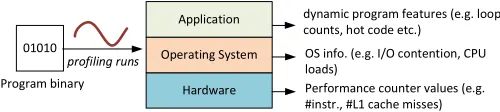
A. Feature representation

Various forms of program features have been used in compiler-based machine learning. These include static code structures [118] and runtime information such as system load [114], [119] and performance counters [51].

01010

Program binary _Hardware

Operating System Application

profiling runs

dynamic program features (e.g. loop counts, hot code etc.)

OS info. (e.g. I/O contention, CPU loads)

Performance counter values (e.g. #instr., #L1 cache misses)

Fig. 12: Dynamic features can be extracted from multiple layers of the computing environment.

Table III gives some of the static code features that were used in previous studies. Raw code features are often used together to create a combined feature. For example, one can divide the number of load instructions by the number of total instructions to get the memory load ratio. An advantage of using static code features is that the features are readily available from the compiler intermediate representation.

2) Other static features: Singer and Veloso represent the

FFT in a split tree [120]. They extract from the tree a set of features, by counting the number of nodes of various types and quantifying the shape of the tree. These tree-based features are then used to build a neural network based cost function that predicts which of the two FFT formulas runs faster. The cost function is used to search for the best-performing transformation.

Parket al.present a unique graph-based approach for feature representations [121]. They use a SVM where the kernel is based on a graph similarity metric. Their technique requires hand coded features at the basic block level, but thereafter, graph similarity against each of the training programs takes the place of global features. Mailike shows that spatial based information, i.e. how instructions are distributed within a program, extracted from the program’s data flow graph could be useful features for machine learning based compiler optimi-sation [122]. Nobreet al.also exploit graph structures for code generation [24]. Their approach targets the phase ordering problem. The order of compiler optimisation passes is repre-sented as a graph. Each node of the graph is an optimisation pass and connections between nodes are weighted in a way that sub-sequences with higher aggregated weights are more likely to lead to faster runtime. The graph is automatically constructed and updated using iterative compilation (where the target program is complied using different compiler passes with different orders). A design space exploration algorithm is employed to drive the iterative compilation process.

3) Dynamic Features: While static code features are useful and can be extracted at static compile time (hence feature extraction has no runtime overhead), they have drawbacks. For examples, static code features may contain information of code segments that rarely get executed, and such in-formation can confuse the machine learning model; some program information such as the loop bound depends on the program input, which can only obtained during execution time; and static code features often may not precisely capture the application behaviour in the runtime environment (such as resource contention and I/O behaviour) as such behaviour highly depends on the computing environment such as the number of available processors and co-running workloads.

As illustrated in Figure 12, dynamic features can be

ex-tracted from multiple layers of the runtime environment. At the application layer, we can obtain information like loop iter-ation counts the cannot be decided at compile time, dynamic control flows, frequently executed code regions, etc. At the operating system level, we can observe the memory and I/O behaviour of the application as well as CPU load and thread contention, etc. At the hardware level, we can use performance counters to track information like how many instructions have been executed and of what types, and the number of cache loads/stores as well as branch misses, etc.

Hardware performance counter values like executed in-struction counts and cache miss rate are therefore used to understand the application’s dynamic behaviours [51], [123]. These counters can capture low-level program information such as data access patterns, branches and computational instructions. One of the advantage of performance counters is that they capture how the target program behave on a specific hardware and avoid the irrelevant information that static code features may bring in. In addition to hardware performance counters, operating system level metrics like system load and I/O contention are also used to model an application’s behavior [37], [119]. Such information can be externally observed without instrumenting the code, and can be obtain during off-line profiling or program execution time. While effective, collecting dynamic information could incur prohibitively overhead and the collected information can be noisy due to competing workloads and operating system scheduling [124] or even subtle settings of the execution environment [125]. Another drawback of performance coun-ters and dynamic features is that they can only capture the application’s past behavior. Therefore, if the application behaves significantly different in the future due to the change of program phases or inputs, then the prediction will be drawn on an unreliable observation. As such, dynamic and static features are often used in combination in prior works in order to build a robust model.

B. Reaction based features

Cavazoset al.present a reaction-based predictive model for software-hardware co-design [126]. Their approach profiles the target program using several carefully selected compiler options to see how program runtime changes under these options for a given micro-architecture setting. They then use the program “reactions” to predict the best available applica-tion speedup. Figure 13 illustrates the difference between a reaction-based model and a standard program feature based model. A similar reaction-based approach is used in [127] to predict speedup and energy efficiency for an application that is parallelised thread-level speculation (TLS) under a given micro-architectural configuration. Note that while a reaction-based approach does not use static code features, developers must carefully select a few settings from a large number of candidate options for profiling, because poorly chosen options can significantly affect the quality of the model.

C. Automatic feature generation

PROCEEDINGS OF IEEE 13

Program source

Candiate compiler

transformation Transformed code

Static program features

Pre

dic

tive

M

od

el

Predicted speedup

Program source

Ha

rdw

are

...

... ...

...

t1

t2

t3

s1 s2 s3 Measured speedups

(reactions)

Pre

dic

tiv

e M

od

el

Predicted speedup

... (010000111000)

Candidate compiler transformation (a) Static program feature based predictor

Program source

Ha

rdw

are

... ...

... t1

t2

t3

s1

s2 s3 Measured speedups

(reactions)

Pre

dic

tiv

e M

od

el

Predicted speedup ...

(010000111000)

Candidate compiler transformation

Selected compiler transforms (t1, t2, t3)

(b) Reaction based predictor

Fig. 13: Standard feature-based modeling (a) vs reaction-based modeling (b). Both models try to predict the speedup for a given compiler transformation sequence. The program feature based predictor takes in static program features extracted from the transformed program, while the reaction based model takes in the target transformation sequence and the measured speedups of the target program, obtained by applying a number of carefully selected transformation sequences. Diagrams are reproduced from [126].

from the compiler’s intermediate representation (IR) [128], [68]. The work of [68] uses GP to search for features, but required a huge grammar to be written, some 160kB in length. Although much of this can be created from templates, selecting the right range of capabilities and search space bias is non triv-ial and up to the expert. The work of [128] expresses the space of features via logic programming over relations that represent information from the IRs. It greedily searches for expressions that represent good features. However, their approach relies on expert selected relations, combinators and constraints to work. Both approaches closely tie the implementation of the predictive model to the compiler IR, which means changes to the IR will require modifications to the model. Furthermore, the time spent in searching features could be significant for these approaches.

The first work to employ neural network to extract fea-tures from program source code for compiler optimisation is conducted by Cummin et al. [76]. Their system, name-ly DeepTune, automaticalname-ly abstracts and selects appropriate features from the raw source code. Unlike prior work where the predictive model takes in a set of human-crafted features, program code is used directly in the training data. Programs are fed through a series of neural network based language models which learn how code correlates with the desired optimisation options (see also Figure 8). Their work also shows that the properties of the raw code that are abstracted by the top layers of the neural networks are mostly independent of the optimisation problem. While promising, it is worth

men-tioning that dynamic information such as the program input size and performance counter values are often essential for characterising the behaviour of the target program. Therefore, DeepTune does not completely remove human involvement for feature engineering when static code features are insufficient for the optimisation problem.

D. Feature selection and dimension reduction

Machine learning uses features to capture the essential characteristics of a training example. Sometimes we have too many features. As the number of features increase so does the number of training examples needed to build an accurate model [129]. Hence, we need to limit the dimension of the feature space In compiler research, commonly, an initial large, high dimensional candidate feature space is pruned via feature selection [50], or projected into a lower dimensional space [15]. In this subsection, we review a number of feature selection and dimension reduction methods.

1) Feature selection: Feature selection requires understand-ing how does a particular feature affect the prediction accuracy. One of the simplest methods for doing this is applying the Pearson correlation coefficient. This metric measures the linear correlation between two variables and is used in numerous works [130], [53], [118], [90] to filter out redundant features by removing features that have a strong correlation with an already selected feature. It has also been used to quantify the relation of the select features in regression. One obvious drawback of using Pearson correlation as a feature ranking mechanism is that it is only sensitive to a linear relationship. Another approach for correlation estimation is mutual infor-mation [126], [131], which quantifies how much inforinfor-mation of one variable (or feature) can be obtained through another variable (feature). Like correlation coefficient, mutual informa-tion can be used to remove redundant features. For example, if the information of feature,x, can be largely obtained through another existing feature, y, feature x can then be taken out from the feature set without losing much information on the reduced feature set.

Both correlation coefficient and mutual information evaluate each feature independently with respect to the prediction. A different approach is to utilise regression analysis for feature ranking. The underlying principal of regression analysis is that if the prediction is the outcome of regression model based on the features, then the most important features should have the highest weights (or coefficients) in the model, while features uncorrelated with the output variables should have weights close to zero. For example, LASSO (least absolute shrinkage and selection operator) regression analysis is used in [132] to remove less useful features to build a compiler-based model to predict performance. LASSO has also been used for feature selection to tune the compiler heuristics for the TRIPS processor [133].