Original citation:
Gu, Chen, Bradbury, Matthew S., Kirton, Jack and Jhumka, Arshad (2018) A decision
theoretic framework for selecting source location privacy aware routing protocols in wireless
sensor networks. Future Generation Computer Systems, 87 . pp. 514-526.
doi:10.1016/j.future.2018.01.046
Permanent WRAP URL:
http://wrap.warwick.ac.uk/103851
Copyright and reuse:
The Warwick Research Archive Portal (WRAP) makes this work by researchers of the
University of Warwick available open access under the following conditions. Copyright ©
and all moral rights to the version of the paper presented here belong to the individual
author(s) and/or other copyright owners. To the extent reasonable and practicable the
material made available in WRAP has been checked for eligibility before being made
available.
Copies of full items can be used for personal research or study, educational, or not-for-profit
purposes without prior permission or charge. Provided that the authors, title and full
bibliographic details are credited, a hyperlink and/or URL is given for the original metadata
page and the content is not changed in any way.
Publisher’s statement:
© 2018. This manuscript version is made available under the CC-BY-NC-ND 4.0 license
http://creativecommons.org/licenses/by-nc-nd/4.0/
A note on versions:
The version presented here may differ from the published version or, version of record, if
you wish to cite this item you are advised to consult the publisher’s version. Please see the
‘permanent WRAP URL’ above for details on accessing the published version and note that
access may require a subscription.
A Decision Theoretic Framework for Selecting Source
Location Privacy Aware Routing Protocols in Wireless
Sensor Networks
Chen Gua,∗, Matthew Bradburya, Jack Kirtona, Arshad Jhumkaa
aDepartment of Computer Science, University of Warwick,
Coventry, CV4 7AL, United Kingdom
Abstract
Source location privacy (SLP) is becoming an important property for a large class of security-critical wireless sensor network applications such as monitoring and tracking. Many routing protocols have been proposed that provide SLP, all of which provide a trade-off between SLP and energy. Experiments have been conducted to gauge the performance of the proposed protocols under different network parameters such as noise levels. As that there exists a plethora of protocols which contain a set of possibly conflicting performance attributes, it is difficult to select the SLP protocol that will provide the best trade-offs across them for a given application with specific requirements. In this paper, we propose a methodology where SLP protocols are first profiled to capture their performance under various protocol configurations. Then, we present a novel decision theoretic procedure for selecting the most appropriate SLP routing algorithm for the application and network under investigation. We show the viability of our approach through different case studies.
Keywords: Source Location Privacy, Wireless Sensor Networks, Decision Theory, Technique Comparison
1. Introduction
A wireless sensor network (WSN) consists of a number of tiny devices, known as sensor nodes or motes, that can sense different attributes of the environment and use radio signals to communicate among themselves. WSNs have enabled the de-velopment of many novel applications, including asset monitoring, target tracking and environment control [1] among others, with low levels of intrusiveness. They are also expected to be deployed in safety and security-critical systems, including
∗Corresponding author
Email addresses: [email protected](Chen Gu),[email protected]
(Matthew Bradbury),[email protected](Jack Kirton),[email protected]
military [2] and medical services. The communication protocols used in the WSNs must therefore meet a set of stringent security and privacy requirements dependent on the application.
Threats to privacy in monitoring applications can be considered along two dimensions: (i) content-based threats and (ii) context-based threats [3]. Content-based privacy threats relate to use of the content of the messages broadcast by sensor nodes, such as gaining the ability to read an eavesdropped encrypted message. There has been much research addressing the issue of providing content privacy, e.g., SPINS [4], with most efforts in this area focusing on the use of cryptographic techniques. On the other hand, context-based privacy threats focus on the context in which messages are broadcast and how information can be observed or inferred by attackers. Context is a multi-attribute concept that encompasses situational aspects of broadcast messages, including environmental and temporal information.
It is often desirable for the source of sensed information to be kept private in a WSN. For example, in a military application, a soldier transmitting messages can unintentionally disclose their location, even when encryption is used. Another example is during the monitoring of endangered species where poachers may be tempted to infer the location of the animal to capture it. Real world examples include monitoring badgers [5] and the WWF’s Wildlife Crime Technology Report [6], both of which would likely benefit from a context-based security measure. In this paper, the context we focus on protecting is thesource location. Techniques that protect this source location are said to provide source location privacy (SLP). SLP is important in many application domains, though it is of utmost concern in security-critical situations. In each of these scenarios, it is important to ensure that an attacker cannot find or deduce the location of the asset being monitored, whether it is a soldier or an endangered animal. A WSN designed to forward the information collected about an asset would typically consist of the following: a dedicated node for data collection called asink node, the node(s) involved in sending information about these assets called source nodes, and many other nodes in the network used to route/relay messages over multiple hops from the sources to the sink. It has been shown that even a weak attacker such as a distributed eavesdropping attacker can backtrack along message paths through the network to find the source node and capture the asset [7]. Thus, there is a need to develop SLP-aware algorithms.
various case studies and show how the suitability of different SLP protocols vary according to the application under study.
Thus, the main contributions of this paper are:
• We propose a 2-step methodology for SLP-aware protocol selection: (i) profiling of protocols and (ii) selection of a protocol.
• The protocol selection step is based on a decision theoretic procedure that first removes dominated protocols and then formalizes the notion of relevance using suitable utility functions.
• We show, through the use of various case studies, the impact that the application has on the suitability of the SLP protocols.
The remainder of this paper is organised as follows: Section 2 surveys related work in SLP and Section 3 presents the models assumed. We present the relevant routing protocols we consider in this paper in Section 4. In Section 5, we present the decision theoretic procedure for selecting the most appropriate SLP-aware routing algorithm. The adopted system and simulation approach are outlined in Section 6. In Section 7 we present an example of the execution of the decision theoretic procedure. Section 8 presents three case studies to showcase the viability of the approach. Section 9 concludes this paper with a summary of contributions.
2. Related Work
2.1. Overview
The concept of the SLP problem was first posed around 2004 in [12] which proposed the panda-hunter game where the poachers only used network traffic flow to track the panda. Kamat formalised the SLP issue based on the panda-hunter game [7]. Since then, several techniques have been proposed to address SLP. The solution spectrum spans from simple solutions such as simple random walk [12] to more sophisticated techniques such as fake sources and diversionary routing in [10, 13, 14, 15].
2.2. Phantom Walk Technique
For other random walk algorithms, an improvement of the directed random walk was introduced in [19], with the introduction of the self-adjusting directed random walk (SADRW). The neighbours were divided into four different sets, and nodes randomly pick a neighbour out of one of the four directional sets and send the messages to it. A new algorithm using location angles was proposed to construct the random walk based on the inclination angle between a node and its neighbour towards the sink [20]. The author Xi introduced the greedy random walk (GROW) [21]. In GROW, one random walk starts from the sink and goes to a randomly chosen receptor-node. The other random walk starts from the source and meets the first random walk at the receptor-node. Then, the receptor-node uses the path established by the random walk from the sink to the receptor-node to route the packet from the source to the sink. Besides, the authors used a different approach, by recording neighbours in a bloom filter which informed the choice of the next node to be used in the random walk [21]. However, there is still scope to improve the nodes that are allocated to take part in the directed random walk. Other algorithms use the random walk technique to address the SLP issue such as randomly selected intermediary node (RRIN) [22], random routing scheme (RRS) [23] and phantom walkabouts [24].
2.3. Fake Source Technique
Algorithms utilise dummy messages sent by afake source to provide SLP. Some nodes are chosen as fake sources and periodically send dummy messages to obfuscate the real traffic. In the early stages, the author Ozturk introduced a concept of fake sources and propose a theoretical algorithm called short-lived fake source routing (SLFSR) [12]. Later on, many algorithms have been proposed with state-of-the-art fake message techniques [10, 25, 26, 27, 28]. These algorithms based on the fake source mentioned so far can only provide SLP against the local attacker.
For the scope of the global attacker, a global protection scheme called Periodic was developed in which every node sends a message after a fixed period [29]. This provided perfect protection against an attacker with a global view of the network. The authors created a model involving traces of source detection, which was used to measure the privacy of those traces as well as the energy cost of providing SLP. In addition, a different approach where statistical techniques were used to show that their global protection scheme provided high levels of SLP [14]. This approach did not provide perfect global SLP as [29] did, but instead provided statistically strong SLP. Their model and solution aimed to make the distribution of message broadcasts from nodes indistinguishable from a certain statistical distribution.
Perhaps the most significant disadvantage of the described fake source tech-niques is the volume of messages broadcast to provide SLP. This leads to increased energy consumption and an increased number of collisions, both of which result in a decreased packet delivery ratio. This means that a tradeoff between energy expenditure and privacy must be made [26], making dummy message schemes challenging for many large-scale networks.
2.4. Other Techniques
Apart from techniques described above, an algorithm was proposed where nodes changed the chronological order of received messages and sent messages which also change the traffic pattern, making it hard for a local adversary to track the traffic to the source node [8]. Wang used separate path routing to transmit messages, leading to less packets per path, making it harder for the adversary to track messages back to the real source [16]. Mules-saving-source protocol (MussP) useα-angle anonymity to provide SLP by adopting data mules which collect the packets from sources and drop them elsewhere [32]. Others include using geographic routing [17] and network coding [33, 34] to address the SLP issue.
3. Models
In this section, we present the various models that underpin this work.
3.1. Network Model
We assume a wireless sensor network to contain a set of resource-constrained nodes that communicate among themselves using radio. When a node senses the environment, it generates a message and sends the message towards a dedicated node called the sink. There are several potential routing algorithms for WSNs. We assume all the nodes to be static, i.e., the topology of the network remains constant as well as the neighbourhoods of all the nodes over the lifetime of the network. We do not assume that links are bidirectional, i.e., links may disappear intermittently.
3.2. Attacker Model
4. Routing Protocols Review
In this section, we will review the SLP-aware routing protocols that will be analysed in this paper. However, the framework we propose can be extended to handle any other SLP-aware routing protocol.
4.1. Protectionless Flooding and Protectionless CTP
Two routing algorithms that provideno SLP will be evaluated in this work to compare against the SLP techniques. The first is flooding in which a source floods a message through the network, by having each node that receives it forwarding it. Flooding is included as it was shown by the seminal work to provide no SLP [7]. The second is CTP [37] (the Collection Tree Protocol) which uses the expected number of transmissions to gauge the reliability of a link to form a routing tree from every node in the network to the sink. CTP is included as it is the state-of-the-art reliable routing protocol for WSNs. No work thus far has analysed its ability to provide SLP.
4.2. Phantom Walkabouts
Phantom walkabouts is an algorithm using a random walk technique to provide SLP [24]. The new technique, which uses a mix of short and long random walks, achieves a higher level of SLP than phantom routing with a bounded message overhead. Authors denote a phantom walkabouts parameterisation by
P W(ms, ml), where msandml denote the number of short and long random
walks respectively to be performed in a cycle. When a source node routes a messageM using phantom walkabouts, a decision is needed regarding whether
M goes on a short or long random route. The sequencing of messages is as follows:
Ms,· · ·, Ms,
| {z }
ms
Ml,· · ·, Ml,
| {z }
ml
Ms,· · · , Ms,
| {z }
ms
Ml,· · ·, Ml,
| {z }
ml
· · ·
For instance, P W(1,1) denotes a repeating sequence of 1 short random walk followed by 1 long random walk. Therefore, we observe that phantom walkabouts consists of ms messages on short random walk Ms and ml messages on long
random walkMl, before the cycle is repeated.
4.3. DynamicSPR
4.4. ILP Routing
In ILP Routing [39], the problem of SLP-aware routing of messages from a source to a sink was modelled as an Integer Linear Programming (ILP) optimisation problem. Using an ILP solver an optimal solution was obtained when trying to maximise the attacker’s distance from the source. As the optimal solution required global knowledge, the authors implemented a distributed version that had a message take a directed walk around the sink to approach it from a direction other than the one the source was in. Messages were delayed by different amounts such that they reached a similar point at a certain distance. By doing this the attacker makes less progress, due to messages being grouped at a similar location and also because messages would be missed that take a different path.
5. Decision Theoretic Procedure for Selecting Routing Algorithm
Given the number of SLP-aware routing protocols, each one optimizing one or more attributes, it becomes challenging to select a protocol for a given application. For example, if an application requires a high level of privacy and is supposed to run for a short time, selecting a protocol that trades-off privacy for lower energy consumption will not be suitable. Thus, there is a need to develop a framework that can guide a network or application designer in selecting the appropriate SLP-aware routing protocol.
In this section, we are thus concerned about structuring the preferences to simplify the trade-off analysis. As we are concerned about multi-attribute optimization, we provide a brief overview of the theory underpinning generation of multi-attribute utility functions. Table 1 summarises the most commonly used symbols in the paper.
5.1. Brief Introduction to Decision Theory (DT)
We refer the readers to [40, 41] for details about multi-objective optimization. Very often, real-world cases deal with more than three attributes. We assume that we have n evaluators, E1, E2, . . . En, evaluating attributes a1, a2, . . . an
respectively, such that (E1(a1), E2(a2), . . . En(an)) = (q1, q2, . . . , qn), where each
qi captures the “performance” of the protocol for a particular attribute and
the vector (q1, q2, . . . , qn) is the “performance” vector of a protocol. An overall
relevance function,G, may be expressed in additive form
G(q1, q2, . . . , qn) = n
X
i=1
(λi∗Gi(qi)) (1)
where Gi’s are single-attribute or individual relevance functions [40, 41], and
Pn
i=1λi= 1 iff the attributes aremutually preferentially independent, i.e.,
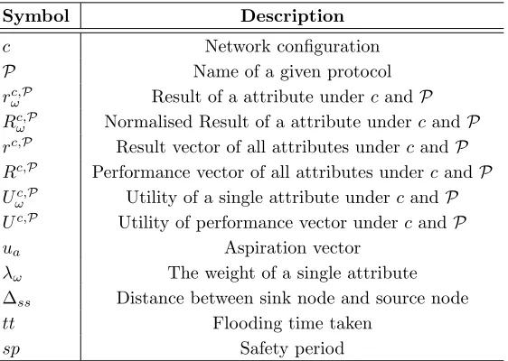
Table 1: Commonly used symbols
Symbol Description
c Network configuration
P Name of a given protocol
rc,P
ω Result of a attribute undercandP
Rc,P
ω Normalised Result of a attribute underc andP
rc,P Result vector of all attributes underc andP Rc,P Performance vector of all attributes underc andP Uωc,P Utility of a single attribute underc andP Uc,P Utility of performance vector undercandP
ua Aspiration vector
λω The weight of a single attribute
∆ss Distance between sink node and source node
tt Flooding time taken
sp Safety period
A higher value ofλi is indicative of a higher importance of the corresponding
attribute. Thus, to generate the overall relevance function, each λi needs to
be determined, subject to the constraintPn
i=1λi = 1. Also, each individual
relevance function Gi needs to be generated by the system administrator or
application developer. Determining an accurateGi is a challenging process. We
direct the interested reader to [40, 41] for more information about generating such functions, which is however beyond the objective of the paper. We will use
arbitrary functions to showcase the decision theoretic methodology we propose in the paper.
5.2. Decision Theory-Based Heuristic
In this section, we present a novel two-step decision procedure (or heuristic) that helps choose the most suitable SLP-aware routing algorithm from a set of contenders for a given application:
Step 1 - Profiling and Filtering
1. For various network configurations (size, safety factor, noise models etc), run all the protocols to obtain their respective performance profiles, i.e., generate their performance vectors. This step can be done once and the profiles stored in a database or library.
there is no profile associated with the input configuration, then either the protocol has to be run under this new configuration (and added to the library) or a profile exists in the library for a configuration that is close enough to the input configuration.
3. For a given input network configuration, determine a vector that best represents the application’s requirements, i.e, determine a vector that captures the acceptable value boundary for each attribute. The boundary is the maximal or minimal acceptable value, depending on the attribute type. We refer to this vector as theaspiration vector.
4. For the given input network configuration, remove all vectors that are either dominated by the aspiration vector (i.e., all entries in the aspiration vector are better than the corresponding ones in the vector under consider-ation), since they fall short of the application’s requirements for the input configuration.
5. If there are no candidates left, go to 3. Else, for each attribute, determine the minimum and maximum values from the remaining alternatives. This is done to help in determining normalized single-attribute functions (range from 0 to 1).
Step 2 - Characterization and Selection
1. Determine the (i) individual weights (or importance) of each attribute, (ii) individual relevance function and (iii) the overall relevance function. 2. For each algorithm (i.e., performance vector) in the set of remaining
contenders, insert the attribute values in the overall relevance function to obtain their respective relevance or utility values.
3. Select the alternative with the highest relevance value.
We now explain the steps in more detail.
5.3. Step 1: Profiling and Filtering SLP-Aware Routing Algorithms
5.3.1. Profiling the Protocols
In the first phase of Step 1, we run every protocol under consideration under various network configurations. These profiles (or protocol performance vectors) can then be saved or stored in a protocol library that can be used whenever a new application is developed. This step need not be repeated for every application, but is a one-time activity. If a new protocol is developed, then the process is repeated for the new protocol, and its (normalized) performance profile is added to the library.
5.3.2. Determining Decision Attributes
We determine four decision attributes that could be classified intogain type (high value is better, e.g., delivery ratio) andcost type (high value is worse, e.g.,
• Capture Ratio (cr) is defined as the number of experiments ending in a capture of attacker in the safety period divided by the total number of experiment repeats for a specific parameter combination. The lower capture ratio is, the higher the source location privacy.
• Delivery Ratio (dr) is defined as the average percentage of messages send by the source that arrive at the sink across multiple simulation repeats.
• Message Latency (lat) is the average amount of time it takes a message to travel from the source to the sink.
• Message Transmission (msg) is the average number of messages transmit-ted through each node per second in the network. The attribute approxi-mates the energy cost as sending and receiving are expensive activities in WSNs [1].
For a given network configurationcand given protocolP, the result vector
rc,P can be determined experimentally (e.g., through simulations). The vector contains the recorded (raw) values of all decision attributes.
rc,P = (rc,crP, r c,P
dr , r c,P
lat, r c,P
msg) (2)
Please note that, since our focus in this paper has been for SLP-awareness, the attributes of interest capture both SLP levels and WSNs performance (e.g., capture ratio, delivery ratio) and these are used in the vector. However, we conjecture that a similar heuristic can be used but for different objectives, requiring a different set of attributes.
An example of a result vector for an arbitrary SLP-aware protocolP0 for an input configurationc0, using the above attributes, could be:
rc0,P0 = (10%,90%,2500,12800) (3)
However, these attributes do not satisfy the mutually preferentially indepen-dent property. This is apparent as, for example, the capture ratio attribute is dependent on the delivery ratio attribute. For example, a low delivery ratio will imply a low capture ratio because the attacker will have overheard only a few messages and would not have been able to track the asset down. In a similar way, message transmission attribute is related to the delivery ratio in that, if a node does not receive a normal (data) message, then it is not going to forward it, reducing the number of message transmissions.
as follows:
Rc,ωP =
rωc,P/r
c,P
dr ifω∈ {cr, msg},
rωc,P otherwise.
(4)
5.3.3. Determining Aspiration Vector
With consideration of different scenarios, we choose the aspiration value for each attribute to remove any results not in the scope to meet the scenario requirement. The aspiration value defines the minimal (or maximal in the case of cost criterion) acceptable value for each attribute. We will denote the aspiration vector byµa.
5.3.4. Filtering the Protocols
Based on the performances of the various protocols, it is obvious that those protocols that are worse (in all attributes) than all other protocols can be removed from the list as it implies that such protocols will never get selected as there is always another protocol that can deliver better result. In our case, based on the selection of protocols that we have chosen, none of them is dominated and thus none of them gets removed from the list. For example,ILP Routing-Max
has very low capture ratio but has very high latency as its mechanism is based on using time redundancy to achieve privacy.
5.3.5. Checking Remaining Values
For each attribute, we check whether any results are left in the scope of the aspiration value. If not, return to phase 3 and reselect the aspiration value as all remaining results do not satisfy the aspiration value.
5.4. Step 2: Characterization and Selection of SLP-Aware Routing Algorithms
5.4.1. Determining Weights and Utility Functions
In the first phase of step 2, we choose individual weightλω(ω∈ {cr, dr, lat, msg})
which represents the importance of attributes. From step 1, having the aspiration vector, we use it to generate the utility function for each attribute. The total utility obtained by some algorithm is shown below, whereUc,P
ω is single attribute
utility andRc,P
ω is a result value inRc,P.
Uc,P(λω, Rωc,P) =
X
λω·Uωc,P(R c,P
ω ) (5)
5.4.2. Inserting Attribute Values
In the second phase of step 2, for each attribute, we use utility functions and the remaining normalised result vector (i.e., performance vector) in the library as input to calculate the utility value. Then the final utility of algorithm under
5.4.3. Selecting Utility Value
After proceeding above, we have obtained utility values of all algorithms and have choosen the best algorithm in terms of the highest utility value. In this case, we claim that under network configurationcand the given scenario, the algorithm with the highest utility value has the best performance.
6. Experimental Setup
In this section, we describe the simulation setup, parameters setup and safety period calculation that were used to generate the results (i.e., performance library), presented in Section 8.
6.1. Simulation Setup
The TOSSIM (V2.1.2) simulation environment was used in all experiments [42]. TOSSIM is a discrete event simulator capable of accurately modelling sensor nodes and the modes of communications between them. An experiment is made of a single execution of the simulation environment using a specified protocol configuration, network nodes and safety period. An experiment terminated when any source node had been captured by an attacker during the safety period or the safety period had expired.1
6.2. Parameters Setup
A square grid network layout of sizen×n was used in all experiments, with
n∈ {11,21}, i.e., networks with 121 and 441 nodes respectively. Source node generated messages and a single sink node collected messages. These nodes were assigned positions in theSourceCorner configuration from [10] where the source is in the corner and sink at the center of the grid. The rate at which messages from the real sources was generated was set to be 1 message per second. Nodes were placed 4.5 meters apart. At least 2000 repeats were performed for each combination of source location and parameters.
The node neighbourhoods were generated using two types of radio models. The first is ideal, which is a unit disk graph radio model (UDGM) where a perfectly reliable network link exists between the edges of a node’s neighbours that are 4.5 meters away. The second is low-asymmetry, which uses the LinkLay-erModel tool provided with TOSSIM to generate link strengths between nodes using the parameters shown in Table 3. Links generated with low-asymmetry have a small probability of becoming asynchronous.
The noise model was created using the first 2500 lines ofcasino-lab.txt and
meyer-heavy.txt2. All the nodes are stationary (i.e., they do not move in the
network).
1The source code for the algorithms tested and the scripts to run the experiments are
available athttps://bitbucket.org/Chen_Gu/slp-algorithms-tinyos.
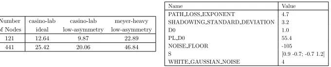
Number casino-lab casino-lab meyer-heavy of Nodes ideal low-asymmetry low-asymmetry
[image:14.612.140.480.123.192.2]121 12.64 9.87 22.89 441 25.42 20.06 46.84
Table 2: Time Taken for each network size when one message is sent per second.
Name Value
PATH LOSS EXPONENT 4.7 SHADOWING STANDARD DEVIATION 3.2
D0 1.0
PL D0 55.4
NOISE FLOOR -105
S [0.9 -0.7; -0.7 1.2]
WHITE GAUSSIAN NOISE 4
Table 3: LinkLayerModel Parameters for the low-asymmetry radio model
6.2.1. Phantom Routing and Phantom Walkabouts
These two algorithms both rely on the random walk technique. When choos-ing the length of the short and long random walks, a variety of parameter combinations were considered. Our experiments set the short random walk seriesS={2,3, . . . ,0.5×∆ss}, and long random walk seriesL={2 + ∆ss,3 +
∆ss, . . . ,1.5×∆ss}, where ∆ss is the sink source distance. In the phantom
walkabouts, the short and long random walk length are randomly generated fromS andLrespectively. For phantom routing, we fix random walk length to be 0.5×∆ss hops.
6.2.2. DynamicSPR
For this technique, as it aims to dynamically determine the parameters to use online, there are few parameters to specify. Other than the previously mentioned parameters, only the approach used needs to be specified. The approach determines how many fake messages are sent over the lifetime of a temporary fake source. There are three options: Fixed1, Fixed2 andRnd.
Fixed1sends a single fake message over the duration, Fixed2sends two fake
messages over the duration and Rnd sends either 1 or 2 messages randomly chosen.
6.2.3. ILP Routing
This algorithm has four parameters: the maximum walk length, the buffer size, the number of messages to group and the probability the message is sent directly to the sink. We use the same parameters as used in [39]. As the maximum walk length is simply to provide a finite bound in large networks, it was set to 100 hops. The number of messages to group was varied between{1, 2, 3, 4}. The buffer size was set to 10 messages as we do not expect more than 10 concurrent messages being sent in the network at one time. Finally, the probability of sending a message directly to the sink was set to 20% as it was identified as a good setting in the paper.
6.2.4. Protectionless Routing
such as neighborhood information, to keep the routing reliable, the attacker cannot make use of this information as the relevance is only local. On the other hand, capturing a source required global information about the network.
6.3. Safety Period
A metric called thesafety period (which we calltime-to-capture from this point) was introduced in [7] which is the number of messages sent that an attacker needs to capture the source. The higher the time-to-capture is, the higher the source location privacy level. Using the time-to-capture metric means that simulation runtime is unbounded and potentially very large.
We thus use an alternative, but analogous, definition for safety period for each network size and network topology, we obtain the time-to-capture when protectionless flooding is used as the routing protocol. Flooding is used as it has been argued to provide the least SLP level, hence any SLP improvement is due to the SLP-aware technique [7]. The safety period is then obtained by increasing this value to account for the attacker potentially making bad moves. This definition is commensurate with [10, 26, 27, 35], but uses a different multiplicative factor due to the difference in the type of SLP technique being used.
Intuitively, the safety period captures the time period during which the asset will be at the same location. We calculate different safety periods spas the following, wherettis the time-to-capture for protectionless flooding andψis the safety factor.
sp=ψ×tt ψ∈ {0.4,0.8,1.2, . . . ,2.8} (6)
The time takenttfor each network size and network topology, for protection-less flooding is shown in table Table 2.
7. Example Execution of Decision Theoretic Procedure
In this section, we provide a brief example of the execution of the decision theoretic procedures we proposed during theprofiling and filtering phase (Sub-section 5.3) and theselection phase (Subsection 5.4).
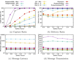
Figure 1 is an example containing the results of the capture ratio, delivery ratio, latency and message transmission for the various protocols under consid-eration, with network configurationc= (grid, 121, SourceCorner, CasinoLab, LowAsymmetry, 1.2) which specifies that the network is a grid network of 121 nodes (i.e., 11*11),SourceCorner topology (the source is at one corner of the grid), Casino Lab noise model, Low Asymmetry communication model and 1.2×tt safety period respectively. From Table 2, we can calculate that the actual safety period is 11.84 seconds. For simplicity, we only evaluate the overall utility of phantom routing and P W(1,1) for comparison for such a network configuration.
7.1. Step 1: Profiling and Filtering SLP-Aware Routing Algorithms
AdaptiveSPR - Max AdaptiveSPR - Min ILP - Max
ILP - Min PW (1, 1) PW (1, 2)
Phantom Protectionless ProtectionlessCTP 0 20 40 60 80 100
0.4 0.8 1.2 1.6 2 2.4 2.8
C a p tu re R a ti o ( % ) Safety Factor
(a) Capture Ratio
0 20 40 60 80 100
0.4 0.8 1.2 1.6 2 2.4 2.8
D e liv e ry R a ti o ( % ) Safety Factor
(b) Delivery Ratio
10 100 1000 10000
0.4 0.8 1.2 1.6 2 2.4 2.8
M e ss a g e L a te n cy ( m s) Safety Factor
(c) Message Latency
0 50 100 150 200 250 300 350 400 450
0.4 0.8 1.2 1.6 2 2.4 2.8
M e ss a g e T ra n sm is si o n ( m e ss a g e s) Safety Factor
[image:16.612.147.462.121.375.2](d) Message Transmission
Figure 1: Example: Multiple Algorithm Results
7.1.1. Profiling the Protocols
We execute a number of routing protocols, as explained in Section 6, some SLP-aware and others not. Figure 1 shows the graphs of capture ratio, delivery ratio, latency and message transmission.
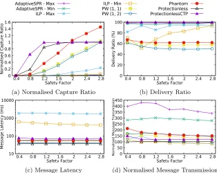
Under configurationc(as above), the result vector of phantom routing is (0.25, 0.65, 0.05, 100), with 25% capture ratio, 65% delivery ratio, 50 ms for latency and 100 messages for message transmission. Similarly, the result vector ofP W(1,1) is (0.1, 0.6, 0.06, 75). As discussed in Subsubsection 5.3.2, results of attributes in the vector are not mutually preferentially independent, so need to be normalised in this case. The normalised results are shown in Figure 2. We calculate the normalised result vector of phantom routing, and is (0.38,0.65,0.05,153.85), while the normalised result vector ofP W(1,1) is (0.17,0.6,0.06,125). We use the normalised result vectors, or performance vectors, to form the protocol performance library, from which the most suitable SLP-aware protocol is to be selected. Since the objective here is to show the execution of our decision theoretic procedure, we focused on phantom routing and PW(1,1) as routing protocols.
7.1.2. Determining Decision Attributes
AdaptiveSPR - Max AdaptiveSPR - Min ILP - Max
ILP - Min PW (1, 1) PW (1, 2)
Phantom Protectionless ProtectionlessCTP 0 0.2 0.4 0.6 0.8 1 1.2 1.4 1.6
0.4 0.8 1.2 1.6 2 2.4 2.8
N o rm a lis e d C a p tu re R a ti o Safety Factor
(a) Normalised Capture Ratio
0 20 40 60 80 100
0.4 0.8 1.2 1.6 2 2.4 2.8
D e liv e ry R a ti o ( % ) Safety Factor
(b) Delivery Ratio
10 100 1000 10000
0.4 0.8 1.2 1.6 2 2.4 2.8
M e ss a g e L a te n cy ( m s) Safety Factor
(c) Message Latency
0 50 100 150 200 250 300 350 400 450
0.4 0.8 1.2 1.6 2 2.4 2.8
N o rm a lis e d M e ss a g e T ra n sm is si o n Safety Factor
[image:17.612.147.461.123.373.2](d) Normalised Message Transmission
Figure 2: Example: Multiple Algorithm Results of Normalised Capture Ratio and Message Transmission
SLP, capture ratio and message or energy overhead are the two most important overhead. However, there are applications when other parameters such as delivery ratio is important. In this paper, for the applications we consider, the above four attributes are considered relevant.
7.1.3. Determining Aspiration Vector
We now determine the aspiration value for each attribute. For instance, if 50% is given as a aspiration value for capture ratio and 60% for delivery ratio, the utility of capture ratio and delivery ratio will be set to 0 at these values. The system designer may consider that SLP cannot be provided if the capture ratio is greater than 50% and that the routing of protocol cannot work properly if the delivery ratio is lower than 60%. In this example, the aspiration vector is set to (0.5,0.5,0.1,250). This means that the normalized capture ratio is set to 50%, the delivery ratio is set to 50%, latency is set at 100 ms and the message overhead at 250.
7.1.4. Filtering the Protocols
the capture ratio and message transmission ofP W(1,1) perform better than phantom routing. Hence, we conclude that PW(1,1) does not dominate phantom routing and vice-versa. Therefore, in this case, we retain both for consideration.
7.1.5. Checking Remaining Values
Since neither PW(1,1) nor phantom routing dominate each other, we need to determine whether they are dominated by the aspiration vector. The aspiration vector is (0.5,0.5,0.1,250) while the performance profiles of phantom routing and PW(1,1) is (0.38,0.65,0.05,153.85) and (0.17,0.6,0.06,125) respectively. As can be observed, the aspiration vector does not dominate either of the protocols, hence both protocols are still under consideration.
7.2. Step 2: Characterization and Selection of algorithms
Since there is more than a single protocol still in contention, i.e., there is no clear winner, we now detail Step 2 to select the better protocol.
7.2.1. Determining Weights and Utility Functions
Based on the aspiration vector, we use sigmoid functions to build the utility functions for attributes3. We choose the parameters and generate the utility functions for the four attributes, as shown in Equation 7 to Equation 10. For simplicity, we adopt a weight vector with equal valuesλ= (0.25,0.25,0.25,0.25), meaning that all four attributes are equally as important.
Ucrc,P(Rc,crP) = 1 1 +e10(Rc,crP−0.5)
(7)
Udrc,P(Rc,drP) = 1
1 +e10(−Rc,drP+0.5) (8) Ulatc,P(Rc,latP) = 1
1 +e2(Rc,latP−1.5) (9) Umsgc,P(Rc,msgP ) = 1
1 +e0.005(Rc,msgP−1000)
(10)
7.2.2. Inserting Attribute Values
Using the utility functions identified (Equation 7 to Equation 10), we can calculate the utility value of each attribute in phantom routing: Uc,P
cr (0.38) = 0.76,
Udrc,P(0.65) = 0.82, Ulatc,P(0.05) = 0.95 andUmsgc,P(153.85) = 0.99. Finally, using the identified weight vectorλ, the final utility of protocolP phantom routing undercis:
Uc,P(λω, Rc,ωP) =
X
λω·Uωc,P(R c,P
ω )
= 0.25×0.76 + 0.25×0.82 + 0.25×0.95 + 0.25×0.99
= 0.88
(11)
Similarly, the utility value ofP W(1,1) also can be calculated: Ucrc,P(0.17) = 0.96, Udrc,P(0.6) = 0.73, Ulatc,P(0.06) = 0.95 and Uc,P
msg(125) = 0.99. The final
utility is 0.91.
7.2.3. Selecting Utility Value
Comparing the final utility of phantom routing andP W(1,1), we selectP W(1,1) as the better algorithm to provide SLP under a network configuration c and with weightλ, as it is the one with the highest utility value.
8. Case Studies: Routing Protocol Selection for Different Application Scenarios
In this section, we will develop three case studies to showcase both the appli-cability of, and the generality allowed by, our methodology. The three case studies we present are : (i) an animal protection scenario, (ii) a non-critical asset monitoring scenario and (iii) a security-critical military scenario.4
In the first phase, we reuse the library that has already been built, that consists of a number of protocols that have been profiled. We denote the library by L and the protocols are listed in Table 4. Next, we identified the set of
decision attributes to consist of (i) capture ratio, (ii) delivery ratio, (iii) latency and (iv) message overhead.
In the next step, rather than deciding on the input network configuration, we will eschew this step so as to keep the discussion as general as possible. We also have the following aspiration vector:
µa= (min{Rc,P
cr | P ∈L},max{R
c,P
dr | P ∈L},min{R
c,P
lat | P ∈L},min{Rc,msgP | P ∈L}) (12)
Thus, this means that all protocols are in contention and will be under consideration, i.e., there is no filtering of protocols at this time.
The first phase of Step 2 is to decide the importance of each of the attributes (from capture ratio, delivery ratio, latency and message transmission) and to create a vector of weights quantifying the preference of each metric. Utilising the data and methods presented in Subsection 5.3, it is possible to calculate the utility of each protocol-parameter combination and generate plots to show which combination provides the highest utility for the given scenario. Specifically, using an input network configurationc, it is possible to then select the most appropriate protocol.
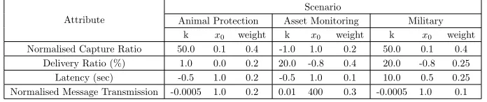
For attributes, we use both non-linear5 and linear functions6to model the
utility of each parameter, as shown in Table 5. For those important attributes, non-linear functions are used to satisfy the quick change rate of utility while linear functions are used for smooth change rate. Parameters for the different attribute utility functions in different scenarios are shown in Table 6.
4The dataset used to generated these results can be found at [43].
5We use sigmoid function with formulaf(x) = 1
1+ek(−x−x0 )
6The formula isf(x) =kx+x
For all case studies, the network is assumed to be a grid with the source node assumed to be at the top-left corner (i.e., a SourceCorner configuration). Note that these need not be the case and there is no constraint imposed by the approach that precludes certain types of networks.
Algorithm Name Technique SLP-aware?
Protectionless Flooding No
Protectionless CTP Collection Tree Protocol No
DynamicSPR Fake Messages Yes
ILP Routing Directed Walk Yes
[image:20.612.156.451.183.289.2]Phantom Routing Directed Random Walk Yes Phantom Walkabouts Directed Random Walk Yes
Table 4: Algorithms Library (L)
Attribute Function Model Types
Animal Protection Asset Monitor Military Normalised Capture Ratio Non-Linear Linear Non-Linear
Delivery Ratio (%) Linear Non-Linear Non-Linear
Latency (sec) Linear Linear Non-Linear
[image:20.612.133.477.331.408.2]Normalised Message Transmission Linear Non-Linear Linear
Table 5: Function Model Types
Attribute
Scenario
Animal Protection Asset Monitoring Military
k x0 weight k x0 weight k x0 weight
Normalised Capture Ratio 50.0 0.1 0.4 -1.0 1.0 0.2 50.0 0.1 0.4
Delivery Ratio (%) 1.0 0.0 0.2 20.0 -0.8 0.4 20.0 -0.8 0.25
Latency (sec) -0.5 1.0 0.2 -0.5 1.0 0.1 10.0 0.5 0.25
Normalised Message Transmission -0.0005 1.0 0.2 0.01 400 0.3 -0.0005 1.0 0.1
Table 6: Parameters for Attribute Utility Functions in Different Scenarios
8.1. Animal Protection Scenario
[image:20.612.131.479.450.523.2]AdaptiveSPR - Max AdaptiveSPR - Min ILP - Max
ILP - Min PW (1, 1) PW (1, 2)
Phantom Protectionless ProtectionlessCTP 0 0.2 0.4 0.6 0.8 1
0.4 0.8 1.2 1.6 2 2.4 2.8
U ti lit y (A n im a l P ro te ct io n ) Safety Factor (a) 121/CasinoLab/Ideal 0 0.2 0.4 0.6 0.8 1
0.4 0.8 1.2 1.6 2 2.4 2.8
U ti lit y (A n im a l P ro te ct io n ) Safety Factor (b) 441/CasinoLab/Ideal 0 0.2 0.4 0.6 0.8 1
0.4 0.8 1.2 1.6 2 2.4 2.8
U ti lit y (A n im a l P ro te ct io n ) Safety Factor (c) 121/CasinoLab/LowAsymmetry 0 0.2 0.4 0.6 0.8 1
0.4 0.8 1.2 1.6 2 2.4 2.8
U ti lit y (A n im a l P ro te ct io n ) Safety Factor (d) 441/CasinoLab/LowAsymmetry 0 0.2 0.4 0.6 0.8 1
0.4 0.8 1.2 1.6 2 2.4 2.8
U ti lit y (A n im a l P ro te ct io n ) Safety Factor (e) 121/MeyerHeavy/LowAsymmetry 0 0.2 0.4 0.6 0.8 1
0.4 0.8 1.2 1.6 2 2.4 2.8
[image:21.612.145.463.122.483.2]U ti lit y (A n im a l P ro te ct io n ) Safety Factor (f) 441/MeyerHeavy/LowAsymmetry
Figure 3: Utility of Animal Protection Scenario
allowing us to deliberate on which protocol and parameter combination would be most suited for the application. Figure 3 shows the overall utility values generated using the weights and utility functions previously specified7.
Protocol Selection: From the utility values, the input network configuration is required. For example, if the animal is expected to trigger a node that is at the top-left corner of a grid network of 11*11 that has been deployed and that the animal is expected to be constantly on the move (i.e., spend only a short time at a given location), and the environment is expected to be lightly noisy (i.e.,
7For simplicity, each configuration was described under corresponding graph with such
similar to the Casino Lab noise model) and the links are expected to be often unidirectional, then the input configuration can be as follows: c= (grid, 121, SourceCorner, CasinoLab, LowAsymmetry, 1.2). Then, this configuration will correspond to Figure 3c and the best protocol is AdaptiveSPR that AdaptiveSPR-Min and AdaptiveSPR-max provide near-comparable performance. On the other hand, for example, if the input configuration isc = (grid, 441, SourceCorner, CasinoLab, Ideal, 1.2), then the protocols that achieve the best trade-offs are PW(1,1) and PW(1,2) (see Figure 3b).
8.2. Asset Monitoring Scenario
Sensors are often deployed in the body of bridges or in a building to monitor product quality [2]. They can also be deployed to monitor and understand animal behaviour (e.g., Great Duck Island [1]), differently from animal protection, as explained in the previous section. For this type of application, it could be assumed that delivery ratio is the most important factor. This would leave capture ratio, latency and message transmission to be less important. Assume the weighting vector λ = (0.2,0.4,0.1,0.3) respectively representing capture ratio, delivery ratio, latency and message transmission.
Protocol Selection: From the utility values, the input network configuration is required. For example, if the animal is expected to trigger a node that is at the top-left corner of a grid network of 11*11 that has been deployed. Since the animal is not expected to be very mobile and the environment can be expected to be noisy (i.e., similar to the Meyer Heavy noise model) with unidirectional links due to a lack of line-of-sight transmission, then the input configuration can be as follows: c = (grid, 121, SourceCorner, MeyerHeavy, LowAsymmetry, 2). Then, this configuration will correspond to Figure 4e and the best protocol is Protectionless CTP.
On the other hand, if the environment is not very noisy, i.e., similar to the Casino Lab noise model, then with a network configurationc = (grid, 121, SourceCorner, CasinoLab, LowAsymmetry, 2), ILP Routing is the protocol that achieves the best trade-off Figure 4c.
8.3. Military Scenario
The use of sensor networks in military situations includes communication, battle-field surveillance and battle damage assessment among many others [2]. When these activities are carried out by military personnel, then SLP is extremely important. Further, these networks may be short-lived, thus message overhead is not very important. On the other hand, latency and delivery ratio are important, though less than SLP, to ensure soldiers can communicate in near real-time. Thus, the weight vector isλ= (0.4,0.25,0.25,0.1).
AdaptiveSPR - Max AdaptiveSPR - Min ILP - Max
ILP - Min PW (1, 1) PW (1, 2)
Phantom Protectionless ProtectionlessCTP 0 0.2 0.4 0.6 0.8 1
0.4 0.8 1.2 1.6 2 2.4 2.8
U ti lit y (A ss e t M o n it o r) Safety Factor (a) 121/CasinoLab/Ideal 0 0.2 0.4 0.6 0.8 1
0.4 0.8 1.2 1.6 2 2.4 2.8
U ti lit y (A ss e t M o n it o r) Safety Factor (b) 441/CasinoLab/Ideal 0 0.2 0.4 0.6 0.8 1
0.4 0.8 1.2 1.6 2 2.4 2.8
U ti lit y (A ss e t M o n it o r) Safety Factor (c) 121/CasinoLab/LowAsymmetry 0 0.2 0.4 0.6 0.8 1
0.4 0.8 1.2 1.6 2 2.4 2.8
U ti lit y (A ss e t M o n it o r) Safety Factor (d) 441/CasinoLab/LowAsymmetry 0 0.2 0.4 0.6 0.8 1
0.4 0.8 1.2 1.6 2 2.4 2.8
U ti lit y (A ss e t M o n it o r) Safety Factor (e) 121/MeyerHeavy/LowAsymmetry 0 0.2 0.4 0.6 0.8 1
0.4 0.8 1.2 1.6 2 2.4 2.8
[image:23.612.144.463.121.483.2]U ti lit y (A ss e t M o n it o r) Safety Factor (f) 441/MeyerHeavy/LowAsymmetry
Figure 4: Utility of Asset Monitoring Scenario
MeyerHeavy noise model) with unidirectional links due to a lack of line-of-sight transmission, then the input configuration can be as follows: c = (grid, 121, SourceCorner, MeyerHeavy, LowAsymmetry, 1.2). Then, this configuration will correspond to Figure 5e and the best protocol is AdaptiveSPR.
On the other hand, if the environment is not very noisy, i.e., similar to the Casino Lab noise model, then with a network configurationc= (grid,441, SourceCorner, CasinoLab, LowAsymmetry, 1.2), AdaptiveSPR is the protocol that achieves the best trade-off in Figure 5d.
AdaptiveSPR - Max AdaptiveSPR - Min ILP - Max
ILP - Min PW (1, 1) PW (1, 2)
Phantom Protectionless ProtectionlessCTP 0 0.2 0.4 0.6 0.8 1
0.4 0.8 1.2 1.6 2 2.4 2.8
U ti lit y (M ili ta ry ) Safety Factor (a) 121/CasinoLab/Ideal 0 0.2 0.4 0.6 0.8 1
0.4 0.8 1.2 1.6 2 2.4 2.8
U ti lit y (M ili ta ry ) Safety Factor (b) 441/CasinoLab/Ideal 0 0.2 0.4 0.6 0.8 1
0.4 0.8 1.2 1.6 2 2.4 2.8
U ti lit y (M ili ta ry ) Safety Factor (c) 121/CasinoLab/LowAsymmetry 0 0.2 0.4 0.6 0.8 1
0.4 0.8 1.2 1.6 2 2.4 2.8
U ti lit y (M ili ta ry ) Safety Factor (d) 441/CasinoLab/LowAsymmetry 0 0.2 0.4 0.6 0.8 1
0.4 0.8 1.2 1.6 2 2.4 2.8
U ti lit y (M ili ta ry ) Safety Factor (e) 121/MeyerHeavy/LowAsymmetry 0 0.2 0.4 0.6 0.8 1
0.4 0.8 1.2 1.6 2 2.4 2.8
[image:24.612.143.463.121.483.2]U ti lit y (M ili ta ry ) Safety Factor (f) 441/MeyerHeavy/LowAsymmetry
Figure 5: Utility of Military Scenario
9. Conclusion and Future Work
In this paper, we propose a decision theoretic procedure for selecting the SLP-aware routing algorithm that achieves the best trade-offs among a set of attributes. The methodology is based on the existence of a library of performance profiles of the various routing algorithms and the decision theoretic procedure allows trade-offs to be assessed. This can be achieved when the attributes are mutually preferentially independent. The utility functions, the weights of the attributes and the network configurations are inputs that have to be provided by network administrators. We have presented three case studies to showcase the viability of the approach.
focus on generating profiles for network configurations where the source is not located in the corner but rather at other locations in the network. We conjecture that specific protocols may have to be developed when the source is located elsewhere than the corner. Secondly, we will consider other protocols, such as OLSR [44], for protectionless routing to provide a baseline profile. And finally, we plan on investigating the suitability of preference learning [45] for selecting appropriate values for aspiration levels.
References
[1] A. Mainwaring, D. Culler, J. Polastre, R. Szewczyk, J. Anderson, Wireless sensor networks for habitat monitoring, in: Proceedings of the 1st ACM International Workshop on Wireless Sensor Networks and Applications, WSNA ’02, ACM, New York, NY, USA, 2002, pp. 88–97. doi:10.1145/
570738.570751.
[2] I. Akyildiz, W. Su, Y. Sankarasubramaniam, E. Cayirci, Wireless sensor networks: a survey, Computer Networks 38 (4) (2002) 393 – 422. doi:
10.1016/S1389-1286(01)00302-4.
[3] J. Lopez, R. Rios, F. Bao, G. Wang, Evolving privacy: From sensors to the internet of things, Future Generation Computer Systems 75 (Supplement C) (2017) 46 – 57. doi:https://doi.org/10.1016/j.future.2017.04.045.
URL http://www.sciencedirect.com/science/article/pii/
S0167739X16306719
[4] A. Perrig, R. Szewczyk, J. D. Tygar, V. Wen, D. E. Culler, Spins: Security protocols for sensor networks, Wirel. Netw. 8 (5) (2002) 521–534. doi:
10.1023/A:1016598314198.
[5] V. Dyo, S. A. Ellwood, D. W. Macdonald, A. Markham, N. Trigoni, R. Wohlers, C. Mascolo, B. P´asztor, S. Scellato, K. Yousef, Wildsens-ing: Design and deployment of a sustainable sensor network for wildlife monitoring, ACM Trans. Sen. Netw. 8 (4) (2012) 29:1–29:33. doi:
10.1145/2240116.2240118.
[6] WWF, Wildlife crime technology project, Online, accessed: 2016-06-03 (2012–2016).
URLworldwildlife.org/projects/wildlife-crime-technology-project
[7] P. Kamat, Y. Zhang, W. Trappe, C. Ozturk, Enhancing source-location privacy in sensor network routing, in: 25th IEEE International Conference
on Distributed Computing Systems (ICDCS’05), 2005, pp. 599–608. doi:
10.1109/ICDCS.2005.31.
[8] X. Hong, P. Wang, J. Kong, Q. Zheng, jun Liu, Effective probabilistic approach protecting sensor traffic, in: Military Communications Conference (MILCOM), 2005 IEEE, 2005, pp. 169–1751. doi:10.1109/MILCOM.2005.
[9] Y. Ouyang, Z. Le, G. Chen, J. Ford, F. Makedon, Entrapping adversaries for source protection in sensor networks, in: International Symposium on a World of Wireless, Mobile and Multimedia Networks, 2006. WoWMoM 2006, 2006, pp. 10–34. doi:10.1109/WOWMOM.2006.40.
[10] A. Jhumka, M. Bradbury, M. Leeke, Fake source-based source location privacy in wireless sensor networks, Concurrency and Computation: Practice and Experience 27 (12) (2015) 2999–3020. doi:10.1002/cpe.3242.
[11] M. Conti, J. Willemsen, B. Crispo, Providing source location privacy in wireless sensor networks: A survey, IEEE Communications Surveys and Tu-torials 15 (3) (2013) 1238–1280. doi:10.1109/SURV.2013.011413.00118.
[12] C. Ozturk, Y. Zhang, W. Trappe, Source-location privacy in energy-constrained sensor network routing, in: Proceedings of the 2nd ACM
workshop on Security of ad hoc and sensor networks, SASN ’04, ACM, New York, NY, USA, 2004, pp. 88–93. doi:10.1145/1029102.1029117.
[13] Y. Yang, M. Shao, S. Zhu, B. Urgaonkar, G. Cao, Towards event source unob-servability with minimum network traffic in sensor networks, in: Proceedings of the First ACM Conference on Wireless Network Security, WiSec ’08, ACM, New York, NY, USA, 2008, pp. 77–88. doi:10.1145/1352533.1352547.
[14] M. Shao, Y. Yang, S. Zhu, G. Cao, Towards statistically strong source anonymity for sensor networks, in: INFOCOM, 2008 Proceedings IEEE, 2008. doi:10.1109/INFOCOM.2008.19.
[15] J. Long, M. Dong, K. Ota, A. Liu, Achieving source location privacy and network lifetime maximization through tree-based diversionary routing in wireless sensor networks, IEEE Access 2 (2014) 633–651. doi:10.1109/
ACCESS.2014.2332817.
[16] H. Wang, B. Sheng, Q. Li, Privacy-aware routing in sensor networks, Com-puter Networks 53 (9) (2009) 1512–1529. doi:10.1016/j.comnet.2009.
02.002.
[17] R. A. Shaikh, H. Jameel, B. J. D’Auriol, H. Lee, S. Lee, Y.-J. Song, Achieving network level privacy in wireless sensor networks, Sensors 10 (3) (2010) 1447–1472. doi:10.3390/s100301447.
[18] L. Lightfoot, Y. Li, J. Ren, Preserving source-location privacy in wireless sensor network using star routing, in: Global Telecommunications Con-ference (GLOBECOM 2010), 2010 IEEE, 2010, pp. 1–5. doi:10.1109/
GLOCOM.2010.5683603.
[19] L. Zhang, A self-adjusting directed random walk approach for enhancing source-location privacy in sensor network routing, in: Proceedings of the 2006 International Conference on Wireless Communications and Mobile Computing, IWCMC ’06, ACM, New York, NY, USA, 2006, pp. 33–38.
[20] W. Wei-Ping, C. Liang, W. Jian-xin, A source-location privacy protocol in wsn based on locational angle, in: Communications, 2008. ICC’08. IEEE International Conference on, IEEE, 2008, pp. 1630–1634.
[21] Y. Xi, L. Schwiebert, W. Shi, Preserving source location privacy in monitoring-based wireless sensor networks, in: 20th International
Paral-lel and Distributed Processing Symposium, 2006, pp. 1–8. doi:10.1109/
IPDPS.2006.1639682.
[22] Y. Li, L. Lightfoot, J. Ren, Routing-based source-location privacy pro-tection in wireless sensor networks, in: IEEE International Conference on Electro/Information Technology, 2009. eit ’09., 2009, pp. 29–34. doi:
10.1109/EIT.2009.5189579.
[23] X. Luo, X. Ji, M.-S. Park, Location privacy against traffic analysis attacks in wireless sensor networks, in: 2010 International Conference on Information Science and Applications (ICISA), 2010, pp. 1–6. doi:10.1109/ICISA.
2010.5480564.
[24] C. Gu, M. Bradbury, A. Jhumka, Phantom walkabouts in wireless sensor networks, in: Proceedings of the Symposium on Applied Computing, SAC’17, ACM, New York, NY, USA, 2017, pp. 609–616. doi:10.1145/3019612.
3019732.
[25] H. Chen, W. Lou, From nowhere to somewhere: Protecting end-to-end location privacy in wireless sensor networks, in: Performance Computing and Communications Conference (IPCCC), 2010 IEEE 29th International,
2010, pp. 1–8. doi:10.1109/PCCC.2010.5682341.
[26] A. Jhumka, M. Leeke, S. Shrestha, On the use of fake sources for source location privacy: Trade-offs between energy and privacy, The Computer Journal 54 (6) (2011) 860–874. doi:10.1093/comjnl/bxr010.
[27] M. Bradbury, M. Leeke, A. Jhumka, A dynamic fake source algorithm for source location privacy in wireless sensor networks, in: 14th IEEE International Conference on Trust, Security and Privacy in Computing and Communications (TrustCom), 2015, pp. 531–538. doi:10.1109/Trustcom.
2015.416.
[28] A. Jhumka, M. Bradbury, M. Leeke, Towards understanding source location privacy in wireless sensor networks through fake sources, in: 11th IEEE
International Conference on Trust, Security and Privacy in Computing and Communications (TrustCom), 2012, pp. 760–768. doi:10.1109/TrustCom.
2012.281.
[30] M. Dong, K. Ota, A. Liu, Preserving source-location privacy through redundant fog loop for wireless sensor networks, in: 13th IEEE International Conference on Dependable, Autonomic and Secure Computing (DASC), Liverpool, UK, 2015, pp. 1835–1842. doi:10.1109/CIT/IUCC/DASC/PICOM.
2015.274.
[31] M. Mahmoud, X. Shen, A cloud-based scheme for protecting source-location privacy against hotspot-locating attack in wireless sensor networks, Parallel and Distributed Systems, IEEE Transactions on 23 (10) (2012) 1805–1818.
doi:10.1109/TPDS.2011.302.
[32] N. Li, M. Raj, D. Liu, M. Wright, S. K. Das, Using data mules to preserve source location privacy in wireless sensor networks, in: Proceedings of the 13th International Conference on Distributed Computing and Networking,
ICDCN’12, Springer-Verlag, Berlin, Heidelberg, 2012, pp. 309–324. doi:
10.1007/978-3-642-25959-3_23.
[33] Y. Fan, Y. Jiang, H. Zhu, X. Shen, An efficient privacy-preserving scheme against traffic analysis attacks in network coding, in: INFOCOM, 2009 Pro-ceedings IEEE, 2009, pp. 2213–2221. doi:10.1109/INFCOM.2009.5062146.
[34] Y. Fan, J. Chen, X. Lin, X. Shen, Preventing traffic explosion and achieving source unobservability in multi-hop wireless networks using network coding, in: Global Telecommunications Conference (GLOBECOM 2010), 2010 IEEE, 2010, pp. 1–5. doi:10.1109/GLOCOM.2010.5683317.
[35] A. Thomason, M. Leeke, M. Bradbury, A. Jhumka, Evaluating the impact of broadcast rates and collisions on fake source protocols for source location privacy, in: 12th IEEE International Conference on Trust, Security and
Privacy in Computing and Communications (TrustCom), 2013, pp. 667–674.
doi:10.1109/TrustCom.2013.81.
[36] C. Gu, M. Bradbury, A. Jhumka, M. Leeke, Assessing the performance of phantom routing on source location privacy in wireless sensor networks, in: 2015 IEEE 21st Pacific Rim International Symposium on Dependable Computing (PRDC), 2015, pp. 99–108. doi:10.1109/PRDC.2015.9.
[37] O. Gnawali, R. Fonseca, K. Jamieson, M. Kazandjieva, D. Moss, P. Levis, Ctp: An efficient, robust, and reliable collection tree protocol for wireless sensor networks, ACM Trans. Sen. Netw. 10 (1) (2013) 16:1–16:49. doi:
10.1145/2529988.
[38] M. Bradbury, A. Jhumka, M. Leeke, Hybrid online protocols for source location privacy in wireless sensor networks, In Submission.
[39] M. Bradbury, A. Jhumka, A near-optimal source location privacy scheme for wireless sensor networks, in: 16th IEEE International Conference on Trust,
[40] R. L. Keeney, H. Raiffa, Decisions with multiple objectives: preferences and value trade-offs, Cambridge university press, 1993.
[41] S. Greco, M. Ehrgott, J. Figueira, Multiple Criteria Decision Analy-sis: State of the Art Surveys, International Series in Operations Re-search & Management Science, Springer New York, 2016. doi:10.1007/
978-1-4939-3094-4.
[42] P. Levis, N. Lee, M. Welsh, D. Culler, Tossim: accurate and scalable simu-lation of entire tinyos applications, in: Proceedings of the 1st international
conference on Embedded networked sensor systems, SenSys ’03, ACM, New York, NY, USA, 2003, pp. 126–137. doi:10.1145/958491.958506.
[43] C. Gu, M. Bradbury, J. Kirton, A. Jhumka, Routing protocols selection results (Nov. 2017). doi:10.5281/zenodo.1045454.
[44] P. Jacquet, P. Muhlethaler, T. Clausen, A. Laouiti, A. Qayyum, L. Viennot, Optimized link state routing protocol for ad hoc networks, in: Proceedings. IEEE International Multi Topic Conference, 2001. IEEE INMIC 2001. Technology for the 21st Century., 2001, pp. 62–68. doi:10.1109/INMIC.
2001.995315.