Finitely forcible graph limits are universal

warwick.ac.uk/lib-publications

Manuscript version: Author’s Accepted Manuscript

The version presented in WRAP is the author’s accepted manuscript and may differ from the published version or Version of Record.

Persistent WRAP URL:

http://wrap.warwick.ac.uk/109505

How to cite:

Please refer to published version for the most recent bibliographic citation information. If a published version is known of, the repository item page linked to above, will contain details on accessing it.

Copyright and reuse:

The Warwick Research Archive Portal (WRAP) makes this work by researchers of the University of Warwick available open access under the following conditions.

© 2018 Elsevier. Licensed under the Creative Commons Attribution-NonCommercial-NoDerivatives 4.0 International http://creativecommons.org/licenses/by-nc-nd/4.0/.

Publisher’s statement:

Please refer to the repository item page, publisher’s statement section, for further information.

Finitely forcible graph limits are universal

∗

Jacob W. Cooper

Daniel Kr´al’

Ta´ısa L. Martins

Abstract

The theory of graph limits represents large graphs by analytic objects called graphons. Graph limits determined by finitely many graph densities, which are rep-resented by finitely forcible graphons, arise in various scenarios, particularly within extremal combinatorics. Lov´asz and Szegedy conjectured that all such graphons possess a simple structure, e.g., the space of their typical vertices is always finite dimensional; this was disproved by several ad hoc constructions of complex finitely forcible graphons. We prove that any graphon is a subgraphon of a finitely forcible graphon. This dismisses any hope for a result showing that finitely forcible graphons possess a simple structure, and is surprising when contrasted with the fact that finitely forcible graphons form a meager set in the space of all graphons. In addition, since any finitely forcible graphon represents the unique minimizer of some linear combination of densities of subgraphs, our result also shows that such minimization problems, which conceptually are among the simplest kind within extremal graph theory, may in fact have unique optimal solutions with arbitrarily complex structure.

Keywords: graph limits, extremal graph theory

1

Introduction

The theory of graph limits offers analytic tools to represent and analyze large graphs; for an introduction to this area, we refer the reader to a recent monograph by Lov´asz [22]. Indeed,

∗_{This work has received funding from the European Research Council (ERC) under the European} Unions Horizon 2020 research and innovation programme (grant agreement No 648509). This publication reflects only its authors’ view; the European Research Council Executive Agency is not responsible for any use that may be made of the information it contains. In addition, the first and the second authors were supported by the Leverhulme Trust 2014 Philip Leverhulme Prize, the second author by the Engineering and Physical Sciences Research Council Standard Grant number EP/M025365/1, and the third by the CNPq Science Without Borders grant number 200932/2014-4.

†_{Department of Computer Science, University of Warwick, Coventry CV4 7AL, UK. E-mail:}

[email protected].

‡_{Faculty of Informatics, Masaryk University, Botanick´a 68A, 602 00 Brno, Czech Republic, and} Math-ematics Institute, DIMAP and Department of Computer Science, University of Warwick, Coventry CV4 7AL, UK. E-mail: [email protected].

the theory also generated new tools and perspectives on many problems in mathematics and computer science. For example, the flag algebra method of Razborov [29], which bears close connections to convergent sequences of dense graphs, catalyzed progress on many important problems in extremal combinatorics, e.g. [1–4, 17–21, 27–31]. In relation to computer science, the theory of graph limits shed new light on property and parameter testing algorithms [26].

Central to dense graph convergence is the analytic representation of the limit of a convergent sequence of dense graphs, known as a graphon [7–9, 25]; we formally define this notion and other related notions in Section 2. We are interested in graphons that are uniquely determined (up to isomorphism) by finitely many graph densities, which are called

finitely forcible graphons. Such graphons are related to various problems from extremal graph theory and from graph theory in general. For example, for every finitely forcible graphon W, there exists a linear combination of graph densities such that the graphon

W is its unique minimizer. Another result that we would like to mention in relation to finitely forcible graphons is the characterization of quasirandom graphs in terms of graph densities by Thomason [33, 34], which is essentially equivalent to stating that the constant graphon is finitely forcible by densities of 4-vertex graphs; also see [10,32] for further results on quasirandom graphs. Lov´asz and S´os [23] generalized this characterization by showing that every step graphon, a multipartite graphon with quasirandom edge densities between its parts, is finitely forcible. Other examples of finitely forcible graphons are given in [24]. Early examples of finitely forcible graphons indicated that all finitely forcible graphons might possess a simple structure, as formalized by Lov´asz and Szegedy, who conjectured the following [24, Conjectures 9 and 10].

Conjecture 1. The space of typical vertices of every finitely forcible graphon is compact.

Conjecture 2. The space of typical vertices of every finitely forcible graphon has finite dimension.

Both conjectures were disproved through counterexample constructions [15,16]. A stronger counterexample to Conjecture 2 was found in [12]: Conjecture 2 would imply that the number of parts of a weak ε-regular partition of a finitely forcible graphon is bounded by a polynomial of ε−1 _{but the construction given in [12] almost matches the best possible}

exponential lower bound from [11].

The purpose of this paper is to show that finitely forcible graphons can have arbitrarily complex structure. Our main result reads as follows.

Theorem 1. For every graphon WF, there exists a finitely forcible graphon W0 such that WF is a subgraphon of W0, and the subgraphon is formed by a 1/14 fraction of the vertices

of W0.

minimize a linear combination of densities of subgraphs, which are among the simplest stated problems in extremal graph theory, may have unique optimal solutions with highly complex structure.

Theorem 1 also immediately implies that both conjectures presented above are false since we can embed graphons not having the desired properties in a finitely forcible graphon. By considering a graphon containing appropriately scaled copies of graphons corresponding to the lower bound construction of Conlon and Fox from [11], which were described in [12], we also obtain the following.

Corollary 2. For every non-decreasing function f : R _→ R _{tending to infinity, there}

exist a finitely forcible graphon W and positive reals εi tending to 0 such that every weak

εi-regular partition of W has at least 2

Ω

ε−2_i

f(ε−1 i )

parts.

Since every fixed graphon has weak ε-regular partitions with 2o(ε−2₎

parts, Corollary 2 gives the best possible dependance onε−1_.

The proof of Theorem 1 builds on the methods introduced in [16], which were further developed and formalized in [15]. In particular, the proof uses the technique of decorated constraints, which we present in Subsection 2.1. The main idea of the proof is the following. The graphon WF is determined up to a set of measure zero by its density in squares with

coordinates being the inverse powers of two. The countable sequence of such densities can be encoded into a single real number between 0 and 1, which will be embedded as the density of a suitable part of the graphon W0. We then set up the structure ofW0 in a way

that this encoding restricts the densities inside another part of W0 rendering WF unique

up to a set of measure zero. While this approach seems uncomplicated upon first glance, the proof hides a variety of additional ideas and technical details. The reward is a result enabling the embedding of any graphon in a finitely forcible graphon with no additional effort.

2

Preliminaries

We devote this section to introducing notation used throughout the paper. Let us start with some basic general notation. The set of integers from 1 to k will be denoted by [k], the set of all positive integers by N _{and the set of all non-negative integers by} N_{0. All}

measures considered in this paper are the Borel measures onRd_{, d∈}N_{. If a setX ⊆}Rd _is

measurable, then |X| denotes its measure, and if X and Y are two measurable sets, then we write X ⊑Y if |X\Y|= 0.

The order of a graph G = (V, E), denoted by |G|, is the number of its vertices, and itssize, denoted by ||G||, is the number of edges. Given two graphsH and G, the density

of H in G is the probability that a uniformly chosen |H|-tuple of vertices of G induces a subgraph isomorphic to H; the density of H in G is denoted by d(H, G). We adopt the convention that if |H|>|G|, then d(H, G) = 0.

A sequence of graphs (Gn)n∈N is convergent if the sequence d(H, G_n) converges for

infinity. A convergent sequence of graphs can be associated with an analytic limit object, which is called a graphon. A graphon is a symmetric measurable function W from the unit square [0,1]2 _{to the unit interval [0,1], where symmetric refers to the property that} W(x, y) = W(y, x) for all x, y ∈ [0,1]. In what follows, we will often refer to the points of [0,1] as vertices. One may view the values of W(x, y) as the density between different parts of a large graph represented by W. To aid the transparency of our ideas, we often include a visual representation of graphons that we consider: the domain of a graphonW

is represented as a unit square [0,1]2 _{with the origin (0,0) in the top left corner, and the}

values ofW are represented by an appropriate shade of gray (ranging from white to black), with 0 represented by white and 1 by black.

Given a graphon W, a W-random graph of order n is a graph obtained from W by sampling n vertices v1, v2, . . . , vn ∈ [0,1] independently and uniformly at random and

joining vertices vi and vj by an edge with probability W(vi, vj) for all i, j ∈ [n]. The

density of a graph H in a graphon W, denoted by d(H, W), is the probability that a W -random graph of order |H| is isomorphic to H. Note that the expected density of H in a

W-random graph of ordern≥ |H|is equal tod(H, W). We say that a convergent sequence (Gn)n∈N converges to a graphon W if

lim

n→∞d(H, Gn) =d(H, W)

for every graphH. It is not hard to show that ifW is a graphon, then the sequence ofW -random graphs with increasing orders is convergent with probability one and the graphon

W is its limit.

We now present graphon analogues of several graph theoretic notions. The degree of a vertex x∈[0,1] is defined as

degW(x) =

Z

[0,1]

W(x, y) dy.

Note that the degree is well-defined for almost all vertices of W and if x is chosen to be a vertex of ann-vertexW-random graph, then its expected degree is (n−1)·degW(x). When

it is clear from the context which graphon we are referring to, we will omit the subscript, i.e., we just write deg(x) instead of degW(x). We define the neighborhood NW(x) of a

vertex x ∈ [0,1] in a graphon W as the set of vertices y ∈ [0,1] such that W(x, y) > 0. In our considerations, we will often analyze a restriction of a graphon to the substructure induced by a pair of measurable subsets A and B of [0,1]. If W is a graphon and A is a non-null measurable subset of [0,1], then the relative degree of a vertex x ∈ [0,1] with respect to A is

degAW(x) =

R

AW(x, y) dy

|A| ,

i.e., the measure of the neighbors of x in A normalized by the measure of A. Similarly,

NA

W(x) = NW(x) ∩A is the relative neighborhood of x with respect to A. Note that

degA_W(x)· |A| ≤ |NA

W(x)| and the inequality can be strict. Again, we drop the subscripts

Two graphons W1 and W2 are weakly isomorphic if d(H, W1) = d(H, W2) for every

graph H. Borgs, Chayes and Lov´asz [6] have shown that two graphons W1 and W2 are

weakly isomorphic if and only if there exist measure preserving mapsϕ1, ϕ2 : [0,1]→[0,1]

such that W1(ϕ1(x), ϕ1(y)) = W2(ϕ2(x), ϕ2(y)) for almost every (x, y)∈[0,1]2. Graphons

that can be uniquely determined up to a weak isomorphism by fixing the densities of a finite set of graphs are called finitely forcible graphons and are the central object of this paper. Observe that a graphon W is finitely forcible if and only if there exist graphs

H1, . . . , Hk such that if a graphon W′ satisfies d(Hi, W′) = d(Hi, W) for i ∈ [k], then

d(H, W′_{) =d(H, W) for every graph H. A less obvious characterization of finitely forcible}

graphons is the following.

Proposition 3. A graphonW is finitely forcible if and only if there exist graphsH1, . . . , Hk

and reals α1, . . . , αk such that

k

X

i=1

αid(Hi, W)≤ k

X

i=1

αid(Hi, W′)

for every graphon W′ _{and the equality holds only if W and W}′ _{are weakly isomorphic.}

2.1

Finite forcibility and decorated constraints

Decorated constraints have been introduced and developed in [15,16] as a method of show-ing finite forcibility of graphons. This method uses the language of the flag algebra method of Razborov, which, as we have mentioned earlier, has had many substantial applications in extremal combinatorics. We now present the notion of decorated constraints, partially following the lines of [15] in our exposition.

A density expression is iteratively defined as follows: a real number or a graph are density expressions, and if D1 and D2 are density expressions, then so are D1+D2 and D1 · D2. The value of a density expression with respect to a graphon W is the value

obtained by substituting for each graph its density in the graphon W. A constraint is an equality between two density expressions. A graphon W satisfies a constraint if the density expressions on the two sides of the constraints have the same value. If C is a finite set of constraints such that there exists a unique (up to weak isomorphism) graphon W

that satisfies all constraints inC, then the graphon W is finitely forcible [16]; in particular,

W can be forced by specifying the densities of graphs appearing in the constraints in C. A graphon W is said to be partitioned if there exist k ∈ N_{, positive reals a1, . . . , ak}

with a1 +· · ·+ak = 1, and distinct reals d1, . . . , dk ∈ [0,1], such that the set of vertices

in W with degree di has measure ai. The set of all vertices with degreedi will be referred

to as a part; the size of a part is its measure and its degree is the common degree of its vertices. The following lemma was proved in [15, 16].

Lemma 4. Leta1, . . . , akbe positive real numbers summing to one and letd1, . . . , dk∈[0,1]

d1, . . . , dk, and every partitioned graphon with parts of sizesa1, . . . , akand degreesd1, . . . , dk

satisfies all constraints in C.

We next introduce a formally stronger version of constraints, called decorated con-straints. Fixa1, . . . , ak andd1, . . . , dk as in Lemma 4. Adecorated graph is a graphGwith

m ≤ |G|distinguished vertices labeled from 1 to m, which are called roots, and with each vertex assigned one of thek parts, which is referred to as the decoration of a vertex. Note that the number m can be zero in the definition of a decorated graph, i.e., a decorated graph can have no roots. Two decorated graphs arecompatible if the subgraphs induced by their roots are isomorphic through an isomorphism preserving the labels (the order of the roots) and the decorations (the assignment of parts). A decorated constraint is an equality between two density expressions that contain decorated graphs instead of ordinary graphs and all the decorated graphs appearing in the constraint are compatible.

Consider a partitioned graphonW with parts of sizesa1, . . . , ak and degreesd1, . . . , dk,

and a decorated constraint C. Let H0 be the (decorated) graph induced by the roots of

the decorated graphs in the constraint, and let v1, . . . , vm be the roots of H0. We say that

the graphon W satisfies the constraint C if the following holds for almost every m-tuple

x1, . . . , xm ∈[0,1] such thatxi belongs to the part that vi is decorated with, W(xi, xj)>0

for every edge vivj and W(xi, xj)<1 for every non-edge vivj: if each decorated graphH

in C is replaced with the probability that a W-random graph is the graph H conditioned on the event that the roots are chosen as the verticesx1, . . . , xm and they induce the graph

H0, and that each non-root vertex is randomly chosen from the part ofW that is decorated

with, then the left and right hand sides of the constraint C have the same value.

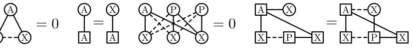
We now give an example of evaluating a decorated constraint. Consider a partitioned graphonW, which is depicted in Figure 1, with partsAandBeach of size 1/2; the graphon

W is equal to 1/2 onA2_{, to 1/3 onA×B, and to 1 on B}2_{. Let H be the decorated graph}

with two adjacent roots both decorated with A and two adjacent non-root vertices v1

and v2 both decorated with B such that v1 is adjacent to only one of the roots and v2 is

adjacent to both roots; the decorated graph H is also depicted in Figure 1. IfH appears in a decorated constraint, then its value is independent of the choice of the roots in the part A and is always equal to 2/81, which is the probability as defined in the previous paragraph.

A

A

B

B A

B

A B

=

Figure 1: An example of evaluating a decorated constraint. The root vertices are depicted by squares and the non-root vertices by circles. The graphon is equal to 1/2 onA2_{, to 1/3}

Note that the condition on them-tuplex1, . . . , xmis equivalent to that there is a positive

probability that a W-random graph with the vertices x1, . . . , xm is H0. Also note that,

unlike in the definition of the density of a graph in a graphon, we do not allow permuting any vertices. For example, ifW is the graphon (with a single part) that is equal top∈[0,1] almost everywhere, then the cherry K1,2 with each vertex decorated with the single part

of W would take the value p2_{(1−p) in a decorated constraint.}

The next lemma, proven in [16], asserts that every decorated constraint is equivalent to a non-decorated constraint.

Lemma 5. Let k ∈ N_{, let a1, . . . , ak be positive real numbers summing to one, and let}

d1, . . . , dk be distinct reals between zero and one. For every decorated constraint C, there

exists a constraint C′ _{such that any partitioned graphon W with parts of sizes a}

1, . . . , ak

and degrees d1, . . . , dk satisfies C if and only if it satisfies C′.

In particular, if a graphonW is a unique partitioned graphon up to weak isomorphism that satisfies a finite collection of decorated constraints, then it is a unique graphon satis-fying a finite collection of ordinary constraints by Lemmas 4 and 5, and hence W is finitely forcible.

We will visualize decorated constraints using the convention from [12], which we now describe and have already used in Figure 1. The root vertices of decorated graphs in a decorated constraint will be depicted by squares and the non-root vertices by circles; each vertex will be labeled with its decoration, i.e., the part that it should be contained in. The roots will be in all the decorated graphs in the constraint in the same mutual position, so it is easy to see the correspondence of the roots of different decorated graphs in the same constraint. A solid line between two vertices represents an edge, and a dashed line represents a non-edge. The absence of a line between two root vertices indicates that the decorated constraint should hold for both the root graph containing this edge and not containing it. Finally, the absence of a line between a non-root vertex and another vertex represents the sum of decorated graphs with this edge present and without this edge. If there arek such lines absent, the figure represents the sum of 2k _{possible decorated graphs}

with these edges present or absent.

We finish this subsection with two auxiliary lemmas. The first is a lemma stated in [12], which essentially states that if a graphon W0 is finitely forcible in its own right, then it

may be forced on a part of a partitioned graphon without altering the structure of the rest of the graphon.

Lemma 6. Letk ∈N_{, m∈[k], leta1, . . . , ak be positive real numbers summing to one, and}

let d1, . . . , dk be distinct reals between zero and one. If W0 is a finitely forcible graphon,

then there exists a finite set C of decorated constraints such that any partitioned graphon W with parts of sizes a1, . . . , ak and degrees d1, . . . , dk satisfies C if and only if there

exist measure preserving maps ϕ0 : [0,1] → [0,1] and ϕm : [0, am] → Am such that

W(ϕm(xam), ϕm(yam)) = W0(ϕ0(x), ϕ0(y)) for almost every (x, y) ∈ [0,1]2, where Am

Note that Lemma 5 implies that the set C of decorated constraints from Lemma 6 can be turned into a set of ordinary (i.e., non-decorated) constraints.

The second lemma is implicit in [24, proof of Lemma 3.3]; its special case has been stated explicitly in, e.g., [12, Lemma 8].

Lemma 7. Let X, Z ⊆ R _{be two measurable non-null sets, and let F :X×Z →[0,1] be}

a measurable function. If there exists C ∈R _{such that}

Z

Z

F(x, z)F(x′, z)dz =C

for almost every (x, x′_)∈X2_{, then}

Z

Z

F(x, z)2 dz =C

for almost every x∈X.

2.2

Regularity partitions and step functions

A step function W : [0,1]2 _{→ [−1,1] is a measurable function such that there exists a}

partition of [0,1] into measurable non-null sets U1, . . . , Uk that W is constant on Ui ×Uj

for every i, j ∈ [k]. A non-negative symmetric step function is a step graphon. If W is a step function (in particular, W can be a step graphon) and A and B two measurable subsets of [0,1], then the density dW(A, B) between A and B is defined to be

dW(A, B) =

Z

A×B

W(x, y) dxdy.

We will omit W in the subscript ifW is clear from the context. Note that it always holds that |d(A, B)| ≤ |A| · |B|. We remark that the definition of dW(A, B) and the definition

of the cut norm given below extend to a wider class of functions from [0,1]2 _{to R, which}

are called kernels; since we will use these definition for step functions, we present them in the setting of step functions only. A step function W′ _{refines a step function W with}

parts U1, . . . , Uk, if each part of W′ is a subset of one of the parts of W and the density

dW(Ui, Uj) between Ui andUj is equal to the weighted average of the densities between the

pairs of those parts of W′ _{that are subsets of U}

i and Uj, respectively.

We next recall the notion of the cut norm. If W is a step function, then the cut norm

of W, denoted by ||W||, is

sup

A,B⊆[0,1]

Z

A×B

W(x, y) dxdy

,

of step functions as the L1-norm; this can be verified following the lines of the analogous

arguments for graphons in [22, Chapter 8]. We emphasize that we do not allow applying a measure preserving transformation to the domain of graphons unlike in the definition of the cut distance. It can be shown [22, Lemma 10.23] that if H is a k-vertex graph andW

and W′ _{are two graphons, then}

|d(H, W)−d(H, W′)| ≤

k

2

||W −W′|| .

Finally, we will say that two graphons W and W′ _{are ε-closeif ||W−W}′_||

≤ε.

A partition of [0,1] into measurable non-null sets U1, . . . , Uk is said to be ε-regular if

d(A, B)− X

i,j∈[k]

d(Ui, Uj)

|Ui||Uj|

|Ui∩A||Uj ∩B|

≤ε

for every two measurable subsets A and B of [0,1]. In other words, the step graphon W′

with parts U1, . . . , Uk that is equal to

d(Ui,Uj)

|Ui||Uj| on Ui×Uj is ε-close to W in the cut norm

metric. In particular, the step graphon W′ _{determines the densities of k-vertex graphs in} W up to an additive error of k₂

ε.

The Weak Regularity Lemma of Frieze and Kannan [14] extends to graphons as follows (see [22, Section 9.2] for further details): for every ε >0, there exists K ≤2O(ε−2), which depends onεonly, such that every graphon has anε-regular partition with at mostK parts. This dependence ofK onεis best possible up to a constant factor in the exponent [11]. We will need a slightly stronger version of this statement, which we formulate as a proposition; its proof is an easy modification of a proof of the standard version of the statement, e.g., the one presented in [22, Section 9.2].

Proposition 8. For every ε > 0 and k ∈ N_{, there exists K ∈} N _{such that for every}

graphon W and every partition U1, . . . , Uk of [0,1] into disjoint measurable non-null sets,

there exist an ε-regular partitionU′

1, . . . , UK′ ′ of [0,1]withK′ ≤K such that every partUi′,

i∈[K′_{], is a subset of one of the parts U}

1, . . . , Uk.

For a step function W, we define d(Γ4, W) to be the following integral:

d(Γ4, W) =

Z

[0,1]4

W(x, y)W(x′, y)W(x, y′)W(x′, y′) dxdx′ dydy′ .

Note that the definition ofd(Γ4, W) coincides with the standard definition oft(C4, W), see

e.g. [22]. In particular, if W is a graphon, then it holds that

d(Γ4, W) =

1

3d(C4, W) + 1 3d(K

−

4 , W) +d(K4, W) ,

it is equal to the expected density of non-induced copies of C4 in a W-random graph.

If W is a step function, then d(Γ4, W) ≤ 4||W||. However, the converse also holds:

d(Γ4, W) ≥ ||W||4; we refer e.g. to [22, Section 8.2], where a proof for symmetric step

functionsW is given and this proof readily extends to the general case. Lemma 11, which we present further, aims at a generalization of this statement to step graphons. Before we can state this lemma, we need to prove two auxiliary lemmas, which we state for matrices rather than step functions for simplicity.

Lemma 9. Let M be aK×K real matrix and let i, j ∈[K]. DefineN to be the following K×K matrix:

Nx,y =

Mi,y+Mj,y

2 if x=i or x=j, and Mx,y otherwise.

It holds that TrMMT_MMT _≥TrNNT_NNT_.

Proof. Set M(x, y), x, y ∈[K], to be the following quantity:

M(x, y) =

K

X

z=1

Mx,zMy,z ,

and define N(x, y),x, y ∈[K], in the analogous way. Observe that

TrMMTMMT −TrNNTNNT =

K

X

x,y=1

M(x, y)2−N(x, y)2 .

We now analyze the difference on the right hand side of the equality by grouping the terms on the right hand side into disjoint sets such that the sum of the terms in each set is non-negative.

The terms with x, y ∈[K]\ {i, j}form singleton sets; note that M(x, y) =N(x, y) for each such term. Fix x ∈ [K]\ {i, j} and consider the two terms corresponding to y = i

and y=j. It follows that

M(x, i)2+M(x, j)2−N(x, i)2−N(x, j)2 =

M(x, i)2+M(x, j)2 −2

K

X

z=1 Mxz

Mi,z+Mj,z

2

!2

=

M(x, i)2 +M(x, j)2− 1

2(M(x, i) +M(x, j))

2

=

1

2M(x, i)

2₊ 1

2M(x, j)

2_{−M(x, i)M(x, j) =} 1

2(M(x, i)−M(x, j))

2

.

Hence, the sum of any pair of such terms is non-negative. The analysis of the terms with

The remaining four terms that have not been analyzed are the terms corresponding to the following pairs (x, y): (i, i), (i, j), (j, i) and (j, j). In this case, we obtain the following:

M(i, i)2+ 2M(i, j)2+M(j, j)2−N(i, i)2 −2N(i, j)2−N(j, j)2 =

M(i, i)2+ 2M(i, j)2+M(j, j)2−4

M(i, i) + 2M(i, j) +M(j, j) 4

2

=

1

4(M(i, i)−M(j, j))

2

+1

2(M(i, i)−M(i, j))

2

+ 1

2(M(j, j)−M(i, j))

2

.

Hence, the sum of these four terms is also non-negative, and the lemma follows.

The next lemma follows by repeatedly applying Lemma 9 to pairs of rows of the matrix

M with indices from the same set Ai and to pairs of rows of the matrix MT with indices

from the same set Bi, and considering the limit matrix N.

Lemma 10. Let M be a K×K real matrix. Further, let X1, . . . , Xk be a partition of [K]

into k disjoint sets and let Y1, . . . , Yℓ be a partition of [K] into ℓ disjoint sets. Define the

K×K matrix N as follows. If x∈Xi, y∈Yj, then

Nx,y =

1

|Xi| · |Yj|

X

x′_∈Xi,y′_∈Yj

Mx′_,y′ .

It holds that TrMMT_MMT _=TrMT_MMT_{M ≥TrNN}T_NNT _=TrNT_NNT_N.

The following auxiliary lemma can be viewed as an extension of [22, Lemma 8.12], which states thatd(Γ4, W)≥ ||W||4 for every graphonW, from the zero graphon to general step

graphons (consider the statement forW0 being the zero graphon). We remark that we have

not tried to obtain the best possible dependence on the parameter ε in the statement of the lemma. The lemma also holds in a more general setting, where the parts of graphons are not required to be of the same size.

Lemma 11. Let W0 be a step graphon with all parts of the same size, and W a step

graphon refining W0 such that all parts of W have the same size. If ||W−W0|| ≥ε, then

d(Γ4, W)≥d(Γ4, W0) +ε4/8.

Proof. Since ||W −W0|| ≥ ε, there exist two measurable subsets A and B of [0,1] such

that

Z

A×B

W(x, y)−W0(x, y) dxdy

≥ε. (1)

Let U be one of the parts of the graphon W. Depending whether R

U×BW −W0 dx dy is

positive or negative, replacingA with either A∪U orA\U does not decrease the integral in (1). Hence, we can assume that each part ofW is either a subset ofA or is disjoint from

A, and the same holds with respect to B (but different parts U of W may be contained in

Let k be the number of parts of W0 and K the number of parts W. Further, let M

be the K ×K matrix such that the entry Mi,j, i, j ∈K, is the density of W between its

i-th and the j-th parts, and let P be the K ×K matrix such that Pi,j, i, j ∈ K, is the

density ofW0between thei-th and thej-th parts ofW. LetUi,i∈[k], be the subset of [K]

containing the indices of the parts ofW contained in thei-th part ofW0. Observe that both

matrices M andP are symmetric and the matrixP is constant on each submatrix indexed by pairs from Ui×Uj for some i, j ∈[k]. Since d(Γ4, W) = TrM4 and d(Γ4, W0) = Tr P4,

our goal is to show that Tr M4_{−Tr P}4 _{≥ ε}4_{/8. Finally, let A}′ _{be the indices of parts of} W contained in A, and let B′ _{be the indices of parts of W contained in B. Observe that}

(1) yields that the sum of the entries of the matrix M −P with the indices in A′ _×B′ _is

either at least ε or at most −ε.

Let N be the matrix from the statement of Lemma 10 for the matrix M, Xi = {i},

i∈[K], and Yj =Uj, j ∈[k]. Let ε1 be the sum of the entries of the matrix M −N with

the indices in A′ _×B′_{, and let ε}

2 be the sum of the entries of the matrix N −P with the

indices in A′_×B′_{. Note that |ε}

1+ε2| ≥ ε, which implies that |ε1|+|ε2| is at least ε. By

Lemma 10, it holds that Tr M4 _−TrNNT_NNT _{≥0. Since P}T _{can be obtained from the}

matrix NT _{by applying Lemma 10 with X}

i ={i}, i∈[K], and Yj =Uj,j ∈[k], it follows

that TrNT_NNT_{N −TrP}4 _{= TrNN}T_NNT _−TrP4 _≥0.

We now show that Tr M4 _{−Tr NN}T_NNT _{≥ ε}4

1. Let Q = M −N. We now want to

analyze the entries of the matrix (N +αQ)(N +αQ)T _{for α ∈ [0,1]. Fix x, y ∈ [K] and}

observe that the entry in thex-th row and they-th column of the matrix (N+αQ)(N+αQ)T

is equal to

k

X

j=1

X

z∈Uj

(N +αQ)x,z(N +αQ)y,z .

The definition of the matrixN implies that

X

z∈Uj

Qx,z=

X

z∈Uj

Qy,z = 0

for everyj ∈[k]. It also holds that Nx,z =Nx,z′ andN_y,z =N_y,z′ for any z and z′ from the

same set Uj, j ∈ [k], which implies that the entry of the matrix (N +αQ)(N +αQ)T in

the x-th row and the y-th column is

K

X

z=1

Nx,zNy,z +α2Qx,zQy,z .

Hence, we conclude that (N +αQ)(N +αQ)T _=NNT _+α2_QQT_{. It follows that}

Tr (N+αQ)(N +αQ)T_{(N +αQ)(N +αQ)}T ₌

TrNNT_NNT _{+ 2α}2_{Tr NN}T_QQT _+α4_TrQQT_QQT _{. (2)}

By Lemma 10 applied with M =N +αQ and the same sets Xi and Yj as earlier,

for every α ≥ 0, which implies that Tr NNT_QQT _{≥ 0. In particular, we obtain from (2)}

for α= 1 that

TrM4−TrNNT_NNT ₌

Tr (N +αQ)(N+αQ)T_{(N +αQ)(N +αQ)}T _−TrNNT_NNT _≥

TrQQT_QQT _{. (3)}

Since the cut-norm of the step graphon corresponding to Q is at least ε1, it follows that

TrQQT_QQT _≥ε4 1.

Applying the symmetric argument to the matrices PT _{and N}T _{=N, we obtain that}

TrNNT_NNT _−TrP4 _{≥Tr (N −P)(N −P)}T_{(N −P)(N−P)}T _≥ε4

2 . (4)

Since TrM4_−TrNNT_NNT _{≥0 and TrN}T_NNT_{N −TrP}4 _{≥0, we obtain from (3) and}

(4) using |ε1|+|ε2| ≥ε that Tr M4−TrP4 ≥ε41 +ε42 ≥ε4/8, as desired.

3

General setting of the proof of Theorem 1

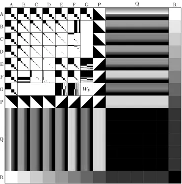
In this section, we provide a general overview of the structure of the graphon W0 from

Theorem 1 and the proof of Theorem 1. The visualization of the structure of the graphon

W0 can be found in Figure 2. The proof of Theorem 1 is spread through Sections 3–6, with

this section containing its initial steps.

Fix a graphon WF. The graphon W0 is a partitioned graphon with 10 parts denoted

by capital letters from A to R. Each part except for Q has size 1/14, and the size of Q

is 5/14. If X, Y ∈ {A, . . . , G, P, Q, R} are two parts, the restriction of the graphonW0 to X ×Y will be referred to as the tile X ×Y. The graphon WF will be contained in the

tile G×G of the graphon W0. The degrees of the parts (i.e., the degrees of the vertices

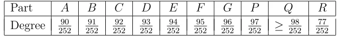
forming the parts) are given in Table 1; the degree ofQis at least 5/14 + 8/252, i.e., larger than the degree of any other part, and will be fixed later in the proof.

Part A B C D E F G P Q R

Degree ₂₅₂90 ₂₅₂91 ₂₅₂92 ₂₅₂93 ₂₅₂94 ₂₅₂95 ₂₅₂96 ₂₅₂97 ≥ ₂₅₂98 ₂₅₂77

Table 1: The degrees of the vertices in the parts of the graphon W0 from the proof of

Theorem 1.

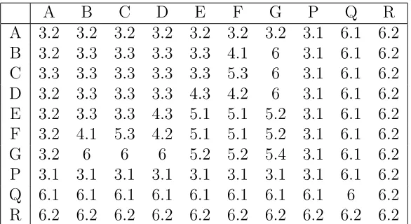
Rather than giving a complex definition of the graphon W0 at once, we decided to

present the particular details of the structure ofW0 together with the decorated constraints

fixing the structure of W0 in Sections 3–6. Table 2 gives references to subsections where

the individual tiles of the graphon W0 are considered and the corresponding decorated

constraints are given.

We now start the proof of the finite forcibility of the graphonW0. LetW be a graphon

A B C D E F G P Q R

A

B

C

D

E

F

G

P

Q

R

WF

A B C D E F G P Q R A 3.2 3.2 3.2 3.2 3.2 3.2 3.2 3.1 6.1 6.2 B 3.2 3.3 3.3 3.3 3.3 4.1 6 3.1 6.1 6.2 C 3.3 3.3 3.3 3.3 3.3 5.3 6 3.1 6.1 6.2 D 3.2 3.3 3.3 3.3 4.3 4.2 6 3.1 6.1 6.2 E 3.2 3.3 3.3 4.3 5.1 5.1 5.2 3.1 6.1 6.2 F 3.2 4.1 5.3 4.2 5.1 5.1 5.2 3.1 6.1 6.2 G 3.2 6 6 6 5.2 5.2 5.4 3.1 6.1 6.2 P 3.1 3.1 3.1 3.1 3.1 3.1 3.1 3.1 6.1 6.2 Q 6.1 6.1 6.1 6.1 6.1 6.1 6.1 6.1 6 6.2 R 6.2 6.2 6.2 6.2 6.2 6.2 6.2 6.2 6.2 6.2

Table 2: Subsections where the structure of the tiles are presented and the related decorated constraints then given.

parts of W0 and that satisfies all the decorated constraints given in Sections 3–6. It will

be obvious that the graphon W0 also satisfies these constraints. So, if we show that W is

weakly isomorphic to W0, then we will have established that W0 is finitely forcible. We

will achieve this goal by constructing a measure preserving mapg : [0,1]→[0,1] such that

W(x, y) =W0(g(x), g(y)) for almost every (x, y)∈[0,1]2.

Let A, . . . , G, P, Q, R be the parts of the graphon W. To make a clear distinction between the parts of W and W0, we will use A0, . . . , G0, P0, Q0, R0 ⊆ [0,1] to denote the

subintervals forming the parts ofW0. The Monotone Reordering Theorem [22, Proposition

A.19] implies that, for every X ∈ {A, . . . , G, P, Q, R}, there exist a measure preserving map ϕX :X→[0,|X|) and a non-decreasing function ˜fX : [0,|X|)→R such that

˜

fX(ϕX(x)) = degPW(x) =

1

|P|

Z

P

W(x, y) dy

for almost every x∈X. The function g maps the vertex x∈X, X∈ {A, . . . , G, P, Q, R}, of W to the vertex ηX(ϕX(x)/|X|) where ηX is the bijective linear map from [0,1) to the

part X0 of the graphon W0 of the form ηX(x) = |X0| ·x+cX for some cX ∈ [0,1] (we

intentionally define ηX in this way, instead of defining ηX as a linear measure preserving

map from [0,|X0|) to X0, since this definition simplifies our exposition later). In addition,

we define a function fX : X → [0,1] as fX(x) = ˜fX(ϕX(x)) for every x ∈ X. Clearly,

g is a measure preserving map from [0,1] to [0,1]; hence, we “only” need to show that

W(x, y) =W0(g(x), g(y)) for almost every (x, y)∈[0,1]2.

3.1

Coordinate system

In this subsection, we analyze the tile P ×P and the tilesP ×X (and the symmetric tiles

equal to 1 ifx+y≥1 and equal to 0 otherwise; the half-graphon is finitely forcible as shown in [13, 24]. Consider the decorated constraints from Lemma 6 forcing the tile P ×P to be weakly isomorphic to the half-graphon. This implies that ˜fP(x) =ϕP(x)/|P| for every

x ∈ [0,|P|), where ϕP and ˜fP are the functions from the Monotone Reordering Theorem

used to define the function g. Lemma 6 and the finite forcibility of the half-graphon yield that W(x, y) =W0(g(x), g(y)) for almost every (x, y)∈P2.

P X

P X

= 0

P Y

P P

=

P Z

= 1

−

Figure 3: Decorated constraints forcing the tiles X × P where X ∈ {A, . . . , G}, Y ∈ {E, F, G}and Z ∈ {A, B, C, D}.

Next consider the decorated constraints depicted in Figure 3 and fix X ∈ {A, . . . , G}. The first constraint in Figure 3 implies thatW(x, y)∈ {0,1}for almost every (x, y)∈P×X

and that NX

W(x) ⊑ NWX(x′) or NWX(x′) ⊑ NWX(x) for almost every pair (x, x′) ∈ P2. In

addition, the choice of the function ϕX implies that almost every pair y, y′ ∈ X satisfies

the following: if ϕX(y) ≤ ϕX(y′), then degPW(y) ≤ deg P

W(y′). Hence, the first constraint

and the choice of ϕX yield that for almost every x∈ P, there exists t ∈[0,|X|] such that

the set NX

W(x) and ϕ

−1

X ([0, t)) differ on a null set. We conclude that there exists a function

hX :P →[0,1] such that it holds for almost every (x, y)∈P ×X thatW(x, y) = 1 if and

only if ϕX(y)/|X| ≥ 1−hX(x).

If X ∈ {E, F, G}, then the second constraint in Figure 3 implies that degX_{(x) =}

|NX_{(x)| = deg}P

(x) for almost every x ∈ P, i.e., hX(x) = fP(x). Since it holds that

W(x, y) = 1 if and only if ϕX(y)/|X| ≥ 1−hX(x) for almost every (x, y) ∈ P ×X, we

obtain that ˜fX(y) = ϕX(y)/|X| for y ∈ [0,|X|), W(x, y) = 1 for almost every (x, y) ∈

P ×X with fP(x) +fX(y) ≥ 1 and W(x, y) = 0 for almost every (x, y) ∈ P ×X with

fP(x)+fX(y)<1. It follows thatW(x, y) =W0(g(x), g(y)) for almost every (x, y)∈P×X,

where X ∈ {E, F, G}. The analogous argument using the third constraint in Figure 3 implies that degX(x) = |NX_{(x)| = |X| −deg}P

(x) for almost every x ∈ P, which yields that W(x, y) =W0(g(x), g(y)) for almost every (x, y)∈P ×X, where X ∈ {A, B, C, D}.

We conclude this subsection by observing that degP_W(x) = fX(x) for almost every

x∈ X, where X ∈ {A, . . . , G} ∪ {P}. In particular, we may interpret the relative degree of a vertex with respect to P as its coordinate. Also observe that NP

W(x) ⊑ NWP(x′) for

almost every pair (x, x′_{)∈X×X such that f}

X(x)≤fX(x′).

3.2

Checker tiles

for k ∈ N_{0 and set WC(x, y) equal to 1 if (x, y)∈}

∞

S

k=0 I2

k, i.e., both x and y belong to the

same Ik, and equal to 0 otherwise. The checker graphon WC is depicted in Figure 4. We

remark that we present an iterated version of this definition in Subsection 3.3. We set

W0(ηA(x), ηX(y)) =WC(x, y) for x, y ∈[0,1)2 whereX ∈ {A, . . . G}.

Figure 4: The checker graphonWC.

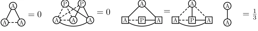
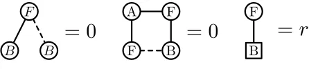
Consider the decorated constraints in Figure 5, which we claim to force the structure of the tile A×A. The argument follows the lines of the analogous argument given in [16, Section 5], so we sketch the main steps here and refer the reader for full details to [16]. The first constraint in Figure 5 implies that there exists a collection JA of disjoint measurable

non-null subsets of A such that the following holds for almost every (x, y) ∈ A × A:

W(x, y) = 1 if and only if x and y belong to the same set J ∈ JA, and W(x, y) = 0

otherwise.

A A

A

= 0

A A A

P P

= 0

A P A A P A

A A

=

A A

=

Figure 5: The decorated constraints forcing the structure of the tile A×A.

The second constraint in Figure 5 implies that almost every triple (x, x′_{, x}′′_{) ∈ A}3

satisfies that if x and x′′ belong to the same set J ∈ JA and fA(x) < fA(x′) < fA(x′′),

then x′ _{also belongs to the set J (since x and x}′ _{cannot be non-adjacent). This implies}

that for every J ∈ JA, there exists an open interval J′ such that J and f_A−1(J′) differ on

a null set. Let J′

A be the collection of these open intervals for different sets J ∈ JA; since

fA is a measure preserving map and the sets in JA are disjoint, the intervals in JA′ must

be disjoint.

The third constraint in Figure 5 implies that almost every pair (x, x′_)∈A2 _{satisfies that}

ifxandx′ _{belong to the same setJ ∈ J}

AandfA(x)< fA(x′), then|NWA(x)∩NWA(x′)|=|J|

is the measure of the set Y of the points y ∈ A such that y 6∈ J and fA(y) > fP(x′′) for

almost every x′′ _{∈ P with f}

A(x) < fP(x′′) < fA(x′). Observe that if J is fixed and

J = f_A−1(J′_{) for J}′ _{∈ J}′

A, then the set Y differs from f

−1

A ([supJ′,1)) on a null set. It

follows that the measure |J| =|J′_{| is equal to 1−supJ}′_{. Hence, each interval in J}′

the form (1−2γ,1−γ) for some γ ∈(0,1/2]; let Γ be the set of all the values of γ for that there is a corresponding interval in J′

A. Note that if γ ∈ Γ, then Γ∩(γ/2, γ) = ∅, which

implies in particular that the set Γ is countable. Let γk be thek-th largest value in the set

Γ and in case that Γ is finite, set γk = 0 for k > |Γ|. It follows that

1

|A|2

Z

A×A

W(x, y) dxdy= X

J′_∈J′

A

(supJ′−infJ′)2 =X

k∈N

γk2 .

The last constraint in Figure 5 implies that the integral on the left hand side of the above equality is equal to 1/3, which is possible only ifγk = 2−k for every k∈N. It follows that

W(x, y) =W0(g(x), g(y)) for almost every (x, y)∈A2.

A X

A

= 0

A X

=

X X X

A P P

= 0

X P X X P X

X X

A A

=

Figure 6: The decorated constraints forcing the structure of the tiles A×X where X ∈ {B, . . . , G}.

We now consider the decorated constraints from Figure 6. Fix X ∈ {B, . . . , G}. The first constraint in Figure 6 implies that for every J ∈ JA, there exists a measurable set

Z(J)⊆X such that the following holds for almost every pair (x, y)∈A×X: W(x, y) = 1 if x ∈ J and y ∈ Z(J), and W(x, y) = 0 otherwise. Note that the sets Z(J) need not be disjoint. The second constraint in Figure 6 yields that degAW(x) = deg

X

W(x) for

almost every x∈A, which implies that the sets J and Z(J) have the same measure. The third constraint implies that the following holds for almost every triple (y, y′_{, y}′′_{) ∈ X}3_:

if fP(y) < fP(y′) < fP(y′′), y ∈ Z(J) and y′′ ∈ Z(J), then y′ ∈ Z(J). Consequently,

for every Z(J), there exists an open interval Z′_{(J) such that Z(J) differs from the set} g_X−1(Z′_{(J)) on a null set. Finally, the last constraint in Figure 6 yields that the following}

holds for almost every x ∈ J: the measure of NX

W(x) = Z(J), which is |Z(J)| = |Z′(J)|,

is equal to the measure of the set containing all y 6∈ Z(J) with fX(y) ≥ supZ′(J). It

follows that the interval Z′_{(J) is equal to (1−2γ, γ) for some γ ∈ (0,|X|/2]. Since the}

measures of J and Z′_{(J) are the same, it must hold that Z}′_{(J) = J}′ _{where J}′ _{∈ J}′

A is

the interval corresponding to J. It follows that W(x, y) =W0(g(x), g(y)) for almost every

(x, y)∈A×X.

3.3

Iterated checker tiles

The checker graphon WC represents a large graph formed by disjoint complete graphs on

the 1/2,1/4,1/8, . . .fractions of its vertices. We now present a family of iterated checker graphons. Informally speaking, we start with the checker graphonWC and at each iteration,

Figure 7: The iterated checker graphons W0

C, WC1 and WC2.

is as follows. Fix k ∈N_{0. If k = 0, define Ij}

0,j0 ∈N0, to be the interval

Ij0 =

1−2−j0_,1−2−j0−1_.

If k >0, we define Ij0,...,jk for (j0, . . . , jk)∈N

k

0 as Ij0,...,jk =

supIj0,...,jk−1 −2

−jk_|I

j0,...,jk−1|,supIj0,...,jk−1 −2

−jk−1_|I

j0,...,jk−1|

.

The k-iterated checker graphon Wk

C is then defined as follows: WCk(x, y) is equal to 1 if

there exists a (k+ 1)-tuple (j0, . . . , jk)∈Nk0 such that both xand y belong to the interval Ij0,...,jk, and it is equal to 0 otherwise. The iterated checker graphonsW

0

C,WC1 and WC2 are

depicted in Figure 7. Note that W0

C = WC and the definition of Ij0 coincides with that

given in Subsection 3.2. We will also refer to an interval Ij0,...,jk as to a k-iterated binary

interval.

For X ∈ {B, C} and Y ∈ {X, . . . , E}, we set

W0(ηX(x), ηY(y)) =

W1

C(x, y) if X =B, and

W2

C(x, y) if X =C

for all x, y ∈[0,1)2_{. We also set the tile D×D to be such that}

W0(ηD(x), ηD(y)) =WC3(x, y)

for all x, y ∈ [0,1)2_{. This also defines the values of W}

0 in the symmetric tiles, i.e., the

values for the tile X×Y determine the values for the tile Y ×X.

Consider the decorated constraints depicted in Figures 8 and 9. We first analyze the structure of the tileB×B, then all the tiles B×Y, Y ∈ {B, . . . , E}, then the tile C×C, then all the tiles C×Y,Y ∈ {C, . . . , E}, before finishing with the tile D×D. Fix (X, Y) to be one of the pairs (A, B),(B, C) or (C, D). We assume that W(x, y) = W0(g(x), g(y))

for almost every (x, y)∈X×X and almost every (x, y)∈X×Y, and our goal is to show that W(x, y) =W0(g(x), g(y)) for almost every (x, y)∈Y ×Y.

The first two constraints on the first line in Figure 8 imply that there exists a collection

J′

Y of disjoint open intervals such that the following holds for almost every (x, y) ∈ Y2:

W(x, y) is equal to 1 if and only if fY(x) and fY(y) belong to the same interval J′ ∈ JY′,

and it is equal to 0 otherwise. The third constraint on the first line in Figure 8 yields that each interval inJ′

Y Y Y

= 0

Y Y Y

P P

= 0

X Y

Y

= 0

Y P Y Y P Y

Y Y

X X

=

X X

Y Y

X X

=

Figure 8: The decorated constraints forcing the structure of the tiles B2_{, C}2_{, and D}2_,

where (X, Y)∈ {(A, B),(B, C),(C, D)}.

X

Z Y

X

= 0

Z Z Z

Y P P

= 0

Y Y

=

Z Z

Z Z

Z P Z P

Y Y

X X

=

Figure 9: The decorated constraints forcing the structure of the iterated checker graphons on the non-diagonal tiles, where (X, Y)∈ {(A, B),(B, C)}andZ ∈ {C, D, E, F}if X =A

The first constraint on the second line in Figure 8 yields that the following holds for almost every triple (x, y, y′_{) ∈ X×Y ×Y such that f}

Y(y) and fY(y′) are from the same

interval J′

Y ∈ JY′ and fX(x) is from the interval JX′ ∈ JX′ that is a superinterval of JY′ :

the measure ofJ′

Y (which is equal to the left hand side of the equality) is the same as the

measure of the set of all y′′ _{such thatf}

Y(y′′)∈JX′ and fY(y′′)>supJY′ (which is equal to

the right hand side). It follows that

JY′ = (supJX′ −2γ,supJX′ −γ)

for some γ ∈ (0,|J′

X|/2]. The very last constraint in Figure 8 yields for every JX′ ∈ JX′

that

X

J′

Y∈JY′,JY′⊆JX′

|J_Y′ |2 = 1 3|J

′

X|

2_.

However, this is only possible if the set J′

Y contains all intervals of the form (supJX′ −

2γ,supJX′ −γ) for every JX′ ∈ JX′ and every γ = |JX′ | ·2−i, i ∈ N. It follows that

W(x, y) =W0(g(x), g(y)) for almost every (x, y)∈Y ×Y.

We continue to fix a pair (X, Y) ∈ {(A, B),(B, C)}, but in addition we now fix

Z ∈ {Y, . . . , E} \ {Y} where Y ∈ {B, C}. Our next goal is to show that W(y, z) =

W0(g(y), g(z)) for almost every (y, z)∈Y ×Z, which is achieved using the decorated

con-strains given in Figure 9. The first constraint in Figure 9 implies that it holds for almost every y ∈ Y that fZ(NWZ(y)) ⊑ JX′ where JX′ is the unique interval of JX′ containing

fY(y). The second constraint in Figure 9 yields that for almost every y ∈Y, there exists

an interval Jy such that NWZ(y) and fZ−1(Jy) differ on a null set, W(y, z) = 1 for almost

every z ∈fZ−1(Jy), and W(y, z) = 0 for almost everyz ∈Z\fZ−1(Jy). The third constraint

yields that degY_W(y) = degZ_W(y) for almost every y∈Y, i.e., the measure of Jy is the same

as the measure of the interval in JY containing fY(y).

Finally, the last constraint in Figure 9 implies that almost every quadruple x ∈ X,

y∈Y,z, z′ _{∈Z such thatf}

Z(z)< fZ(z′),fZ(z) andfZ(z′) belong to the intervalJy, which

is a subinterval ofJ′

X ∈ JX′ withfX(x)∈JX′ , satisfies that the measure ofNWZ(y) (note that

NZ

W(y) is a subset offZ−1(JX′ )) and the measure of allz′ ∈fZ−1(JX′ )\NWZ(y) with fZ(z′)>

supJy are equal. In particular, the interval Jy is of the form (supJX′ −2γ,supJX′ −γ)

for almost every y ∈ Y, where J′

X is the unique interval of JX′ containing fY(y). Hence,

the interval Jy is equal to the interval in JY′ containing fY(y) for almost every y ∈Y. It

follows that W(y, z) =W0(g(y), g(z)) for almost every (y, z)∈Y ×Z.

4

Encoding the target graphon

In this section, we describe how the densities in dyadic squares of the graphon WF are

wired in a single binary sequence, which will be encoded in the tileB×F. To achieve this, we need to fix a mapping ϕ fromN4

0 to N0. Let us define this mapping as follows. The

4-tuples (a, b, c, d) with the same sums=a+b+c+dof their entries are injectively mapped to the numbers between s+3₄

and s+4₄

− 1 in the lexicographic order. For example,

4.1

Encoding dyadic square densities

The tile B ×F encodes the edge densities on all dyadic squares of WF. Let Id(s) be the

interval _s

2d, s+1

2d

, and define ford, s, t∈N_{0 the valueδ(d, s, t) as}

δ(d, s, t) = 22d_·

Z

Id_(s)×Id_(t)

WF(x, y) dxdy

if 0 ≤ s, t ≤ 2d _{−1, and δ(d, s, t) = 0, otherwise. If W}

F is the one graphon, i.e., WF is

equal to 1 almost everywhere, we fix r = 1. Otherwise, we fix r ∈ [0,1) to be the unique real satisfying that

δ(d, s, t) =

∞

X

p=0

2−p_r

ϕ(d,s,t,p)+1 , and (5)

that for alld, s, t∈N_{0, the value of rϕ(d,s,t,p)+1 is equal to zero for infinitely many p∈}N_0,

where rk is the k-th bit in the standard binary representation of r (with the first bit

following immediately the decimal point). The standard binary representation is the unique representation with infinitely many digits equal to zero If WF is the one graphon, we set

rk = 1 for every k ∈N. Observe thatr is not a multiple of an inverse power of two unless

WF is the zero graphon or the one graphon (r ∈ {0,1} in these two cases).

B B F

= 0

A F

B

= 0

B F

=

r

Figure 10: The decorated constraints forcing the structure of the tile B ×F.

We now define W0(ηB(x), ηF(y)) = rk+1 for x∈[0,1] andy ∈Ik, k∈N0, and force the

corresponding structure of the tileB ×F. Consider the decorated constraints depicted in Figure 10. The first constraint implies that degBW(x)∈ {0,1} for almost every x ∈ F. In

particular,W is{0,1}-valued almost everywhere onB×F. The second constraint implies that for every k∈N_{0 and for almost everyx, x}′ _{∈ f}−1

F (Ik), degBW(x) = deg B

W(x′). Let r′k be

the common degree degBW(x) of the vertices x∈ fF−1(Ik−1), k ∈ N. The last constraint in

the figure implies that

X

k∈N

2−k_r k=

X

k∈N

2−k_r′

k .

Since r is not a non-zero multiple of an inverse power of two unless r ∈ {0,1}, it follows that rk =r′k for allk ∈N. If r ∈ {0,1}, it follows that rk =rk′ =r trivially. We conclude

that W(x, y) =W0(g(x), g(y)) for almost every (x, y)∈B ×F.

4.2

Matching tile

1 if x∈Ia,b,c,d and y∈Iϕ(a,b,c,d) for some (a, b, c, d)∈N40 and to be equal to 0, otherwise.

D

F A

F

= 0

A

F D

F

= 0

F D

D

= 0

D D

F

= 0

F D

=

∞

P

a,b,c,d=0

2

·

2

D

F C

=

P

a,b,c,d=0

2

_·

₂

_·

₂

D

F B

=

P

a,b,c,d=0

2

·

2

·

2

D

F A

=

P

a,b,c,d=0

2

_·

₂

_·

₂

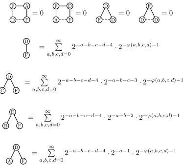
Figure 11: The decorated constraints forcing the structure of the tile D×F.

Consider the decorated constraints in Figure 11. The first constraint implies thatW is

{0,1}-valued almost everywhere in D×F and that for almost every x∈D, it holds that

NF

W(x) =∪k∈Kxf_F−1(Ik) up to a null set for some Kx ⊆N0. The second constraint implies

that for almost every vertex of D, the set Kx has cardinality 0 or 1. The third constraint

yields that for every (a, b, c, d) ∈ N4

0, the set Kx is the same for almost all x ∈ D with

fD(x)∈Ia,b,c,d. Finally, the last constraint in the first line implies that the sets Kx andKy

are disjoint for almost all x, y ∈ D with fD(x) and fD(y) from different 3-iterated binary

intervals.

Let τ(a, b, c, d) be the common degree degFW(x) of vertices x ∈ fD−1(Ia,b,c,d). If Kx is

empty for almost all x∈f_D−1(Ia,b,c,d), then τ(a, b, c, d) = 0; otherwise, τ(a, b, c, d) is 2−k−1,

where k is the unique integer contained in Kx for almost all x ∈ fD−1(Ia,b,c,d). Note that

the non-zero values ofτ(a, b, c, d) are distinct for distinct (a, b, c, d)∈N4

edge density in the tile D×F is the following:

Z

D×F

W(x, y) dxdy= X

(a,b,c,d)∈N4

0

|Ia,b,c,d|τ(a, b, c, d) =

X

s∈N₀

2−(s+4) X

(a,b,c,d)∈N4

0

a+b+c+d=s

τ(a, b, c, d).

The constraint in the second line in Figure 11 yields the following:

X

s∈N₀

2−(s+4) X

(a,b,c,d)∈N4 0

a+b+c+d=s

τ(a, b, c, d) = X

s∈N₀

2−(s+4) X

(a,b,c,d)∈N4 0

a+b+c+d=s

2−ϕ(a,b,c,d)−1 _.

Since the non-zero values of τ(a, b, c, d) are mutually distinct, this equality can hold only if

{τ(a, b, c, d) s.t. a+b+c+d=s}={2−ϕ(a,b,c,d)−1 s.t. a+b+c+d=s}

for every s∈N_0.

The constraint in the third line in Figure 11 implies that

X

(a,b,c,d)∈N4

0

2−a−b−c−d−4·2−a−b−c−3·τ(a, b, c, d) = X

(a,b,c,d)∈N4

0

2−a−b−c−d−4·2−a−b−c−3·2−ϕ(a,b,c,d)−1 .

Since it holds for every s∈N_{0 that}

{τ(a, b, c, d) s.t. a+b+c+d=s}={2−ϕ(a,b,c,d)−1 s.t. a+b+c+d=s},

we get that the following holds for all d∈N_{0 and s∈}N_0:

{τ(a, b, c, d) s.t. a+b+c=s}={2−ϕ(a,b,c,d)−1 s.t. a+b+c=s}.

Similarly, the constraint in the fourth line implies that

X

(a,b,c,d)∈N4 0

2−a−b−c−d−4_·2−a−b−2_{·τ(a, b, c, d) =} X

(a,b,c,d)∈N4 0

2−a−b−c−d−4_·2−a−b−2_·2−ϕ(a,b,c,d)−1 _,

which yields that it holds for allc, d, s∈N_{0 that}

{τ(a, b, c, d) s.t. a+b=s}={2−ϕ(a,b,c,d)−1 s.t. a+b =s}.

Finally, the constraint in the fifth line implies that

X

(a,b,c,d)∈N4 0

2−a−b−c−d−4_·2−a−1_{·τ(a, b, c, d) =} X

(a,b,c,d)∈N4 0

2−a−b−c−d−4_·2−a−1_·2−ϕ(a,b,c,d)−1 _,

which implies thatτ(a, b, c, d) = 2−ϕ(a,b,c,d)−1_{for alla, b, c, d∈N}

D

E

δ(0,0,0)

δ(0,1,0)

δ(1,0,0)

Figure 12: An example of the D×E tile.

4.3

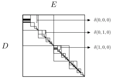
Collating dyadic square densities

The tile D×E is designed to group the values of δ(d, s, t). We set W0(ηD(x), ηE(y)) =

rϕ(d,s,t,p)+1 for allx ∈Id,s,t,p, y ∈Id,s,t and (d, s, t, p)∈N40, and we set W0(ηD(x), ηE(y)) to

be zero elsewhere. An example of a tile with this structure is depicted in Figure 12. Note that the density of the square ηD(Id,s,t)×ηE(Id,s,t) is equal to δ(d, s, t).

Consider the decorated constraints depicted in the Figure 13. The first constraint implies that W(x, y) = 0 for almost every (x, y) such that x∈ fD−1(Id,s,t), y∈ fE−1(Id′_,s′_,t′)

and (d, s, t) 6= (d′_{, s}′_{, t}′_{). The second constraint yields that for almost every x ∈ D such}

that x ∈ f_D−1(Id,s,t), degEW(x) is either 0 or 2−d−s−t−3. In particular, W(x, y) ∈ {0,1} for

almost every (x, y)∈D×E.

D C

E

= 0

E

C E

D

= 0

D C

F B

=

F

Figure 13: The decorated constraints forcing the structure of the tile D×E.

We now analyze the last decorated constraint depicted in the Figure 13. This constraint implies that the following holds for almost every choice of aD-rootxand anF-rootysuch that fD(x)∈Id,s,t,p and fF(y)∈Iϕ(d,s,t,p):

2−d−s−t−3 _·r

ϕ(d,s,t,p)+1= degEW(x) .

It follows that W(x, y) =W0(g(x), g(y)) for almost every (x, y)∈D×E.

5

Forcing the target graphon

In this section, we force the densities in each dyadic square of the tileG×Gto be as in the graphon WF and we argue that the graphon inside the tile is the graphonWF. To achieve

5.1

Dyadic square indices

We start with the tiles E×E, E×F and F ×F, which represent splitting the 0-iterated binary interval Ik into 2k and 22k equal length parts. Formally,W0(ηE(x), ηE(y)) is equal

to 1 for x, y ∈[0,1) if x and y belong to the same 0-iterated binary interval Ik and

x−minIk

|Ik|

·2k

=

y−minIk

|Ik|

·2k

,

and it is equal to 0 otherwise. Similarly, W0(ηF(x), ηF(y)) is equal to 1 forx, y ∈ [0,1) if

x and y belong to the same 0-iterated binary interval Ik and

x−minIk

|Ik|

·22k

=

y−minIk

|Ik|

·22k

,

and it is equal to 0 otherwise. An illustration can be found in Figure 14. Finally, we set

W0(ηE(x), ηF(y)) =W0(ηE(x), ηE(y)) for allx, y ∈[0,1).

Figure 14: Representation of the tiles E×E and F ×F.

X X

X

= 0

X X X

P P

= 0

X A

X

= 0

E E

= 2

A A

F F

= 4

A A

Figure 15: The decorated constraints forcing the tilesE×E andF×F, whereX ∈ {E, F}.

Fix X ∈ {E, F} and consider the decorated constraints given in Figure 15. The three constraints on the first line in Figure 15 imply thatW(x, y)∈ {0,1} for almost every pair (x, y)∈X ×X and that there exists a collection of disjoint open intervalsJX, which are

and fX(y) belong to the same interval J ∈ JX (except for a subset of X×X of measure

zero).

If X = E, then the first constraint on the second line in Figure 15 implies that degWE (x) = 2−2k−1 for almost every x ∈ fE−1(Jk), i.e., if J ∈ JE and J ⊆ Ik, then

|J|= 2−k_|I

k|. Hence, the set JE is formed precisely by the intervals

minIk+

ℓ−1

2k |Ik|,minIk+

ℓ

2k|Ik|

for k∈N_{0 and ℓ∈[2}k_{]. Hence,W(x, y) = W0(g(x), g(y)) for almost every (x, y)∈E×E.}

The analogous argument using the last constraint on the second line in Figure 15 gives that JF is formed precisely by the intervals

minIk+

ℓ−1

22k |Ik|,minIk+

ℓ

22k|Ik|

for k ∈N_{0 and ℓ ∈ [2}2k_{], which leads to the conclusion that W(x, y) = W}

0(g(x), g(y)) for

almost every (x, y)∈F ×F.

F E

E

= 0

F F F

E P P

= 0

E E

F

= 0

E F

=

E P E

F P F

= 0

Figure 16: The decorated constraints forcing the structure of the tile E×F.

It remains to analyze the tile E ×F. Consider the decorated constraints given in Figure 16. The first two constraints in Figure 16 imply that for every J ∈ JE, there exists

an open interval K(J) such that the following holds for almost every (x, y) ∈ E × F:

W(x, y) = 1 if fE(x)∈J and fF(y)∈K(J) for someJ ∈ JE, andW(x, y) = 0 otherwise.

The third constraint implies that the intervals K(J) and K(J′_{) are disjoint for J 6= J}′_,

and the fourth constraint yields that the measure ofK(J) is equal to|J|. Finally, the last constraint implies that if an interval J1 ∈ JE precedes an interval J2 ∈ JE, then K(J1)

precedes the intervalK(J2). We conclude thatK(J) =J for everyJ ∈ JE. Consequently,

W(x, y) =W0(g(x), g(y)) for almost every (x, y)∈E×F.

5.2

Referencing dyadic squares

We now describe the tiles E ×G and F ×G, which allow referencing particular dyadic squares by the intervals from JE and JF. Formally, W0(ηE(x), ηG(y)) = 1 for x, y ∈[0,1)

if and only if x∈Ik and

x−minIk

|Ik|

·2k

=

y·2k