Importance sampling simulation for evaluating lower bound symbol error rate of the Bayesian DFE with multi level signalling schemes

Importance Sampling Simulation for Evaluating

Lower-Bound Symbol Error Rate of the Bayesian

DFE With Multilevel Signaling Schemes

Sheng Chen, Senior Member, IEEE

Abstract—For the class of equalizers that employs a symbol-de-cision finite-memory structure with desymbol-de-cision feedback, the optimal solution is known to be the Bayesian decision feedback equalizer (DFE). The complexity of the Bayesian DFE, however, increases exponentially with the length of the channel impulse response (CIR) and the size of the symbol constellation. Conventional Monte Carlo simulation for evaluating the symbol error rate (SER) of the Bayesian DFE becomes impossible for high channel signal-to-noise ratio (SNR) conditions. It has been noted that the optimal Bayesian decision boundary separating any two neighboring signal classes is asymptotically piecewise linear and consists of several hyperplanes when the SNR tends to infinity. This asymptotic property can be exploited for efficient simulation of the Bayesian DFE. An importance sampling (IS) simulation technique is presented based on this asymptotic property for evaluating the lower bound SER of the Bayesian DFE with a multilevel pulse amplitude modulation ( -PAM) scheme under the assumption of correct decisions being fed back. A design procedure is developed, which chooses appropriate bias vectors for the simulation density to ensure asymptotic efficiency (AE) of the IS simulation.

Index Terms—Asymptotic decision boundary, Bayesian decision feedback equalizer, importance sampling, Monte Carlo simula-tion, symbol error rate.

I. INTRODUCTION

E

QUALIZATION technique plays an ever-increasing role in combating distortion and interference in communica-tion links [1], [2] and high-density data storage systems [3], [4]. For the class of equalizers based on a symbol-by-symbol deci-sion with decideci-sion feedback, the maximum a posteriori prob-ability equalizer with decision feedback or Bayesian decision feedback equalizer (DFE) [5]–[8] is known to provide the best performance. The complexity of this optimal Bayesian solution, however, increases exponentially with the CIR length and the size of symbol constellation. Furthermore, due to its compli-cated structure, performance analysis of the Bayesian DFE is usually based on conventional Monte Carlo simulation, which is computationally costly even for modest SNR conditions. To obtain a reliable SER estimate, at least 100 errors should occur during a simulation. Thus, for an SER level of , at least data samples are needed. Investigating the Bayesian DFE under

Manuscript received April 23, 2001; revised January 22, 2002. The associate editor coordinating the review of this paper and approving it for publication was Prof. Nicholas D. Sidiropoulos.

The author is with the Department of Electronics and Computer Science, Uni-versity of Southampton, Southampton U.K. (e-mail: [email protected]).

Publisher Item Identifier S 1053-587X(02)03152-5.

SER performance better than is very difficult, if not im-possible, using a conventional Monte Carlo simulation.

Within the context of communication systems, IS refers to a simulation technique that aims to reduce the variance of the error rate estimator. By reducing the variance of error rate estimator, IS can achieve a given precision from shorter simulation runs, compared with a conventional Monte Carlo simulation. For an excellent review of IS techniques, see [9]. The basic idea be-hind IS is that certain values of the input random variables in a simulation have more impact on the error probability being estimated than others. If these “important” values are empha-sized by sampling more frequently, the estimator variance can be reduced. The fundamental issue in IS simulation is then the choice of the biased distribution, which encourages the impor-tant regions of the input variables. One of the most effective IS techniques is the mean translation approach [10]–[14], where the distribution is moved toward the error region. This is usually corresponding to shifting the density to a decision boundary. It is highly desired that a chosen IS technique is asymptotically efficient. For a precise definition of AE, see, for example, [11]. Loosely speaking, an AE estimator requires a number of simu-lation trials that grows less than exponentially fast as the error rate tends to zero. Thus, when AE estimators are available, it is realistic to attempt extremely low error probability simulation.

Application of a mean-translation based IS technique to prac-tical simulation systems is by no means a straightforward and easy task. For the binary phase shift keying (BPSK) modulation scheme, Iltis [15] developed a randomized bias technique for the IS simulation of Bayesian equalizers without decision feed-back. The simulation density in Iltis’ scheme consists of a sum of Gaussian distributions with the bias vector being chosen from a fixed set in a random manner. Although it can only guarantee asymptotic efficiency for certain channels, this IS simulation technique provides a valuable method in assessing the perfor-mance of the Bayesian equalizer. This IS simulation technique was extended to evaluate the lower bound (assuming correct de-cision feedback) bit error rate of the Bayesian DFE with the BPSK scheme [16], [17]. This paper considers an IS simulation for evaluating the lower bound SER of the Bayesian DFE with -PAM symbols. Based on a geometric translation property for the subsets of noise-free channel states, the asymptotic Bayesian decision boundary for separating any two neighboring signal classes can be deduced [18]. Furthermore, by exploiting a symmetric distribution within each subset of channel states, the SER of the Bayesian DFE for the -PAM symbol constella-tion is shown to be a scaled error rate of the equivalent “binary”

Bayesian DFE evaluated on any two neighboring signal subsets. These two properties enable an extension of the IS simulation technique for the binary Bayesian DFE [16], [17] to the general

-PAM case.

II. BAYESIANDECISIONFEEDBACKEQUALIZER

Consider the real-valued channel that generates the received signal samples of

(1)

where are the CIR taps, is the CIR length, the Gaussian white noise has zero mean and variance , and the

-PAM symbol takes the value from the symbol set

(2)

The channel SNR is defined as

SNR (3)

where is the symbol variance. The generic DFE uses the information present in the noisy observation vector

and the past detected symbol

vector to produce an

estimate of , where and are the

de-cision delay, the feedforward and feedback orders, respectively.

The choice of and will

be used as this choice is sufficient to guarantee a desired linear separability for different signal classes [19]. With this choice, the observation vector can be expressed as [8], [19]

(4)

where

and

. .. .._. ..

. . .. . ..

(5)

. ._. .._. . ._. ..

. . .. . ..

(6)

are the and CIR matrices, respectively.

Assuming correct past decisions, we have and

(7)

Thus, the decision feedback translates the original observation space into a new space

(8)

There are possible values or sequences of ,

wich are denoted as . The set of the noiseless channel states in the translated signal space is then defined by

(9)

The channel state set can be partitioned into subsets con-ditioned on the value of

(10)

The optimal Bayesian DFE [8] can now be summarized. The decision variables are given by

(11) and the minimum-error-probability decision is defined by

with (12)

A. Symmetric Structure of Subset States and Asymptotic Bayesian Decision Boundary

In [18], a geometric translation property has been established, relating any two “neighboring” subsets of channel states. This property is reiterated here in Lemma 1.

Lemma 1: For , the subset is a

trans-lation of by the amount :

(13)

where . Furthermore, and

are linearly separable.

It is obvious that has one neighbor , has

one neighbor , and has two

neighbors and . This shifting property implies that asymptotically, the decision boundary for separating

and is a shift of for separating and by an amount . Thus, the construction of the asymptotic Bayesian decision boundary for the binary Bayesian DFE [20] can readily be applied for the construction of the asymptotic decision boundary for separating any two neighboring signal classes [18]. For the completeness, the relevant results given in [18] are summarized. Without the loss of generality, consider the

two neighboring subsets and , which

corre-sponds to the two classes and .

First, define the concept of Gabriel neighbor states. Definition 1: A pair of opposite-class channel states

is said to be a Gabriel neighbor

pair if and

(14)

where denotes the union operator, and

The following lemma describes the optimal decision

boundary that separates and in the

asymptotic case of .

Lemma 2: Asymptotically, the optimal decision boundary

separating and is piecewise linear

and made up of a set of hyperplanes. Each of these hyper-planes is defined by a pair of Gabriel neighbor states, and the hyperplane is orthogonal to the line connecting the Gabriel neighbor pair and passes through the midpoint of the line.

Consequently, a necessary condition for a point is

(16)

where denotes an arbitrary vector in the subspace orthogonal to and are a pair of Gabriel neighbor states, and the

sufficient conditions for are

(17)

(18)

(19)

Based on these necessary and sufficient conditions, a simple al-gorithm can be used to select the set of all the Gabriel neighbor pairs , as in the binary case [15], [20]. For the completeness, the algorithm is summarized as follows.

; FOR

FOR

;

IF AND

;

; END IF

NEXT NEXT

The number of Gabriel neighbor pairs depends on the CIR and the size of the symbol constellation and is automatically determined in the above algorithm.

[image:3.612.318.538.61.200.2]

A useful property regarding the distribution of a subset should be emphasized. Due to the symmetric distribution of the symbol constellation defined in (2), the states of are dis-tributed symmetrically around the mass center of . In particular, if a point has a distance to the deci-sion boundary , then there is another point with the same distance to the other decision boundary . This sym-metric distribution property together with the shifting property are illustrated in Fig. 1.

Fig. 1. Illustration of symmetric and shifting properties of subset states.

B. SER of the Bayesian DFE With -PAM Symbols

Although there exists no closed-form expression for the SER of the Bayesian DFE with -PAM symbols, the calculation of the theoretic lower-bound SER for the Bayesian DFE

Prob (20)

can be simplified by utilizing the above-mentioned properties. Consider the conditional error probability given

with . Denote this conditional error probability as . The decision region for is defined by the two decision boundaries and . Error occurs when

, that is, when the noise makes the observation either crossing over or over . Because of the symmetric distribution of , probability for crossing over is equal to that of over . Denote this “one-side” error probability as .

Then, . The cases of

and are special as the decision regions and are half spaces, where each is defined by a single decision boundary.

Thus, , and . Since all these

one-sided conditional error probabilities

are equal, the error probability or SER of the Bayesian DFE is simply

(21)

Now, consider a “binary” Bayesian DFE defined on and with the decision function given by

(22)

and the decision rule defined by

sgn

sgn (23)

equivalent binary Bayesian DFE, which is defined in (22) and

(23), by a factor .

Remark 1: Strictly speaking, equals

only at the asymptotic case. If the SNR is not sufficiently large,

the decision boundary defined by may no

longer coincide with . More fundamentally, the realiza-tion of the optimal decision boundary by the multiple-hyper-plane decision boundary as described in Lemma 2 is accurate only for sufficiently large SNR.

III. IS SIMULATION FOR THE BAYESIAN DFE WITH -PAM SYMBOLS

To evaluate the SER ( ) of the Bayesian DFE with -PAM symbols, we only need to evaluate the error probability of the equivalent binary Bayesian DFE defined on the two neighboring

subsets and . The IS simulation technique

[16], [17] can readily be used to evaluate as follows:

(24)

where the error indicator function if causes

an error, and otherwise; is the true

conditional density given , which is Gaussian

with mean and covariance is the identity

matrix, and is the number of states in

is the number of samples used for each signal pattern , and the sample is generated using the

simula-tion density chosen to be

(25) In the simulation density (25), is the number of the bias

vec-tors for for

, and . An estimate of the IS gain

for , which is defined as the ratio of the numbers of trials re-quired for the same estimate variance using the Monte Carlo and IS methods, is given as [11], [15]

(26)

where

(27)

The IS simulated is simply

(28)

The estimated IS gain for will be used as the estimated IS gain for .

A. Construction of the IS Simulation Density

To achieve AE, the bias vectors must meet certain conditions [11]. A design procedure is presented for

con-structing the simulation density to meet these

conditions. Let be the set of

Gabriel neighbor pairs selected from and .

Each Gabriel neighbor pair defines a hyperplane that is part of the asymptotic decision boundary . The weight vector and bias of the hyperplane are given by

(29)

Notice that the theory of support vector machines [21], [22] has been applied to determine with as its two sup-port vectors, and is a canonical hyperplane having the

prop-erty and . The following two

definitions are useful in the construction of the simulation den-sity.

Definition 2: A state is said to be sufficiently

separable by the hyperplane if . Similarly,

a state is said to be sufficiently separable by

if .

Definition 3: The hyperplane is reachable from

if the projection of onto is on the asymp-totic decision boundary .

For each , its separability index for is

if is sufficiently separable by ; otherwise,

. Similarly, if is

suffi-ciently separable by , and otherwise. The

reacha-bility of from can be tested by computing

(30)

If (i.e., is

reachable from ( is then a bias vector), and the reacha-bility index is ; otherwise, . The whole process produces the separability and reachability table, shown at the bottom of the next page.

In order to construct a convex region covering a , first select those hyperplanes that can sufficiently separate and that are reachable from with the aid of the separability and reachability table. This yields the integer set

and (31)

Then, is the intersection of all the half-spaces

least one hyperplane in the subset. If this can be done, the error region satisfies

(32)

with the half-spaces . Obviously, all

the hyperplanes defined in are reachable from , and at least one of is the minimum rate point (as defined in [11]). Notice that these are sufficient conditions in which a set of bias vectors (related to a ) must be met to achieve AE [11]. If

such a exists for each , the simulation

density constructed with the bias vectors for all will guarantee AE.

An illustrative example with and is

depicted in Fig. 2. In this example, ,

and . It is obvious that is

a Gabriel neighbor pair, as all the other states satisfy (14),

given . Similarly, and

are Gabriel neighbor pairs. Thus, the asymptotic decision boundary is formed from the corresponding three

hyperplanes and . Obviously, is sufficiently

separable by , whereas is not, as and

. Both and are sufficiently separable

by as and , but is not

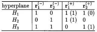
reachable from as the projection of onto is not at the asymptotic decision boundary. Continuing this process for the other two hyperplanes leads to the separability and reach-ability table given in Table I. As is sufficiently separated from the opposite-class states by the two reachable hyperplanes and , there are two bias vectors and for , where is the minimum rate point, and the error region is covered by the half space formed from and . Since is sufficiently separable by a single reachable hyperplane , there is one bias vector for , where is the minimum rate point, and the error region is covered by the half space formed from . For this example, the constructed IS simulation density achieves AE.

[image:5.612.347.507.264.317.2]

Remark 2: The construction procedure for the IS simula-tion density discussed previously, if it can be done, will guar-antee the AE of IS simulation. Strictly speaking, however, AE can only be guaranteed at the asymptotic case. As pointed out in Remark 1, if the SNR is too small, the multiple-hyperplane decision boundary may deviate from the true optimal decision boundary . Shifting the density to the asymptotic deci-sion boundary is then not “optimal.” This is the main source for

Fig. 2. Simulation density construction for the case of binary(M = 2) symbols with a two-tap channel. In this example, there are three Gabriel neighbor pairs(r ; r ); (r ; r ); and (r ; r ). The asymptotic decision boundary is formed from the three corresponding hyperplanesH ; H ; and H . The separability and reachability table for this example is given in Table I.

TABLE I

SEPARABILITY ANDREACHABILITYTABLE FOR THEEXAMPLEGIVEN INFIG. 2

a relatively small IS gain when SNR is small, as can be observed in the simulation results.

Remark 3: Since it is assumed that correct decisions are fed back, the IS simulation procedure considered here provides a lower bound SER for the Bayesian DFE. In practice, it is more useful to provide some upper bound SER and to take into ac-count error propagation caused by incorrect decisions being fed back. However, due to its highly complicated structure, deriva-tion of an upper bound SER for the Bayesian DFE will be ex-tremely difficult, if not impossible. In the lack of any upper bound, the lower bound SER is the only means that can be used to evaluate potential performance of the Bayesian DFE.

B. Numerical Examples

Example 1: The IS technique was simulated for the Bayesian DFE with four-PAM symbols using the three-tap CIR defined by

. The DFE structure was specified by and . The channel state set had states. Five pairs of Gabriel neighbor states were found from the sub-sets and , giving rise to five separating hyperplanes. The separability and reachability table for this example is listed in Table II, from which the required bias vectors were gener-ated. For this example, it is straightforward to verify that the constructed simulation density achieves AE. An inspection of Table II shows that the states to in are sufficiently

..

TABLE II

SEPARABILITY ANDREACHABILITYTABLE FOR THECHANNEL

h = [0:4 1:0 0:6] WITHFOUR-PAM SYMBOLS

separated from the opposite class by the two reachable

hy-perplanes and to are sufficiently separated

from by the two reachable hyperplanes and , and to are sufficiently separated from by the

hyper-plane .

As in [15], the bias vectors were selected with uniform

prob-ability in the simulation with for ,

that is, no attempt was made to optimize the probabilities in (25). For each SNR, iterations were employed, averaging over all the possible states in . Thus, the total samples used for a given SNR were . Fig. 3(a) shows the lower bound SERs obtained using the IS and conventional sampling (CS) simulation methods, respectively. It can be seen that the con-ventional Monte Carlo results for low SNR conditions based di-rectly on the Bayesian DFE of (11) and (12) agreed with those of the IS simulation. The estimated IS gains, which are depicted in Fig. 3(b), indicate that exponential IS gains were obtained with increasing SNRs. It can be seen that for small SNR conditions, the IS gain is relatively small for the reason given in Remark 2. For example, given SNR dB, the IS gain was a modest value of . It should be emphasized that an IS

simula-Fig. 3. (a) Lower bound SERs and (b) the estimated IS gain of the Bayesian DFE for the CIR h = [0:4 1:0 0:6] with four-PAM symbols using conventional sampling (CS) and importance sampling (IS) simulation.

tion is really needed at very low SER or high SNR situations. Under such conditions, the proposed IS simulation technique is extremely efficient. For example, given SNR dB, the SER of the Bayesian DFE with correct symbols being fed back evaluated by the IS technique was approximately with an estimated IS gain of . The CS method could not work under the same SNR condition, and it would require ap-proximately samples to achieve a similar estimation variance.

Example 2: A two-tap channel with

eight-PAM symbols was simulated, and the Bayesian DFE

structure was defined by and . The

channel state set had states. Nine pairs of Gabriel neighbor states were selected from the subsets and , and Table III lists the separability and reachability table for this example. It is straightforward to verify that the constructed simulation density achieves AE. The state is sufficiently separable from the opposite-class by the two reachable hyperplanes and is sufficiently separable from

by the two reachable hyperplanes and is

separable by the two reachable hyperplanes and

is separable by the two reachable hyperplanes and , and to are separable from by the single reachable hy-perplane . As this is a two-dimensional example, the graphic illustration of the simulation density construction can be made and is shown in Fig. 4. Notice the difference between the true optimal decision boundary under a low SNR condition and the asymptotic decision boundary. This explains the relatively small IS gain in the simulation for low SNR conditions.

[image:6.612.80.246.100.486.2]

TABLE III

SEPARABILITY ANDREACHABILITYTABLE FOR THECHANNELh = [0:3 1:0]

WITHEIGHT-PAM SYMBOLS

Fig. 4. Simulation density construction for the channelh = [0:3 1:0] with eight-PAM symbols. Thick solid curve indicates the asymptotic decision boundary, thick dashed curve the true optimal decision boundary for small SNR, and thin lines indicate the bias vectors used in the simulation density.

for each state in , resulting in a total of samples for a given SNR. Fig. 5(a) depicts the lower bound SERs ob-tained using the IS and CS simulation methods, respectively. Again, the conventional Monte Carlo results for low SNR con-ditions agreed with those of the IS simulation. It can be seen from Fig. 5(b) that exponential IS gains were obtained with in-creasing SNRs.

IV. CONCLUSION

A randomized bias technique for IS simulation has been ex-tended to evaluate the lower bound SER of the Bayesian DFE with -PAM symbols. It has been noted that the Bayesian de-cision boundary separating any two neighboring signal classes is asymptotically piecewise linear and consists of several hyper-planes. Furthermore, it has been shown that asymptotically the SER of the Bayesian DFE for the -PAM symbol constellation is a scaled error rate of the equivalent binary Bayesian DFE eval-uated on any two neighboring signal subsets. Although asymp-totic efficiency of the proposed IS simulation method for the general channel has not rigorously been proved, a design proce-dure has been presented for constructing the simulation density that meets the asymptotic efficiency conditions. The SER evalu-ated is under the assumption that correct symbols are fed back, and error propagation is not taken into account. Nevertheless, the method provides a practical means of evaluating the

poten-Fig. 5. (a) Lower-bound SERs and (b) estimated IS gain of the Bayesian DFE for the CIRh = [0:3 1:0] with eight-PAM symbols using conventional sampling (CS) and importance sampling (IS) simulation.

tial performance for the Bayesian DFE under high SNR condi-tions.

REFERENCES

[1] S. U. H. Qureshi, “Adaptive equalization,” Proc. IEEE, vol. 73, pp. 1349–1387, Nov. 1985.

[2] J. G. Proakis, Digital Communications, 3rd ed. New York: McGraw-Hill, 1995.

[3] J. Moon, “The role of SP in data-storage systems,” IEEE Signal

Pro-cessing Mag., vol. 15, pp. 54–72, Apr. 1998.

[4] J. G. Proakis, “Equalization techniques for high-density magnetic recording,” IEEE Signal Processing Mag., vol. 15, pp. 73–82, Apr. 1998.

[5] K. Abend and B. D. Fritchman, “Statistical detection for communica-tion channels with intersymbol interference,” Proc. IEEE, vol. 58, pp. 779–785, May 1970.

[6] D. Williamson, R. A. Kennedy, and G. W. Pulford, “Block decision feed-back equalization,” IEEE Trans. Commun., vol. 40, pp. 255–264, Feb. 1992.

[7] S. Chen, B. Mulgrew, and S. McLaughlin, “Adaptive Bayesian equaliser with decision feedback,” IEEE Trans. Signal Processing, vol. 41, pp. 2918–2927, Sept. 1993.

[8] S. Chen, S. McLaughlin, B. Mulgrew, and P. M. Grant, “Bayesian deci-sion feedback equaliser for overcoming co-channel interference,” Proc.

Inst. Elect. Eng.—Commun., vol. 143, no. 4, pp. 219–225, 1996.

[9] P. J. Smith, M. Shafi, and H. Gao, “Quick simulation: A review of impor-tance sampling techniques in communications systems,” IEEE J. Select.

Areas Commun., vol. 15, pp. 597–613, July 1997.

[10] D. Lu and K. Yao, “Improved importance sampling techniques for ef-ficient simulation of digital communication systems,” IEEE J. Select.

Areas Commun., vol. 6, pp. 67–75, Jan. 1988.

[11] J. S. Sadowsky and J. A. Bucklew, “On large deviations theory and asymptotically efficient Monte Carlo estimation,” IEEE Trans. Inform.

Theory, vol. 36, pp. 579–588, June 1990.

[12] G. C. Orsak and B. Aazhang, “Efficient importance sampling tech-niques for simulation of multiuser communication systems,” IEEE

Trans. Commun., vol. 40, pp. 1111–1118, June 1992.

[image:7.612.45.283.96.393.2]

[14] J. C. Chen, D. Lu, J. S. Sadowsky, and K. Yao, “On importance sam-pling in digital communications—Part I: Fundamentals,” IEEE J. Select.

Areas Commun., vol. 11, pp. 289–299, May 1993.

[15] R. A. Iltis, “A randomized bias technique for the importance sampling simulation of Bayesian equalizers,” IEEE Trans. Commun., vol. 43, pp. 1107–1115, Feb./Mar./Apr. 1995.

[16] S. Chen, “Importance sampling simulation for evaluating the lower-bound BER of the Bayesian DFE,” IEEE Trans. Commun., vol. 50, pp. 179–182, Feb. 2002.

[17] S. Chen and L. Hanzo, “An importance sampling simulation method for Bayesian decision feedback equalizers,” in Proc. 5th Int. Conf. Math.

Signal Process.. Warwick, U.K., Dec. 18–20, 2000.

[18] S. Chen, L. Hanzo, and B. Mulgrew, “Decision feedback equalization using multiple-hyperplane partitioning for detecting ISI-corrupted M-ary PAM signals,” IEEE Trans. Commun., vol. 49, pp. 760–764, May 2001.

[19] S. Chen, B. Mulgrew, E. S. Chng, and G. Gibson, “Space translation properties and the minimum-BER linear-combiner DFE,” Proc. Inst.

Elect. Eng.—Commun., vol. 145, no. 5, pp. 316–322, 1998.

[20] S. Chen, B. Mulgrew, and L. Hanzo, “Asymptotic Bayesian decision feedback equalizer using a set of hyperplanes,” IEEE Trans. Signal

Pro-cessing, vol. 48, pp. 3493–3500, Dec. 2000.

[21] V. Vapnik, The Nature of Statistical Learning Theory. New York: Springer-Verlag, 1995.

[22] S. Chen, S. Gunn, and C. J. Harris, “Decision feedback equalizer de-sign using support vector machines,” Proc. Inst. Elect. Eng.—Vis., Image

Signal Process., vol. 147, no. 3, pp. 213–219, 2000.

Sheng Chen (SM’97) received the Ph.D. degree

in control engineering from the City University, London, U.K., in 1986.