Hyperbolic Velocity Model
Igor Ravve, Zvi Koren Paradigm Geophysical, Herzliya, Israel Email: [email protected], [email protected]
Received March 27, 2013; revised April 29, 2013; accepted May 26, 2013
Copyright © 2013 Igor Ravve, Zvi Koren. This is an open access article distributed under the Creative Commons Attribution License, which permits unrestricted use, distribution, and reproduction in any medium, provided the original work is properly cited.
ABSTRACT
Asymptotically bounded velocity profiles describe the vertical velocity variations in compacted sediments in a more realistic way than unbounded velocity models, and allow presenting the subsurface by a smaller number of thicker lay- ers. The first and the simplest asymptotically bounded model is the Hyperbolic velocity profile proposed by Muscat in 1937, and our paper is an extension of this early study. The Hyperbolic model has an advantage over other bounded models: The velocity increases with depth and approaches the limiting value with a more smooth and gradual rate. We derive the time-depth relationships, forward and backward transforms between the instantaneous velocity profile and the effective models (average, RMS and fourth order average velocities), study the trajectories for pre-critical and post-critical curved rays and derive the equations for traveltime, lateral propagation and arc length. We compare the ray paths obtained with the Hyperbolic model and with the other bounded velocity profiles.
Keywords: Velocity Models; Velocity Transforms; Sediments
1. Introduction
The Hyperbolic velocity model was first proposed by Muscat [1] and published in 1937. However, since then the model was not extensively studied and is unjustifia- bly ignored in the literature. The objective of this re- search is to extend the original study and to correct the inaccuracies. We show the place of the Hyperbolic model among the other asymptotically bounded models, analyze its basic relationships and attempt to develop a complete theory.
Asymptotically bounded velocity models describe the velocity profile in compacted sediments, where the ve- locity gradually increases with depth and eventually ap- proaches a limiting value. These models make it possible to describe a vertical velocity profile with a smaller num- ber of intervals as compared to the classical unbounded models, such as linear velocity vs. depth [2,3], unbounded exponent [4], linear slowness [5], “sloth” (linear varia- tion of slowness squared), e.g., [6], parabolic model [7,8], Faust velocity model [9,10] with a reference depth and different root indices. The unbounded models are de- scribed by two parameters: the instantaneous velocity at the top interface Va and the vertical velocity gradient a at the same level. The Faust model includes also the
root index n, normally . Asymptotically bounded
models require an additional parameter: the limiting value of velocity at infinite depth. Two models of
this family were studied by Ravve and Koren: the Expo- nential asymptotically bounded model [11,12] and the Conic model [13]. The asymptotically bounded profiles can be used, in particular, as velocity trend functions for the constrained velocity inversion with the best (e.g., least-squares) fit of the input data [14]. Examples of as-ymptotically bounded models are presented below. For each model, we first give the original formulation of the velocity profile as it appears in the original works by the authors, and then we convert it to a canonical form in terms of the “standard” parameters and
k
6 n
V
,
a a
V k V. Pa-
rameter V means the instantaneous velocity range,
a
V V V
.
The Hyperbolic velocity model by Muscat [1],
a, const.V z V
z A A
V V z
(1)
In our notation, the Hyperbolic profile reads
Va V 1 . (2)
a
V
V k z
V z
The Exponential velocity model by Muscat [1],
lnz
ln a nst.
a
V V z V V
B V V z V
V ,B co (3)
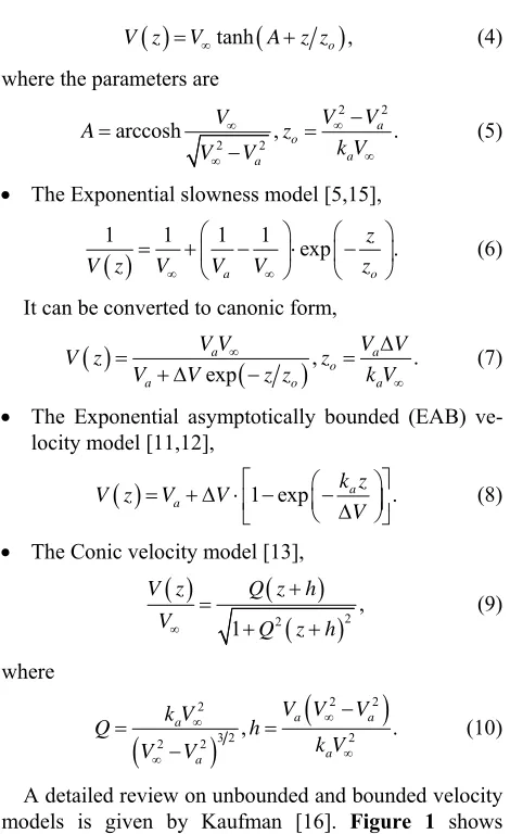
tanh
o ,V z V Az z
(4)where the parameters are
2 2
2 2
arccosh , a .
o a a
V V
V
A z
k V
V V
(5) The Exponential slowness model [5,15],
1 1 1 1 exp .
a o
z
V z V V V z
(6)
It can be converted to canonic form,
,exp
a a
o
a o
V V V V
V z z
V V z z k V
a . (7) The Exponential asymptotically bounded (EAB) ve-
locity model [11,12],
1 exp a .a
k z
V z V V
V
(8) The Conic velocity model [13],
22 ,
1
V z Q z h
V Q z h
(9)
where
2 2
2
3 2 2
2 2 , .
a a
a
a a
V V V
k V
Q h
k V
V V
(10)
A detailed review on unbounded and bounded velocity models is given by Kaufman [16]. Figure 1 shows graphs of the instantaneous velocity vs. depth for the five asymptotically bounded velocity models mentioned above.
For all models, we assume the same velocity profile
parameters: . The ver-
[image:2.595.56.291.76.460.2] [image:2.595.317.517.84.212.2]tical gradients of the velocity vs. depth are plotted in
Figure 2. It is interesting to note that among the five models presented, the Muscat Hyperbolic model (Equa- tion (1) and grey line on the plot) approaches the limiting value in the slowest and the most gradual manner. The “second slow” is the Conic velocity model (red line), and the “third slow” is the EAB model (blue line). An asymptotically bounded model can be characterized by its gradient-velocity relationship, which is actually the governing differential equation of the velocity model.
1
3 km/s, 1 s , 6 km/s
a a
V k V
V
This paper is structured as follows. We define the Hy- perbolic model using 1) the original Muscat [1] formula- tion—depth vs. velocity, 2) the physical parameters: maximum gradient R, length scale and vertical shift h, and 3) the “technical” or geophysical parameters: top
interface velocity Va, top gradient a and asymptotic
velocity . We introduce the dimensionless asymptotic factor
Q
k V
M that simplifies the transform equations. First
0
3
6
9
12
3 3.5 4 4.5 5 5.5
De
pt
h (
k
m
)
Velocity (km/s)
Asymptotically Bounded Velocity Models
6 Conic Velocity Model
EAB Velocity Model Exponential Slowness Exponential Muscat Hyperbolic Muscat
Figure 1. Asymptotically bounded velocity models: Muscat hyperbolic model, Muscat exponential model, the Exponen- tial slowness model, the Exponential asymptotically bounded model and the Conic model: Velocity vs depth. For all mod- els, the profile parameters are: the top interface velocity Va = 3 km/s, the top gradient ka = 1 s−1 and the asymptotic ve-
locity V∞ = 6 km/s.
0 1 2 3 4 5 6 7 8
0 0.1 0.2 0.3 0.4 0.5 0.6 0.7 0.8 0.9 1
Depth (
k
m
)
Vertical Gradient (1/s) Gradient vs. Depth
[image:2.595.328.516.306.433.2]Conic Model EAB Model Exp Slowness Exp Muscat Hyp Muscat
Figure 2. Vertical gradients vs. depth for asymptotically bounded velocity models.
we derive the time-depth and the depth-time relationships. Next we proceed to forward transforms from the instan- taneous velocities to the effective models, such as the average, the RMS and the fourth order average velocity. Then we study the inversion problems, considering the inversion with the instantaneous velocities and gradients, and the inversion with the effective models, i.e., the av-
erage or the RMS velocities given vs. time or depth. Next we comment on the two types of curved rays existing in all asymptotically bounded models, depending on the ini- tial take-off angle, and derive the trajectories of the ray paths for the Muscat velocity profile. For both types of the curved rays we derive the lateral propagation, the tra- veltime and the arc length.
2. The Hyperbolic Velocity Profile
Muscat [1] defined the Hyperbolic model by
a ,V z V
z
A V V z
(11)
from the top interface, a is the top interface velocity, A
is the characteristic distance (scale) that affects the top gradient a, and is the asymptotic velocity. Inverting
Equation (1), we obtain
V
k V
.1
a
V V z A
V z
z A
(12)
The velocity gradient becomes
2d 1 ,
d 1
V V
k z
z A z A
(13)
where V VVa At z0, the top gradient is kka.
Therefore,
a
k V A and A V ka. (14)
Introduce Equation (14) into Equation (13). In our no- tation, the Hyperbolic profile reads
1 a .a
a a
V V V k z
V
V z V V
V k z V k z
a
h
(15) We call values and V the technical parame-
ters of the profile. At a definite height above the earth surface (above the upper interface), where
,
a a
V k
z , the
instantaneous velocity vanishes. According to Equation (15),
.
a a
V V h
k V
(16)
Introduce the absolute frame , where the in- stantaneous velocity vanishes at the origin
z z h
0
z . Pa-
rameter is the shift between the two frames of refer- ence. In the absolute frame, the velocity profile simplifies to
h
,1 1
R h z
Rz V z
Qz Q h z
(17)
where
2and .
a
Qk V V RQV (18)
We call values and the physical parameters of the profile. Note that the linear velocity profile, where the ray trajectories are circular arcs, is a particular case of the Hyperbolic model with and V , in such
way that their product
,
R Q h
V
0 Q
R Q
remains a finite value, and parameter becomes the constant velocity gradient of the linear model. The velocity gradient of the Hyper- bolic model reads
R
2.1 R k z
Qz
(19)
At the absolute origin z0 k
, the velocity gradient reaches its maximum value max . Comparing Equa-
tions (17) and (19), we conclude that
max
1.
V z k z
V k
(20)
Equation (20) is the governing differential equation of the Hyperbolic velocity profile. It can be used to plot the gradient-velocity diagram. Such diagrams for several asymptotically bounded velocity models are studied in Appendix A.
Introduce the normalized (dimensionless) velocity v,
the normalized gradient and the normalized absolute depth ,
ˆ k ˆ
z
ˆ ˆ
, , . (21)
vV V kk R zQz
Note that parameter Q is the reciprocal characteristic
length. With these notations, the Hyperbolic velocity pro- file simplifies to
2ˆ ,ˆ 1
ˆ
1 1 ˆ
z
v k
z z
. (22)
The technical parameters of the velocity profile are re- lated to the physical parameters,
2, ,
1 1
a a
Rh R R
V k V
Qh Qh Q
, (23)
The inverse relationship is
2
2, , . (24)
a a a
a a
k V V V V R
R h Q
k V V
V V
3. Asymptotic Factor
To simplify the equations for velocity transforms, it is suitable to introduce a special parameter M. This pa-
rameter can be defined at any point of the profile, and in particular, at the top and the bottom interfaces of an in- terval,
1 ,
1 ,
1 ,
a
b
M z Q h z
M Qh
M Q h z
(25)
where z is the interval thickness (the vertical distance
between the two interfaces), subscript a is related to the
top interface z0, and subscript b is related to the bot-
tom interface z z. It follows from Equation (25) that
,
a b
a b
V V
M M
V V V V
,
(26)
where a and Vb are the top and bottom instantaneous
velocities, respectively. Next, it follows from Equation (26) that parameter M is the inverse normalized measure
of the difference between the velocity at the given depth level and the asymptotic velocity . Equation (26) can be inverted,
V
V R
1 ,
a a b b
a b
V M V M
V M V M
1. (27)
The velocity gradient is also related to the asymptotic factor,
2,
a b
a b
R
k k R2.
M M
(28) It follows from Equation (25) that
b
a
,b a
a b
V V V
M M
Q
z z V V V V
(29)
and
1 ,
1 .
a a
a
b b
b
V
Qh M
V V
V
Q h z M
V V
(30)
We use Equations (28) and (29) to get the interface gradients, a and , through the increment of the as-
ymptotic factor,
k kb
b a
M M M
,
2 , 2
b a b a
a b
a b
M M V M M V
k k
z
M M
z. (31)
It follows from Equation (31),
2 a , 2 b
b a a a b b
k z k z
M M M M M M
V V
(32) Equations (27) and (29) result in the average gradient on the interval, ave, expressed either through the inter-
face asymptotic factors
k
a
M and Mb, or through the
interface gradients ka and kb,
ave
.
b a b a
a b
a b a b
V V V M M
V k
z z z M M
QV R
M M M M
(33)
Introduction of Equation (28) into Equation (33) leads to
ave a b.
k k k (34)
The average gradient on the interval with the Hyper- bolic velocity profile is the geometric average of the top and bottom interface gradients.
Given the velocity and its gradient at one interface, one can calculate these parameters at the other interface. The calculations can be done either in depth or in time. Four problems of this kind are considered in Appendix C.
4. Depth-Traveltime Relationship
Integrate the slowness to get the vertical traveltime vs. the interval thickness,
0
d d 1 1 d
1
ln .
z h z h z
h h
z z Q
t z
V z V z V Qz
z h z
V QV h
z
(35)
The traveltime equation can be written in terms of asymptotic factors at the top and bottom interfaces, Ma
and Mb. With the use of Equations (25) and (29), we
obtain
1 1
1 ln
1
b
b a a
M
V t z
M M M
, (36)
where the top asymptotic factor Ma is calculated with
Equation (26), and the bottom asymptotic factor Mb
z - with the first equation of Equation Set (32). The interval velocity (local average velocity) through the layer be- tween the interfaces becomesInt .
1 ln
1
b a b b a
a
V z M M
M
V V t M M
M
(37)
To get the vertical distance vs. traveltime we should invert Equation (26), i.e. find Mb
t . Introduction of Equation (29) into (36) results in1
ln .
1
b b a
a M
QV t M M
M
(38)
Equation (38) should be solved for the unknown bottom asymptotic factor Mb,
1 ln 1
1 ln 1 .
b b
a a
M M
M M R
t
(39)
Taking exponent from both sides of Equation (39), we get
1 exp 1
1 exp 1 exp .
b b
a a
M M
M M R
t
(40)
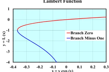
Equation (40) can be solved with the Lambert function,
0
1 1 exp 1 exp ,
b a a
M L M M R t (41)
where notation 0 means the zero branch of the Lambert
function. The Lambert function
L
yL x delivers the
solution of the transcendent equation x y expy, see
Appendix B for details. In terms of the interface velocities, Equation (41) reduces to
0 exp exp .
b a a
b a a
V V V
L R
V V V V V V
t
(42)
After the bottom asymptotic factor Mb or the bottom
interface velocity b is found, the interval thickness can
be established with Equation (29),
b
a
.b a
a b
V V V
M M
z
Q Q V V V V
(43)
5. Hyperbolic and Non-Hyperbolic Moveout
In the absence of the intrinsic anellipticity, the hyperbolic parameter W and the non-hyperbolic parameter H on theinterval are defined as
2
4 3
d d
d d
b b
a a
b b
a a
t z
t z
t z
t z
W V t V z,
.
H V t V z
(44)
Introduce the velocity profile from Equation (17). The hyperbolic parameter W becomes
d d
1 1
ln .
1
b
a
z z h z
z z h
Rz z
W V z
Qz
Q h z
V
V z
Q Qh
(45)
The non-hyperbolic parameter H becomes
3 3 3
3
3 3
3
3 3
2
3
d d
1
3 1 3 1
1 1
1 1
2 1 2 1
1 3
ln .
1 b
a
z z h z
z z h
R z z
H V z
Qz
V V
V z
Q Qh Q Q h z
V V
Q Qh Q Q h z
Q h z
V
Q Qh
2
(46)
With the use of the top and bottom asymptotic factors, the hyperbolic parameter becomes
ln
1
1 ln
b
b a
a
b
b a a
M V
W M M
Q M
M
V z
M M M
.
(47)
Introducing Equation (37) for the traveltime into Equa- tion (47), we obtain the local RMS velocity U over the
interval. By definition, U W t, so
2 2
ln . 1 ln
1
b b a
a b b a
a
M
M M
M U
M
V M M
M
(48)
The non-hyperbolic parameter becomes
3
3
2 2
3 3
1 1 3 ln .
2 2
b a
a b
b
a
a b
V
H M M
Q M M
M V
Q M M M
(49)
With the use of Equation (29), the non-hyperbolic pa- rameter simplifies to
3
2 2
3 3
1 l
2
a b b
a b a b b a a
H V z
M M M
M M M M M M M
n .
(50)
When the parameters of the velocity profile are speci- fied, the top asymptotic factor Ma is a known value. The
bottom asymptotic factor Mb can be presented either vs.
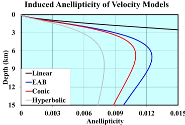
depth (interval thickness) or vs. traveltime. Thus, the hy- perbolic and non-hyperbolic parameters become func- tions of depth or traveltime, accordingly. The anelliptic- ity induced by the vertically varying velocity is defined as the fractional difference between the fourth-order av- erage velocity V4 and the RMS velocity V2,
4 4
4 2
4 2
. 8
V V
V
(51)
Parameter can be also considered as a function of depth or vertical time. For a particular case of a single infinite layer (half-space) with any vertical velocity pro- file,
2
2 4
2 , 4 8 2 .
W H H t W
V V
t t W
(52)
The graph for the induced anellipticity is plotted vs. depth in Figure 3 for three asymptotically bounded velocity models: Exponential, Conic and Hyperbolic. For all the three models, the parameters of the velocity pro- file are: Va3 km/s,
1 and . At the
surface, the anellipticity is zero as there are yet no accu- mulated variations of the instantaneous velocity. The induced anellipticity is always positive. It reaches a maximum value a definite depth and then vanishes at the
1s
a
k V6 km/s
0
3
6
9
12
15
0 0.003 0.006 0.009 0.012 0.015
Depth (km)
Anellipticity
Induced Anellipticity of Velocity Models
[image:5.595.330.514.583.708.2]Linear EAB Conic Hyperbolic
infinity, where the medium velocity is asymptotically constant.
6. Forward Dix Transform
Consider a package of n layers (vertical intervals), where
the nodes (interfaces) are enumerated from zero, and layers are enumerated from 1. Interval n connects nodes
(top interface) and n (bottom interface). The nodal
average velocity V1,n, RMS velocity and fourth-
order average velocity are 1
n
2,n V
4,n V
1, 1 1 1,
1 2 2, 1 1 2
2,
1 4 4, 1 1 4
4,
1
,
,
.
n n n
n
n n
n n n
n
n n
n n n
n
n n
V t z
V
t t
V t W
V
t t
V t H
V
t t
(53)
where tn is the one-way interval traveltime, zn is
the layer thickness, Wn and Hn are the interval hyperbolic
and non-hyperbolic parameters, respectively. For n1 we set 0 in Equation (53). The effective velocities (average, RMS and fourth-order average) can be also defined for any internal point of the interval.
0
t
7. Inverse Dix Transform
Recall that the Hyperbolic velocity profile on the interval is defined by the three parameters: the top interface in- stantaneous velocity a, the top interface gradient a,
and the asymptotic velocity V. We consider that the asymptotic velocity is always given a priori. When the two other parameters, a and ka, are also known, then
velocity transforms are considered forward. When one or both parameters are unknown (with another data speci- fied instead), we deal with the velocity inversion. There are three groups of inverse transforms studied in Appen- dices D, E and F.
V V
k
Appendix D considers the inversion that does not in- volve the RMS velocity. These formulations deal with the instantaneous velocity and its gradient only. We solve a problem where the two velocities are given at the in- terfaces, a and Vb, or—alternatively—the two gradi-
ents, a and b. Another kind of problem is when the
velocity and its gradient are given at the different inter- faces of the interval, i.e. the velocity is given at the top
interface and the gradient—at the bottom interface, a
and b, or vice versa, ka and Vb. We solve also a
problem where the instantaneous velocity is given at the bottom interface and at the intermediate point of the in- terval, b and Vc. These problems are studied both vs.
depth and vs. time.
V k
k V
k
V
Appendix E considers the inversion with the RMS ve-
locity specified at the interfaces vs. depth or time with a single parameter unknown, either Va or a. We con-
sider also a problem with the traveltime specified vs. the interval thickness, also with a single parameter unknown. Finally, we consider the RMS velocity specified vs. both
depth and time, with the two parameters unknown, and .
k
a V a
In Appendix F we study the two-interval inversion. The RMS velocity is given vs. depth or time at the two interfaces and at an internal point of the interval. Alter- natively, depth can be specified vs. traveltime at the three points. Both parameters of the velocity profile are un- known. This is a so-called three-point or two-interval in- version.
k
8. Ray Trajectories
In this section we establish the trajectories of non-verti- cal rays. Due to Snell’s law, in 1D medium the horizontal slowness p is constant, and the ray angle (meas- ured from the vertical axis) becomes
sin pV z . (54) Introduce the ray parameter m,
1 1
,
Q m
pR pV P
(55)
where Q and R are the physical parameters of the Hy-
perbolic velocity profile, is the normalized ray slowness, and m is its inverse value. We call parameter m
“eccentricity of the ray trajectory” as it is very similar to the eccentricity of the hyperbolic and elliptic rays of the Conic velocity model [13]. With Equation (17), the sine of the ray angle becomes
P pV
1
sin ,
1 1
pRz Qz
Qz m Qz
(56) so that the tangent of this angle is
2
2 2 2 2 2
sin tan
1 sin
, 2
Qz
m m Qz m Q z
(57)
where 2 1
m m2. Parameter (the conjugate ec-
centricity squared) may be positive or negative. Intro- duce the dimensionless coordinates,
2
m
ˆ ,ˆ .
xQx zQz (58)
The tangent of the ray angle becomes
2 2 2
ˆ ˆ
1 d
tan .
ˆ
d d
ˆ ˆ
1 2
z x
m z m m z z
dx
z (59)
ˆ ˆ
ˆ ˆd 2 2 2,ˆ ˆ
1 2 c
z z m x x
z m m z
(60)where xc is the constant of integration. This integral
can be reduced to
2 2 2
2
2 2 2
2 2
2 2 2 2
ˆ ˆd
ˆ ˆ
1 2
ˆ ˆ
1 2 ˆ d
.
ˆ ˆ
1 2
z z
z m m z
m
z m m z
m
m z
m z m m z
(61)
To obtain the integral on the right side of Equation (61), we consider two cases, or two ranges of the eccen- tricity: m > 1 (pre-critical rays) and m < 1 (post-critical
rays),
2 2 2
2 2
2
2 2 2
2 2
2
ˆ d
ˆ ˆ
1 2
ˆ
arccosh for 1,
ˆ d
ˆ ˆ
1 2
ˆ
arccos for 1.
z
z m m z
m m m z
m m
m z
z m m z
m m m z
m m
m
(62)
For a limiting case m1 (critical rays),
ˆ ˆ
ˆ ˆd
ˆ 1
1 2ˆ,3 ˆ
1 2
c
z z
z z x x
z
(63)We emphasize that two kinds of rays exist for any monotonously increasing and asymptotically bounded velocity model, and in particular, for the Hyperbolic mo- del. The pre-critical rays that may start on the earth sur- face, propagate to the infinite depth, and their curvature asymptotically vanishes. The post-critical rays have a li- mited propagation depth. Their arc-like trajectories have a finite minimum curvature at the turning point, and these rays return to the earth surface. Note that at any point of the trajectory, the ray path curvature de- pends on the velocity gradient k only,
z pk z
. (64) In particular, the linear velocity model with a constant velocity gradient leads to ray trajectories of constant curvatures, i.e. to the circular arcs.
The critical rays with the unit eccentricity m1 are the limit case between the two types of rays. Their take- off angle (the ray angle at the upper interface) is called the critical angle C. It follows from Equations (54) and
(55) that the critical take-off angle is
arcsin a.
C
V V
(65)
It follows from Equations (61) and (62) that the tra- jectories of the pre-critical and post-critical rays are
2 2 2 2
2 2 2
2 2 2 2
2 2 2
ˆ ˆ
for 1,
ˆ ˆ
ˆ
1 2 arccosh ,
ˆ ˆ
for 1,
ˆ ˆ
ˆ
1 2 arccos .
c
c
m x x
m m z m m m
z
m
m m m
m x x
m m z m m m
z
m
m m m
z
z
(66) At infinite depth, pre-critical rays become asymptoti- cally straight. Equation (57) leads to
2
1 1
tan ,sin .
1 m pV
m
(67)
However, although the slope of these rays converges to a constant value and their curvature becomes infini- tesimal, the pre-critical rays of the Hyperbolic model have no asymptotic straight line, unlike the pre-critical rays of the EAB and the Conic models. The pre-critical, critical and post-critical rays are plotted in Figure 4 for the Hyperbolic, the Conic and the Exponential (EAB) models. Parameters of the velocity profile are the same
0 1 2 3 4 5 6 7 8
0 4 8 12 16 20
De
pth
(
k
m)
Distance (km)
Ray Trajectories Hyp Con EAB
3.00 3.00 3.00 3.75 3.84 3.85 4.20 4.42 4.46 4.50 4.82 4.90 4.71 5.09 5.21 4.88 5.28 5.43 5.00 5.43 5.59 5.10 5.53 5.71 5.18 5.61 5.79
km/s
1 2 3 4 5 6
[image:7.595.319.525.439.569.2]7 8 9
Figure 4. Pre-critical (red lines), critical (green lines) and post-critical (blue lines) ray trajectories for Hyperbolic (lines 1, 4, 7), Conic (lines 2, 5, 8) and EAB (lines 3, 6, 9) velocity models. Pre-critical rays propagate to an infinite depth and become asymptotically straight. Critical ray pro- pagate to an infinite depth, and the ray angle approaches
as above. The three columns of numbers to the right of the plot area are velocities for the three models at the specified depth levels.
9. Maximum Penetration Depth
Pre-critical rays penetrate to infinite depth. The maxi- mum penetration depth of post-critical rays follows from Equation (59). At the turning point, the ray angle π 2, and thus, its tangent becomes infinite. This leads to a quadratic equation with a single positive root,
max
ˆ .
1 m z
m
(68)
Recall that is the dimensionless depth measured from the absolute origin (above the upper interface). The maximum penetration depth in units of length, measured from the upper interface reads
ˆ z
max
1 1
1 sin 1 sin
.
sin sin
a a
a
a C
a
a a C
V V pV
z
k pV
V k
(69)
10. Lateral Propagation, Traveltime and
Arc Length
In a 1D medium, it is convenient to express the lateral propagation distance x, traveltime tS and arc length s
through the ray angle and angle-dependent gradient
k . These relationships are [12,16] (Kaufman, 1953;
Ravve and Koren, 2006)
1 sin d , d
, sin
1 d .
b
a
b
a
b
a
S x
p k
t
k s
p k
(70)
where a and b are ray angles at the departure and the
destination points, respectively. Equations (17) and (19) make it possible to eliminate depth and to express the gradient through the velocity,
22 .
V V
k R
V
(71)
Next we apply Snell’s law and obtain the vertical gradient vs. the ray angle,
21 sin
k R m . (72)
Note that
2
2
2
2
d d sin
d d 1 sin
1 1
, 1 sin 1 sin
d 1
d sin 1 sin
1
,
sin 1 sin 1 sin
S
x Q x
pR
m m
m m
m m
t R
m
m m
m m
(73)
d
ln tan ,
sin 2
(74)
22
d 1 sin
1 d cos , 1
1 sin 1 sin
1
m
m
m
m m
m
.
(75)
The indefinite integral on the right side of this equation essentially depends on the range of the eccentricity m,
resulting in
pre
2 2
pst
2 2
d 1 sin
tan 2 2
arccoth for 1, pre-critical, d
1 sin
tan 2 2
arccot for 1, post-critical.
I
m
m
m
m m
I
m m
m
m m
(76) For the critical ray, m1
2 3
2sin 2 d
,
1 sin 1 sin
cos 3 2 3sin 2
d .
1 sin 3 1 sin
2(77)
Let a and b be the ray angles at the start point and
the destination point of the ray path, respectively. Equation Set (76) can be re-arranged as follows
For the pre-critical rays, m1
pre
2 2
2 2
tan 2
2 arccoth
cos sin
2 arccoth 2 2 ,
sin 2
b
a
b a a b
b a m
I
m m
m
m m
(78)
pst2 2
2 2
tan 2 2
arccot
cos sin
2 2 2
arccot .
sin 2
b
a
b a a b
b a m
I
m m
m
m m
(79)
pre ,a b
I and Ipst
a, b
are functions of theray angles at the endpoints of the path. The following identities were used,
1
arccot arccot arccot ,
1
arccoth arccoth arccoth .
A B
B A
A B A B
B A
A B
(80)
To simplify the notations, we introduce one more function of the ray angles at the endpoints,
cos ,
1 sin
cos sin
2 2
2sin .
2 1 sin 1 sin
b
a
a b
b a a b
b a
a b
J
m
m
m m
(81)
The normalized lateral propagation becomes
2
, ,
, 1
a b a b
m I J
Qx
m
m m
, (82)
The normalized traveltime is
2
2
2
tan 2
ln
tan 2
1 , ,
,
1.
b S
a
a b a b
Rt
m m I m J
m m
(83)
The normalized arc length is
2
, ,
, 1. (84)
a b a b
I m J
Qs
m
m m
C
For the critical rays, , and the departure angle is critical,
1 m
a
. The ray path parameters are,
3 2
3 2
3 2 cos 3 2
1 2
,
1 sin 3 1 sin
1
ln tan 2
1 sin
3sin 2 2 cos 3 2
2
,
3 1 sin
cos 3 2 3sin 2
. 3 1 sin
b
C
b
C
b
C
b
C
S
Q x
R t
Q s
(85)
The current depth can be also expressed through the ray angle. It follows from Equation (17) that
1
1
.
1 1
b a
b a
b a
V
z Q
R V V
V V V V
V V V V
z z
(86)
Recall that
sin ,
V pV
m
V pV (87)
and therefore
sin sin
1 sin 1 sin
1 1
1 sin 1 sin
2
1 sin 1 sin
sin cos .
2 2
b a
b a
b a
b
a b
b a a b
m m
Q z z
m m
m m
m
m m
a
(88)
In Figure 5 we plot the graphs for the traveltime vs. ray path arc length for the pre-critical, the critical and the post-critical rays of the Hyperbolic velocity profile.
The “trigonometric” solution for the lateral propaga- tion and traveltime of the post-critical rays was obtained (in a different form) by Muscat (1937). However, it was not pointed out in this early study that the solution was related to the post-critical rays only, and that the other, “hyperbolic” solution exists for the pre-critical rays (and a “transient” solution for the critical rays, which are the limit case between the two basic types of rays).
Note that for the vanishing or infinitesimal parameter , the shape of the trajectory, the lateral propaga- tion, the traveltime and the arc length of the Hyperbolic model ray path converge to the corresponding character-
0
Q
0 1 2 3 4
0 4 8 12 16
Ti
m
e (
s)
Ray arc length (km)
Ray Traveltime vs Arc Length
[image:9.595.325.521.554.685.2]20 Pre-critical ray Critical ray Post-critical ray
istics of the linear velocity profile. In this case the as- ymptotic velocity V becomes unbounded, so that the
product remains a finite value and converges to a constant gradient of the linear velocity model. The eccentricity m becomes infinitesimal, and
RQV
0
lim lim .
m V
pRV Q
pR
m V
.
(89) Functions I and J from Equations (79) and (81) simplify
to
, cos cos
b a b a
I J
(90) Equation (66) comes to
2 2 2 2 2 2 1.C
xx p R z p R (91)
This is an equation for the circular arc of radius 1 ,
pR
whose center is located at where is the ray slowness. The lateral propagation, Equation (82), becomes
, 0
c
xx z ,
b
p
cos a cos .
pRx (92)
Equation (83) yields the traveltime for this limiting case,
tan 2
ln ,
tan 2
b S
a
Rt
(93)
and finally, Equation (84) for the arc length converges to
.
b a
pRs (94)
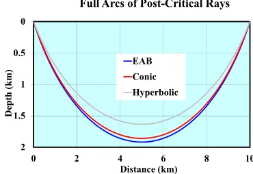
11. Full Arc of Post-Critical Ray
Consider two points on the earth surface, the transmitter and the receiver, located x distance apart. The goal is
to trace the full arc of the post critical turning ray that connects the two points. Note that due to the symmetry of the arc, the ray angle at the destination point b is
related to the take-off angle a ,
π .
b a
(95) Applying Equations (79), (81) and (82), we obtain
2
3 2
sin cos
arccot ,
cos 1 sin 2
a a
a a
m m
m Q x
m
m m m
(96)
where 1 2
m m is the conjugate eccentricity of the
post-critical ray path. Recall that
sin a sin C a .
m V V (97)
Equation (96) simplifies to
2 2
2 2
3 2 2 2
sin sin
arccot .
2 1 sin
sin
C C
C C
m m
m Q x
m m m m
(98)
Equation (98) should be solved numerically for the unknown eccentricity m. To obtain the initial guess, we
assume that the distance x is small. Then the take-off
angle a approaches π 2, and according to Equation
(97), the eccentricity exceeds the sine of the critical angle only slightly. We assume
sin C ,
m m (99)
where m is a small positive value. Next we expand
Equation (98) into the Taylor series and neglect the high order terms,
1 2
2 3
3 2 5 2
2sin 3 13sin
1 sin 6 2sin 1 sin
. 2
C C
C C
m
Q x
m O m
C
(100)
The cubic Equation (100) has a single positive root. For example, for the velocity profile Va3 km/s ,
1 1 s
a
k and V 6 km/s, and the offset , the critical angle becomes
10 km x
π 6
C
. Equation (100) leads to m 0.23
0.7
, and Equation (99) yields the initial guess m 3. Solving Equation (98) with the Newton method, we obtain the eccentricity m . The
take-off angle becomes a . The arcs are plotted in Figure 6 for the three asymptotically bounded velocity models. In the shallow region, the Hy- perbolic model has a smaller vertical gradient (and thus, a smaller curvature) than the Conic and the EAB models, and thus, the Hyperbolic model yields a smaller take-off angle. The ray path arc of the Hyperbolic model passes above the Conic and the EAB arcs.
0.67638
7.67
3 4 0.8319
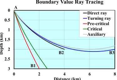
12. Boundary Value Ray Tracing
Given data are the departure point
x za, a
and the ar- rival point
x zb, b
, and the goal is to trace the ray path. The ray path is an explicit function of the eccentricity m,and this parameter is so far unknown. Without any loss of generality, we assume here that xbxa, i.e. that the lat-
eral distance x xb xa and the horizontal ray slowness
0
0.5
1
1.5
2
0 2 4 6 8
Depth (km)
Distance (km)
Full Arcs of Post-Critical Rays
10 EAB
[image:10.595.329.514.579.706.2]Conic Hyperbolic
p are positive. Assume also b a, which is also not a
limitation (one can reverse the endpoints otherwise). Since the ray tracing equations depend on the type of ray, we need to determine, whether the ray is pre-critical or post-critical. For this, one can plot a critical path that starts at the departure point at the critical take-off angle
z z
arcsin
a C V Va
. If the destination point lays to the left from the critical trajectory, then the ray path is pre-critical. The ray path is post-critical if the destination point lays to the right. The critical lateral propagationC x
is delivered by Equation (63), which can be re- arranged as
3 1 1 2
1 1 2
C b b
a
Q x Q z h Q z h
Q z h Q z h
a . (101)
Given the vertical coordinates of the source and the receiver, a and b, we calculate the critical lateral
propagation, and then apply the criterion
z z
pre-critical ray, critical ray, post-critical ray.
C
C
C
x x
x x
x x
(102)
The velocities at the end points of the trajectory and are known values. It follows from Snell’s law that the ray angles at the end points of the trajectory are the functions of the eccentricity alone,
a a
V z Vb
zbsin a ,sin .
a b
V
mV mV
Vb (103)
Note that for the pre-critical rays and for the post critical rays before the turning point, the ray angle is acute, while for the turning rays after the turning point the ray angle is obtuse,
arcsin , before turning point,
π arcsin ,after turning point.
V z z
mV V z z
mV
(104)
Equation (82) relates the lateral propagation x to
the ray angles at the endpoints, which, in turn, depend on the eccentricity according to Equations (103) and (104),
2 ,
1
m I m J m
Q x
m m
(105)
where
2
2
sin 2
cos sin .
2 2
b a
a b
b a a b
V J m
V V V V
m
(106)
Function
a
, bI m I m m . (107)
is delivered by Equations (78) and (79). It was initially defined as a function of the endpoints’ ray angles, but due to Equations (103) and (104) it can be considered as a function of the eccentricity alone. Next we solve nonlinear Equation (105) numerically for the unknown eccentricity m. Then the ray angles at the endpoints can
be established, and the ray path can be plotted with Equa- tion (66). Numerical examples for the boundary value ray tracing with the Hyperbolic velocity profile are presented in Appendix G.
13. Conclusion
The Hyperbolic asymptotically bounded exponential ve- locity model has been studied and compared to other asymptotically bounded models, in particular, the Expo- nential and the Conic. The forward and the inverse ve- locity transforms are derived. The Hyperbolic model allows a better representation of the vertical velocity va- riations in compacted sediments, especially in the case of thick layers. An advantage of the Hyperbolic model is that the instantaneous velocity reaches the asymptotic value in a more slow and gradual fashion, as compared to other asymptotically bounded models. Ray tracing equa- tions have been derived. The ray trajectories, traveltimes and arc lengths have been studied analytically, and the boundary value ray tracing problem have been solved. We have tried to present a complete theory for both ver- tical and non-vertical rays propagating through the Hy- perbolic model. Application of the Hyperbolic velocity distribution enables us to present realistic geological models using fewer parameters, as compared to the clas- sical linear velocity function. We showed that the linear velocity function is a limiting particular case of the Hy- perbolic model.
14. Acknowledgements
We are grateful to Paradigm Geophysical for the finan- cial and technical support of this study and for the per- mission to publish its results.
REFERENCES
[1] M. Muskat, “A Note on Propagation of Seismic Waves,”
Geophysics, Vol. 2, No. 4, 1937, pp. 319-328.
doi:10.1190/1.1438098
[2] M. M. Slotnick, “On Seismic Computations, with Appli- cations, Part I,” Geophysics, Vol. 1, No. 1, 1936, pp. 9-22. doi:10.1190/1.1437084
cations, Part II,” Geophysics, Vol. 1, No. 3, 1936, pp. 299-305. doi:10.1190/1.1437111
[5] M. Al-Chalabi, “Instantaneous Slowness versus Depth Functions,” Geophysics, Vol. 62, No. 1, 1997, pp. 270- 273. doi:10.1190/1.1444127
[6] C. H. Chapman and H. Keers, “Application of the Maslov Seismogram Method in Three Dimensions,” Studia Geo-
physica et Geodaetica, Vol. 46, No. 4, 2002, pp. 615-649.
doi:10.1023/A:1021104820892
[7] C. E. Houston, “Seismic Paths, Assuming a Parabolic Increase of Velocity with Depth,” Geophysics, Vol. 4, No. 4, 1939, pp. 232-236. doi:10.1190/1.1440500
[8] M. Al-Chalabi, “Parameter Non-Uniqueness in Velocity versus Depth Functions,” Geophysics, Vol. 62, No. 3, 1997, pp. 970-979. doi:10.1190/1.1444203
[9] L. Y. Faust, “Seismic Velocity as a Function of Depth and Geologic Time,” Geophysics, Vol. 16, No. 2, 1951, pp. 192-206. doi:10.1190/1.1437658
[10] L. Y. Faust, “A Velocity Function Including Lithologic Variation,” Geophysics, Vol. 18, No. 2, 1953, pp. 271- 288. doi:10.1190/1.1437869
[11] I. Ravve and Z. Koren, “Exponential Asymptotically Bounded Velocity Model, Part I: Effective Models and
Velocity Transformations,” Geophysics, Vol. 71, No. 3, 2006, pp. T53-T65. doi:10.1190/1.2196033
[12] I. Ravve and Z. Koren, “Exponential Asymptotically Bounded Velocity Model, Part II: Ray Tracing,” Geo-
physics, Vol. 71, No. 3, 2006, pp. T67-T85.
doi:10.1190/1.2194897
[13] I. Ravve and Z. Koren, “Conic Velocity Model,” Geo-
physics, Vol. 72, No. 3, 2007, pp. U31-U46.
doi:10.1190/1.2710205
[14] Z. Koren and I. Ravve, “Constrained Dix Inversion,”
Geophysics, Vol. 71, No. 6, 2006, pp. R113-R130.
doi:10.1190/1.2348763
[15] E. Robein, “Velocities, Time-Imaging and Depth-Imaging in Reflection Seismics: Principles and Methods,” EAGE Publications, Houten, the Netherlands, 2003.
[16] H. Kaufman, “Velocity Functions in Seismic Prospect- ing,” Geophysics, Vol. 18, No. 2, 1953, pp. 289-297. doi:10.1190/1.1437871
[17] R. M. Corless, G. H. Gonnet, D. G. Hare, D. J. Jeffrey and D. D. Knuth, “On the Lambert W Function,” Ad-
vances in Computational Mathematics, Vol. 5, No. 1,