Department of Economics University of Southampton Southampton SO17 1BJ UK
Discussion Papers in
Economics and Econometrics
2000
This paper is available on our website
International Trade when Inequality
Determines Aggregate Demand
*
Maurice Kugler
Department of Economics
University of Southampton
Southampton, SO17 1BJ, U.K.
November, 2000
Abstract
The model in this paper characterizes the pattern of international trade, and technological innovation and imitation between industrialized and developing regions, when preferences are nonhomothetic. By and large, models of the dynamics of North-South trade impose the assumption of unit income elasticity for all consumption goods. This assumption is relaxed to incorporate the insight from Engel’s Law: The budget share allocated to necessities falls with income. Since the composition of individual consumption depends on income, aggregate demand for newly invented goods depends not only on the distribution of income across countries but also within countries. To account for the impact of income distribution, preferences are intoduced where consumers rank indivisible goods according to a hierarchy of both needs and desires. In the model, the distribution of wealth is unequal in the less developed country and even in the industrialized country. Then, the composition of the aggregate consumption basket in the integrated economy depends on both inter- and intra-national inequality. Hence, a demand channel is identified through which inequality affects the international trade pattern. Empirical evidence from a panel of bilateral trade data among 58 countries, for which adequate income distribution measures exist, and spanning three decades supports the conjecture that high inequality in a trading partner yields less bilateral trade flows through lower imports, after controlling for both observed and unobserved heterogeneity.
Keywords: Nonhomothetic preferences; inequality; aggregate import demand; pattern of international trade. JEL Codes: F12, F15, O11, O31
1 Introduction
The dynamics of innovation and imitation between industrialized and less developed regions have been investigated in various contexts. The life-cycle structure of the location choice for production of newly invented goods over time, where relatively early manufacturing takes place in industrialized countries and gradually shifts to less developed countries, explored by Vernon (1966), has been formalized in models exploring technology diffusion to emerging economies (See e.g. Grossman and Helpman, 1991). By and large, when it is not supposed that there is a representative consumer, the assumption of unit income elasticity is imposed for all consumption goods. Thus, any impact of income distribution on the level and composition of aggregate demand is ruled out.
In this paper, the model incorporates the fact that income elasticity with respect to newly invented goods is larger than the income elasticity with respect to older ones. The assumption is that more recently introduced goods yield less utility because they satisfy less urgent requirements. They fulfill desires rather than needs. Then wealth distribution determines aggregate demand. This follows from the insight of Engel’s Law: The budget share allocated to necessities decreases with income. As observed by Linder (1961), once the difference in expenditure decisions between rich and poor consumers is acknowledged, the trade pattern between industrialized and less developed regions is determined not only by differentials in technology, factor endowments and income but also by income distribution within each region. To account for the impact of income distribution, we introduce nonhomothetic preferences in an innovation-imitation model of an integrated world economy.
The equilibrium pattern of trade is given not only by technology primitives, factor endowments and relative per capita incomes, that is inter-regional income distributions, as in standard trade theory but also by intra-regional income distributions as pointed out by Linder.
In the model, we assume that the distribution of wealth is unequal in the poor region and even in the prosperous region. This assumption is consistent with the stylized evidence on distribution and development. Hence, our distinction is meant to capture broad modern regional dichotomies of the global North-South or the European East-West type. In particular, we explore the effect of changes in the distribution of wealth within the poor region on the pattern of trade of the integrated economy. The inclusion of nonhomothetic preferences in the model brings about a demand channel through which income distribution, not only between countries but also within trading partners, affects international trade flows. The configuration of global exports will be determined by regional demands for different types of goods.
The effect of wealth inequality in the less developed on trade is ambiguous. On the one hand, since only the rich in the less developed region can afford imported luxurious goods, progressive wealth redistribution leads to a contraction of trade, other things equal. This would occur because the redistribution of wealth is associated with an attendant fall in demand for relatively new goods. On the other hand, if the poor are made wealthier, their range of consumption increases. Then, the varieties of goods produced in the less developed country, and therefore exports, grow. This would occur because the redistribution of wealth is associated with an attendant rise in demand for more recently imitated domestic goods.
2 Related
Literature
Although the impact of international inequality has featured in both the modeling and empirical studies of trade under nonhomothetic preferences, the impact of intra-national inequality has been largely neglected. The present paper aims to bridge this gap in both the theory and empirics of international trade. In this section, we review the existing theoretical and empirical research about the impact of inequality on international trade when the composition of household consumption depends on income, and aggregate consumption for each good on income distibution.
2.1 Theory
In his now classic treatise, Linder (1961) points out that the dependence of the composition of a household’s consumption basket on its income means that aggregate demand for different types of goods is determined by income distribution. In fact, while with homothetic preferences demand for any good only depends on aggregate income, with nonhomothetic preferences the attendant demand for new goods is higher when there are more well off households. Therefore, with fixed costs of innovation, countries with a higher concentration of wealthy households manufacture varieties of the most recent vintages. Some of these varieties are exported from industrialized to less developed countries if enough consumers find them affordable. In particular, bilateral trade will be determined not only by the differences in technology and endowments, as well as the similarity in aggregate incomes, but also by both inter- and intra-national inequality.
introduces transportation costs. Hence, in both models, trade is mostly among countries with higher per capita income. The volume of trade falls with international inequality.
The literature on economic development emphasizes the importance of demand expansion for the adoption of increasing returns technologies that are not viable in small markets. For example, Rosenstein-Rodan (1943) highlights the key role of productive agriculture in generating demand for manufactures and spurring industrialization. But, as Baldwin (1956) points out, the aggregate demand for manufactures may not manifest itself if the wealth generated in agriculture is extremely concentrated. Therofore, intra-national inequality can affect industrial structure.
The idea that the emergence of a middle class is needed, as the source of purchasing power for manufactures, is modeled by Murphy, Shleifer and Vishny (1989). Given that agricultural expansion enlarges the middle class, progressive redistribution unambiguously stimulates industrialization through the expansion of demand that makes it possible for manufacturers of new varieties to cover fixed costs. A role for exports of primary goods is allowed akin to that of agriculture, as generators of the resources that spur industrialization. Luxury imports are considered as detrimental for domestic manufacturing and a negative byproduct of inequality.
By contrast, in the model of the present paper, imports by the rich households in the less developed country are the counterpart of exports to the industrialized country. Without “luxury” imports by the rich, the less developed country manufacturers suffer a drop in their demand because exports cease. Furthermore, international trade facilitates adoption of advanced technologies by manufacturers in the less developed country.
income distribution has impact on industrial structure only through its effect on trade, without any pecuniary externalities of demand to allow for start-up cost coverage. Redistribution from rich to poor consumers in the less developed country reduces exports and imports if the ensuing rise in the terms of trade due to the shift in demand is bounded.
Given that early goods provide more utility and that only the first unit of consumption of each good provides utility, the more rich consumers there are the higher the aggregate demand newer goods. In the model of this paper, like in the model of Murphy, Shleifer and Vishny, redistribution of wealth from the rich to the poor can stimulate demand for domestic manufactures and increase the range of exportable goods in the less developed country. But also, as in Matsuyama’s model progressive redistribution reduces import demand from the less developed country, and therefore total trade flows. Hence, the impact of inequality and redistribution on international trade is ambiguous in the model of this paper.
2.2 Empirics
With regard to the link between the diversity of the consumption bundle and income, Jackson (1984) finds evidence of a positive correlation among household income and variety of goods in its consumption basket. Hunter and Markusen (1988) explore the link between national per capita income and the composition of demand. The estimation of a linear expenditure system for thirty four countries and eleven commodity groups yields a rejection of the null hypothesis of homothetic preferences at significance levels of 1%.
Also, Francois and Kaplan (1996) find that the composition of imports depends on
coefficient of the country running a bilateral trade deficit is negatively correlated total trade flows.
Deardorff (1998) points that if preferences are nonhomothetic and goods with high income elasticity are capital intensive, as in Markusen (1986), the gravity model of bilateral can account for the direction of bilateral flows, as long as the relative per capita income is added as an explanatory variable. But, the prediction that capital abundant countries trade mainly with each other, while capital scarce countries do the same, is not borne out. For example, Frankel, Stein and Wei (1996) find that high-income countries trade disproportionately with all countries, not just other high-income countries. The relevance of intra-national inequality is neglected in estimations of the gravity equation. In the present paper, regressions of the bilateral trade pattern include national inequality.
3
The Building Blocks
In this section the building blocks of the model are laid out. First, the preference structure is specified following Murphy, Shleifer and Vishny (1989) and Zweimueller (1998). We build in Engel's Law. Second, the endowment structure is characterized. Next, the necessary first-order conditions implied by household optimization are used to write the individual and aggregate consumption functions. Finally, the innovation, imitation and manufacturing technologies are characterized.
3.1 Preferences
The model is set up as in Kugler and Zweimueller (1999). The analysis to follow is based on the static equilibrium. The economy is made up of two countries, A and B, populated by LA
and LB inhabitants respectively. Country A is relatively more prosperous and industrialized
Lifetime utility of a household of type h in country i is given by,
( )
ò
∞ − = 0 ) (t e dt Cu
U i t
h i
h δ ,
which is the discounted flow of instantaneous utility from consumption of each infinitely-lived household.
There is a continuum of goods indexed by j∈ℜ+. A hierarchy of necessity and desirability ranks these goods according to their priority. For all goods, we assume that there is indivisibility in consumption and that utility is derived only from the first unit consumed, at each point in time. Households consume conveniences only after basic needs are met. Goods satisfying necessities are indexed in the unit interval, j∈[0,1), and yield one unit of
utility for the first unit consumed. All other goods j≥1 provide amenities for the first unit
consumed, at each moment t∈ℜ+, worth j
1
units of utility.
If prices are not decreasing in j , then each household will consume goods according to the priority specified by the hierarchy. Given equal prices, as j increases each unit of utility from consumption becomes more costly. Hence, no good j≥1 will ever be demanded by a
household until all goods indexed below j have been consumed. Although the decisión-making criterion has a lexicographic structure, the consumption function is continuous and otherwise well-behaved by construction. Note that there exists a continuum of goods and that the index of last good consumed is pari passu a measure of consumption because only one unit of each good is consumed. Indeed, instantaneous utility is given by,
(
( ))
1 1 1 ln ( )) ( 1 t C dj j t C u i h t C j i h i h + = + =
ò
= ,where Ci(t)
h is the highest index of all goods consumed at time t∈ℜ+.
3.2 Endowments
Each household in country A has identical financial asset holdings VA. In country B, there are two types of households, rich and poor. The proportion of poor households is β. Per
capita wealth from financial assets is VB. Each poor household wealth is VB(t) VB(t)
P =α .
Now, ) ( ) 1 ( ) ( )
(t V t V t
V B
R B
P
B =β + −β ,
and therefore, the financial holdings of each rich household are given by,
) ( 1
1 )
(t V t
VB B
R βαβ
− −
= .1
The law of motion of the state variable for each type of household is,
ò
− + = ) ( 0 ) , ( ) ( ) ( ) ( t C i i h i h i h dj t j p t W t rV tV ,
where r is the world interest rate and wages are determined nationally.2 The prices depend
only on the location where the goods are manufactured. Goods manufactured in country A are set as numeraire. Goods manufactured in Country B are cheaper and priced at p<1.
The more recent the invention a good the higher its index j∈ℜ+. The goods manufactured in country A are those which since their introduction have not been imitated in country B.
We assume that N(t) goods have been introduced at time t∈ℜ+ and M(t)imitated. Then
the law of motion of wealth becomes,
î í ì − − + + < − + = otherwise t C t M p t W t rV t M t whenC t pC t W t rV t V i h i i h i h i h i i h i h ), ( ) ( ) 1 ( ) ( ) ( ) ( ) ( ), ( ) ( ) ( ) ( .
We will focus in the case in which (i) households in the relatively prosperous country A purchase all invented varieties, (ii) the rich but not the poor in the less developed country B can afford imported “luxury” goods, and (iii) the poor can afford more than the basic subsistence goods but not all domestically manufactured goods. Hence, we have,
1 ) ( ) ( ) ( )
( = > > > B >
P B
R
A t C t M t C
C t
N .
Since utility is logarithmic, it turns out that the asset distribution is stationary under the present specification of preferences. In particular, the ratio of savings to the value of asset holdings is independent of the level of wealth. The share of wealth of each group is fixed.
3.3 Intertemporal
Optimization
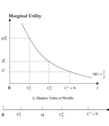
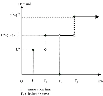
Consumer demand for each household type depends on the range of affordable goods. The demand structure is graphed in Figures 2 and 3.In particular, solving the intertemporal optimization problem of each consumer yields the following consumption functions,
N M p V
W
C A = A + δ A + (1 − ) = (1),
for country A households,
M M p V
W
C B B B
R + − >
− − +
= (1 )
1 1
β βα
δ (2),
for rich households in country B, and
M p V W C B B B P < +
= δα (3),
for poor households.3
2 Labor supply is inelastic.
4
Innovation and Imitation
To complete the specification of the primitives of the model, we provide the elements that determine the cost structure of manufacturing in each region. First, in the rich economy, there is a sunk cost stemming from the resource requirement for innovative design. The marginal cost of producing each unit gives the mark-up equation. Second, in the developing economy, there is a fixed cost associated with reverse engineering. Limit pricing together with the variable cost define the mark-up relationship for imitated products. These technical parameters together with the aggregate demand functions determine the free-entry equilibrium conditions in each region.
4.1 R&D Primitives
Each firm in country A has exclusive use of a blueprint. Perfect intellectual property protection prevails in country A. But, entrepreneurs in country B can reverse engineer a design without compensating the creator. The deployment cost of R&D ventures isF(t)units of labor. Once a design is made, the firm can manufacture each unit using
) (t
A units of labor and acquire a monopoly position for the corresponding good. We assume
symmetry in the technology across goods.
There is an upper bound on the price to be charged by each incumbent firm. We normalize this limit price to unity. The limit on the price is due to potential production by a competitive fringe. Once invented any good can be produced using a “backyard” technology
that has requires 1/WA(t) units of labor to produce each unit of output under constant returns, where A(t)>1/WA(t). Hence, the incumbents’ price determines the reservation wage.
In particular, since we have normalized the price of country A manufactures to unity, the
workers to serve the whole market. No incumbent will ever pay a wage lower than the
reservation level WA(t). With a wage rate WA(t) and a price of unity, the profit flow per unit of output sold is πA =1−A(t)WA(t). The following assumptions summarize the evolution of technical opportunities:
) ( / ) ( ), ( / )
(t f N t At a N t
F = = and WA(t)=wAN(t).
We assume that productivity growth in the relatively prosperous country is driven by innovations. We adopt the simplest way to capture this idea by assuming that the stock of knowledge in the economy can be proxied by the measure of previous innovations N(t)
and the labor input requirement of R&D is inversely related to this measure. Moreover, we assume productivity in final output production, by both incumbents and the competitive fringe, also increases with N(t), which is an index of past manufacturing as well.
Hence, efficiency in R&D and production, both manufacturing and backyard, rise pari passu
with the number of goods introduced. Innovators, entrepreneurs and workers build upon experience of previous successes. The assumption about the impact of new ideas, or designs, on future innovators follows Romer (1990). Learning leading to higher productivity ceases if innovation stops, as in Young (1993). While the wage rate grows with the measure of previous innovations, the profit flow per unit sold remains constant over time as,
πA =1−A(t)WA(t)=1−awA.
4.2 Emulation Primitives
Firms in the less developed country B do not have access to the innovation technology. To become manufacturers they emulate producers from the innovating country A. Imitation requires set-up costs of G(t)units of labor. After a good has been imitated in country B,
necessary to produce one unit of output using the imitation technology and WB(t) is the
wage rate in country B. We will discuss later on the endogenous determination of WB(t).
Technological change for imitation activities evolves analogously to that in innovating activities. In particular, we assume that,
) ( / )
(t g M t
G = and B(t)=b/M(t).
This characterization of the progress of emulation technologies states that efficiency is determined by the history of imitating activities M(t). Productivity in the blueprint imitation
and adaptation process increases as a result of learning from reverse-engineering experience. Successful design copying not only adds to the productivity of further imitation but also leads to more efficient production due to the associated increase in manufacturing experience.
In order to be competitive in the world market, country B producers have to underbid country A firms. The lowest price at which country A firms are willing to sell is their
marginal cost awA. If a country B firm charges a slightly lower price, it can take over the whole world market and drive the country A competitors out of the market. However, the country B firms will only be able to do so if their marginal cost is below that of country A
producers. Or equivalently, we assume awA >bwB, where wB =WB(t)/M(t)denotes the country B wage rate normalized by the measure of previously imitated goods. We obtain the mark-up for imitating producers by invoking limit pricing. In order to capture the market the imitator has to underbid the price of the current producer. The limit price (i.e., the price which drives the country A firm out of the market) is slightly below the marginal cost of the country A firm and the profits per unit sold are thus,
πB = A(t)WA(t)−B(t)WB(t)=awA −bwB.
The free entry condition in country A is given by,
F t W t π L e τ dτ π LA β LB e rτ t dτ
T T A t r A T t A
A( ) ( ) ( (1 ) ) ( )
) ( 2 1 1 − − − − + + −
=
ò
ò
,where T1 is the time at which rich consumers from country B can afford the good
introduced at time t and T2is the time at which that good is imitated an all rents start
accruing to the imitator.
In general, if all variables grow at a common rate γ, we have that,
CB(t)e (T1 t) N(t)
R γ − = and M(t)eγ(T2−t) =N(t), so that, ) ( ) ( ln 1 1 t C t N t T B R − +
= γ and
) ( ) ( ln 1 2 t M t N t
T = +γ− .
If we concentrate in the steady state in which no growth occurs, we have that
δ πA A
A L
fw = .
4.4 Imitation
The free entry condition in country B is given by,
G t W t π L β L e τ dτ π LA LB e rτ t dτ
T B t r B A T t B
B( ) ( (1 ) ) ( ) ( ) ( )
) ( 3 3 − − ∞ − − + + − +
=
ò
ò
,where T3 is the time at which poor consumers from country B can afford the good imitated
In general, if all variables grow at a common rate γ, we have that CB(t)e (T3 t) M(t)
P − =
γ and
) ( ) ( ln 1 3 t C t M t T B P − +
= γ . In particular, if we concentrate in the steady state in which no growth
occurs, we have that
δ β πB( A (1 ) B)
B L L
gw = + − .
Proposition 1
The equilibrium wage in country B falls as the fraction of poor households in country B rises, and as the discount rate gets higher. Also, the wage increases as efficiency, in both imitation and manufacturing, increases in country B, as the cost of manufacturing in country A rises, and as the world population expands.Proof: Using the mark-up expression, we find the wage in country B as,
) ) 1 ( ( ) ) 1 ( ( B A B A A B L L b G L L aw w β δ β − + + − +
= (4),
and the stated results follow directly.
❑
5
The Integrated Economy
In order to characterize the steady state we have to describe the implications of our assumptions on preferences and technology for innovation, imitation, and trade. We assumed that only in country A there is access to the innovation technology. The innovation equilibrium is one where the present discounted value of future profits accruing from an innovation is equal to the fixed cost of discovery. Firms in the country B do not have access to the innovation technology, but there are no barriers to entry in imitation activities. The imitation equilibrium characterization is analogous to the free-entry condition for country A innovators.
The values of innovation and imitation success in steady-state equilibrium were derived under the following conditions. Consumers choose optimally the size and the composition of their consumption basket. The savings are invested in assets until there are no unexploited profit opportunities left, in the sense that neither further incentives to innovate nor to imitate with higher intensity exist. Finally, labor markets have to clear and the current account has to balance. In the steady state without growth, current account balance entails trade balance.
5.1 Resource Balance Constraints
5.1.1 The Less Developed Economy
Since labor supply is inelastic, labor demand is equal to the population in labor market equilibrium. In particular, in country B, work is divided between reverse engineering and production,
L G(t)M (t) B(t)[(L (1 )L )M(t) L CB(t)]
P B B
A
B = + + − β + β
which can be written as,
ú
û ù ê
ë
é + − + +
+ = ) ( ) ( ) 1 ( t M aw t V w L L L b g L A B B B B A
B
γ
β
β
αδ
.
From here, we obtain the steady-state per capita wealth in country B as,
δα
δβα
β
BA A BB aw M t w
L L b
t
V ú −
û ù ê
ë
é − − +
= 1 (1 ) ( )
)
( (5),
5.1.2 The Industrialized Economy
In country A, the labor force is divided into R&D activities and manufacturing, with no “backyard” production in equilibrium. Hence,
LA = F(t)N (t) + A(t)[LAN (t)+ (1−
β
)LBCRB(t)], or, ú ú ú ú û ù ê ê ê ê ë é − + + − + − − + − + + = ) ( ) 1 ( ) ( ) 1 ( ) ( 1 1 ) 1 ( t M aw V w t M aw t V w L L b fL A A A
Proposition 2
The equilibrium per capita wealth in country A rises with the efficiency of manufacturing in country B, with the range of goods produced in country B, and for a given degree of imitation, with the fraction of poor households in country B, because the size of the market for innovations is smaller. Furthermore, the per capita wealth difference among countries falls with the discount rate and the gap between rich and poor in the less developed country.Proof: From (5), we obtain the steady-state per capita wealth in country A as,
[
]
δα
δβα
β
B BB A A B
A V t w
L t M aw bL L b
t
V ( ) = (1− (1− )) − ( ) = ( )+ (6),
and the stated results follow.
❑
Progressive redistribution from rich to poor in the less developed country favors imitators while hurting innovators. While a rise in the discount rate reduces the present discounted value of innovation and imitation. The latter, having a longer horizon, face a sharper fall in value. A drop in imitation, as for example discussed in connection to Proposition 1 when the proportion of poor households rises, affects country A household adversely because their consumption bundles become more expensive. This in turn means that less resources are available for innovation. Somewhat paradoxically, imitation spurs innovation.
5.2 Current Account Balance
As mentioned at the beginning of this section, we will concentrate in the case in which income differences between countries are relatively large, so that the poor in the less developed country cannot afford any imported varieties. M(t) goods are produced in
country B and all these goods are exported as all households in country A can afford them.
numeraire goods produced in country A) is therefore given by awAM(t)LA The demand for exports is given by the number, and wealth, of rich consumers in the country B country. Only this group is assumed to be able to afford imported luxury goods. The level of
consumption of this group is CB(t)
R so the value of exports country B is
B B
R t L
C ( )(1−β) .
In the steady state, the current account balance can therefore be written as,
ú
û ù ê
ë
é + −
− − + −
= ( ) (1 ) ( )
1 1 ) 1 ( )
( w V t aw M t
L aw
L t
M B B A
A A B δ β βα β ,
where the expression in brackets is the optimal consumption of the rich in country B derived in (2).
Proposition 3
The integrated economy will have an equilibrium with international trade if the mark-up of manufactures from country A is sufficiently small and the population of country B relative to that of country A is sufficiently large. Moreover, the degree of manufacturing and exports in country B rises with the wage.Proof: Now, if we plug in the equilibrium wage and per capita assets in country B obtained in equations (4) and (5) from the free-entry and resource balance conditions, we obtain the range of goods produced in country B as,
B w t M ξ + Γ Γ = )
( (7),
where,
[
1 (1 (1 ) )]
(b (1 b))L L b b aw B A A
A − + + + − − − + −
= β α β µ βα
ξ ,
where µA is the price mark-up of goods manufactured in country A, that is the marginal
distribution in country B.4 If the conditions stated in the Proposition are satisfied, then the
last expression is positive and so is the range of goods produced in country B. ❑
Imposing an upper bound on the mark-up of country A amounts to limiting the magnitude of the price of imitated manufactures. This makes them affordable to more consumers, thereby expanding market size for imitators, as does a large population in country B. A large population in country B relative to country A also ensures that there will be some demand for imports from country B, even if the fraction of poor households is large, while households from the industrialized country always consume all goods produced in the less developed country.
The positive feedback between wage rises and manufacturing expansion in the less developed country illustrates the role of nonhomothetic preferences in bringing about a demand channel whereby income distribution determines industrial activity and the pattern of trade. If less inequality induces more production in the less developed country, the industrialized country benefits also because, as explained above, imitation stimulates innovation. Yet, inequality may stimulate growth as imitation follows innovation, and in particular, rises in “luxury’ imports.
5.3 The Pattern of International Trade
In the steady state, this economic system is characterized by the household optimization rules, by the industrial organization among innovators and imitators in equilibrium, by resource balance, and by the balance of trade described in the last section.
Now, we analyze the determinants of international trade. Total trade flows will be derived in terms of the primitives of the model. In particular, we want to explore the impact of the distribution of wealth in country B. Define total trade flows as total exports,
T(t)≡ XB +XA =awAM(t)LA+ B B
R t L
C ( )(1−β) .
Proposition 4
Total trade flows in the integrated economy do not change monotonically with variations in the wealth distribution parameters. While inequality contracts the export supply of the less developed country, it also expands its import demand. The net effect is ambiguous.Proof: Plug in the equilibrium wage and per capita assets in country B obtained in equations (4) and (5), together with the range of production in country B derived in equation 7, to obtain the steady-state total trade flow as,
÷÷ø ö ççè
æ −
+ Γ
Ψ Γ = Γ − Ψ
= M t wBLB wB LB
t T
ξ
) ( )
( ,
where,
B A
A A
A b L aw aw b L
aw (
βα
− (1−βα
)) +[βα
(1− )(1−β
)+ (βα
− (1−β
)(1−βα
))]=
Ψ ,
where the expression for total trade clearly does not vary unambiguously with changes in the
distribution parameters α and β.
❑
The effect of inequality emphasized in the first three propositions points to a contraction in trade due to less imitation, and indirectly less resources for innovation. Proposition 4 introduces a direct effect of inequality in expanding the market for innovators through higher imports from the less developed country. In equilibrium, higher imports from the less developed country entail higher exports to the industrialized country. Hence, in the dynamic model of international trade, nonhomothetic preferences induce two offsetting effects from
6
Evidence on Inequality and Bilateral Trade
In this section, the gravity equation approach is used to analyze the impact of national inequality on international trade flows. The graphical evidence in Figures 4 and 5 hints at the negative effect of inequality on trade, through its impact on import demand. First, preliminary regressions of bilateral import demand and export supply functions are fitted controlling for factors affecting the commercial interaction among the two countries, as well as unobserved heterogeneity of both the importing and exporting country. Second, gravity equations are estimated incorporating national inequality in both countries, and separately controlling for unobserved heterogeneity of the richer and the poorer country respectively.
The database on bilateral trade is described by Frankel and Wei (1995).5 It covers bilateral trade
among 3,906 exporter-importer pairs (63 countries) in 1970, 80, 90 and 92, their nominal GNPs, per capita GNPs and bilateral distance. It comprises information on imports and exports by country of origin, the income and population of each country, as well as characteristics of geographic impediments to trade between pairs of countries, which was matched to data on national inequality for each country. Data on each country’s Gini coefficient for the years in question were available for 58 of the 63 countries from the data compiled by Deininger and Squire.6
6.1 Import Demand and Inequality
The first regression fits import demand on variables capturing observable characteristics affecting bilateral trade and each country’s Gini coefficient, GNP and per capita GNP. The fixed effects estimation controls for unobserved and persistent idiosyncratic characteristics of the country that imports. The results in Table 1 show that while the income distribution of the exporting country is irrelevant, the income distribution of the importing country is significant and negative. That is, inequality lowers import demand. A 1% drop in the Gini coefficient is associated with a 0.65 % rise in imports.
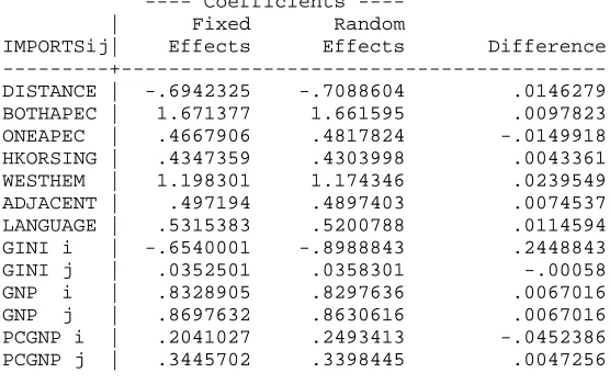
Not only are the regressions controlling for unobserved heterogeneity but also the right hand variables are lagged. Therefore, we cannot attribute this finding the fact that high inequality is positively correlated with other features that hinder imports. The results from the random effects specification, in which unobserved heterogeneity is transitory, are in Table 2. The Hausman specification test in Table 3 of systematic differences in the estimated coefficients rejects the random effects regression in favor of the fixed effects estimation.
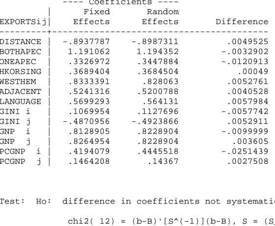
It could be that some countries tend to trade more with countries that have more egalitarian income distributions, independent of their own distribution, for reasons not captured by the regressor variables. In particular, gravitational forces in international trade may have a technical as well as an institutional component. To complement the results in Table 1, an export supply function is fitted with the same regressors but using a fixed effects specification that controls for unobserved and persistent characteristics of the exporting country. The estimated coefficients are in Table 4. Also, a random effects specification assuming transitory unobserved heterogeneity was fitted. The results are in Table 5. While the Hausman specification test in Table 6 clearly favors the fixed effects regression, both estimations show inequality in the exporting country to be highly insignificant.
Inequality in the importing country remains highly significant but the estimate of the elasticity of national imports to the Gini coefficient drops in absolute value to 0.48. A negative effect of inequality on exports is consistent with the model. While progressive redistribution may shrink the fraction of income allocated to rich consumers of “luxury” imports, higher demand for more recent imitated goods by poor consumers induces a rise in both the wage and per capita wealth of country B. Hence, the rich get a smaller share, compared to the initial allocation, from a larger product. The rich can then expand their import consumption range, more than compensating for the smaller share of income allocated to them.
6.2 Total Bilateral Trade and Inequality
It has been established empirically, for the sample of 58 countries under consideration, that inequality in a country lowers its imports without any systematic effect on its exports. Now, it will be ascertained whether the impact on imports carries over to total bilateral trade. For these gravity regressions countries are ranked by per capita income starting with the highest. For any pairing ij, country i always has higher per capita income than country j. The results in Table 7 are obtained by considering persistent effects due to unobserved characteristics of the richer countries. Three new regressors are included. These variables pick up the Gini coefficient, GNP and per capita GNP of the country with a trade deficit in the bilateral exchange. While the income distribution of the rich country is insignificant after controlling for its unobserved characteristics, income inequality in the poor country per se is associated with more total trade. However, if the poor country imports from more than it exports to the rich country, then higher inequality leads to less total international trade flows. The elasticity of total bilateral trade with respect to inequality of countries with lower GNP per capita, and running trade deficits, is –0.28. Bilateral exchange is significantly reduced by inequality in a trading partner but the effect is dampened when compared to the sheer effect on imports.
Finally, the estimation of the gravity equation is performed controlling for unobserved and persistent characteristics of the poorer country in the trade relationship. Inequality in the poor country per se turns insignificant instead of being positively correlated with trade flows. The same happens with GNP and per capita GNP. Now if the country with the lower per capita GNP runs a trade deficit with the richer country, less inequality, a higher national product and a higher income per person will all be associated with more total bilateral trade flows.
7 Conclusions
endowment and cross-regional income differentials, as in the Hecksher-Olin-Samuelson and intra-industry trade models, but also by national income distributions. The incorporation of Engel's Law into the preference structure provides a role for national income distribution to determine the composition of import demand, and therefore the international trade pattern.7
The model of the integrated economy, in which innovation takes place in the industrialized country and imitation in the less developed country, incorporates nonhomothetic preferences. The industrialized country has higher income per capita and a more even income distribution than the less developed country. While inequality may lead to more trade, through higher imports, it can also contract exports by lowering the extent of domestic manufacturing because of lower demand. In equilibrium, redistribution has an ambiguous net effect.
An augmented gravity equation is estimated in which national inequality is included, various types of unobserved heterogeneity are controlled for and a special role for the country running a trade deficit is allowed. The results show that in the sample of 58 countries, for which reliable Gini coefficients are available over three decades, international trade flows are higher when national inequality is lower. The results are quite robust to the control of various types of unobservable heterogeneity, which is generally persistent.
These results demonstrate the role of national income inequality as a crucial, if neglected, determinant of international trade. The aim has been to show how income distribution, within as well as across countries, by shaping the composition of aggregate demand impacts international trade. The significance of inequality in explaining bilateral trade patterns, when preferences are nonhomothetic, has been established both theoretically and empirically.
7 References
Baldwin, R. (1956), “Patterns of Distribution in Newly Settled Regions,” Manchester School, 34 (1): 161-179.
Deardorff (1998), “Determinants of International Trade: Does Gravity Work in a Neoclassical World?,”
in J. Frankel (ed.), The Regionalization of the World Economy, University of Chicago Press.
Francois, J. and S. Kaplan (1996), “Aggregate demand shifts, income distribution, and the Linder
Hypothesis,” Review of Economics and Statistics.
Frankel, J., E. Stein and S.-J. Wei (1996), “Regional Trade Agreements: Natural or Super-Natural,” American Economic Review, 86(2): 52-56.
Grossman, G. and E. Helpman. (1991), Innovation and growth in the global economy, Cambridge, Mass: MIT
Press.
Hunter, L. and J. Markusen (1988), “per capita income as a Basis for Trade,” in R. Feenstra (ed.), Empirical
Methods for International Trade, Cambridge, Mass: MIT Press.
Jackson, L. (1984), “Hierarchic Demand and the Engle Curve for Variety,” The Review of Economics and
Statistics, 66(1): 8-15.
Kugler, M. and J. Zweimueller (1999), “Inequality, Trade Patterns and Long-Run Macroeconomic Performance,” Mimeo, University of Zurich.
Linder, S. (1961), An essay on trade and transformation, Uppsala: Almqvist and Wiksells.
Markusen, J. (1986), ''Explaining the Volumen of Trade: An Ecclectic Approach,'' American Economic
Review, 76(4): 1002-11.
Matsuyama, K. (1999), “A Ricardian Model with a Continuum of Goods under Nonhomothetic Preferences: Demand Complementarities, Income Distribution and North-South Trade,” Math Center Discussion Paper No. 1241, Northwestern University, Evanston, IL.
Ramezzana, P. (2000), “Per Capita Income, Demand for Variety, and International Trade: Linder Reconsidered,” Discussion Paper, London School of Economics.
Rosenstein-Rodan, P. (1943), “Problems of Industrialisation in Eastern and Southeastern Europe,” Economic Journal, 53(2): 202-211.
Romer, P. (1990), “Endogenous Technological Change,” Journal of Political Economy, 98(5): S71-S102.
Vernon, R. (1966), “International investment and international trade in the product cycle,” Quarterly
Journal of Economics, 80(2): 190-207.
Young, A. (1993), “Invention and bounded learning by doing,” Journal of Political Economy, 101(3): 443-472.
8 Appendix
8.1 Wealth
Distribution
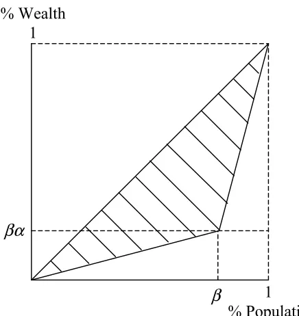
Figure 1
The Gini coefficient is the area between the identity line, perfect equality, and the Lorenz Curve, giving the percentage of wealth owned by a given percentage of the population. The shaded area in the graph corresponds to this measure of inequality. In particular, normalize the are below the diagonal so that,
(
2( )(1 ) (1 )(1 ))
1− β2α+ βα −β + −βα −β
=
Γ ,
and,
β βα
1 % Population % Wealth
1
(
2 1)
(1 )1− βα+ −β −βα =β −α
[image:29.612.187.405.202.433.2]8.2 Consumer
Demand
Figure 2
B P
C B
R
C CA = N
A
λ
B R
λ
B P
pλ
Marginal Utility
J J 1
MU=
λ: Shadow Value of Wealth.
B P
C M CBR CA =N
[image:30.612.90.451.221.639.2]Figure 3
T1
t T2 T3 Time
O LA LA+(1-β) LB
LA+LB
Demand
[image:31.612.100.431.266.574.2]8.2 The
Estimation
Figure 4
Imports and Inequality
-8.00 -5.00 -2.00 1.00 4.00 7.00 10.00
0.20 0.30 0.40 0.50 0.60 0.70
GINI i
IM
PORTSi
j
Figure 5
Total Bilateral Exports and Trading Partner Inequality
-16.00 -13.00 -10.00 -7.00 -4.00 -1.00
0.20 0.30 0.40 0.50 0.60 0.70
GINI i
ln
([X
ij+
X
ji]/[Y
i+
Y
Table 1
Fixed-effects (within) regression Number of obs = 7148
Group variable (i) : i Number of groups = 58
R-sq: within = 0.6995 Obs per group: min = 19
between = 0.2384 avg = 123.2
overall = 0.5647 max = 177
F(13,7077) = 1267.23
corr(u_i, Xb) = 0.0352 Prob > F = 0.0000
---IMPORTSij| Coef. Std. Err. t P>|t| [95% Conf. Interval]
---+---DISTANCE | -.6942325 .0286229 -24.254 0.000 -.7503419 -.6381231
BOTHAPEC | 1.671377 .0953699 17.525 0.000 1.484423 1.85833
ONEAPEC | .4667906 .0500521 9.326 0.000 .3686735 .5649078
HKORSING | .4347359 .1753933 2.479 0.013 .0909127 .7785592
WESTHEM | 1.198301 .0988047 12.128 0.000 1.004615 1.391988
ADJACENT | .497194 .0963623 5.160 0.000 .3082951 .6860929
LANGUAGE | .5315383 .0496536 10.705 0.000 .4342024 .6288741
GINI i | -.6540001 .20824 -3.141 0.002 -1.062213 -.2457874
GINI j | .0352501 .0849377 0.415 0.678 -.1312532 .2017534
GNP i | .8697632 .0133058 65.367 0.000 .8436796 .8958464
GNP j | .8328905 .0128045 64.266 0.000 .8077941 .8579867
PCGNP i | .2041027 .0272805 7.482 0.000 .1506247 .2575807
PCGNP j | .3445702 .0168075 20.501 0.000 .3116224 .3775179
_cons | -5.17441 .374427 -13.820 0.000 -5.908398 -4.440421
---sigma_u | 1.3742681
sigma_e | 1.3317613
rho | .51570432 (fraction of variance due to u_i)
Table 2
Random-effects GLS regression Number of obs = 7148
Group variable (i) : i Number of groups = 58
R-sq: within = 0.6993 Obs per group: min = 19
between = 0.3058 avg = 123.2
overall = 0.5816 max = 177
Random effects u_i ~ Gaussian Wald chi2(13) = 16311.33
corr(u_i, X) = 0 (assumed) Prob > chi2 = 0.0000
---IMPORTSij| Coef. Std. Err. z P>|z| [95% Conf. Interval]
---+---DISTANCE| -.7088604 .0286457 -24.746 0.000 -.765005 -.6527159
BOTHAPEC| 1.661595 .0957685 17.350 0.000 1.473892 1.849297
ONEAPEC | .4817824 .0500387 9.628 0.000 .3837083 .5798566
HKORSING| .4303998 .1763467 2.441 0.015 .0847665 .7760331
WESTHEM | 1.174346 .0990967 11.851 0.000 .9801205 1.368572
ADJACENT| .4897403 .0969302 5.053 0.000 .2997607 .6797199
LANGUAGE| .5200788 .049873 10.428 0.000 .4223296 .6178281
GINI i | -.8988843 .1946852 -4.617 0.000 -1.28046 -.5173084
GINI j | .0358301 .0853804 0.420 0.675 -.1315124 .2031726
GNP i | .8630616 .0133598 64.601 0.000 .8368768 .8892463
GNP j | .8297633 .0133058 65.367 0.000 .8036796 .8558464
PCGNP i | .2493413 .0263411 9.466 0.000 .1977138 .3009689
PCGNP j | .3398445 .0168989 20.110 0.000 .3067232 .3729658
_cons | -5.833791 .3831467 -15.226 0.000 -6.584744 -5.082837
---+---sigma_u | .81288434
sigma_e | 1.3317613
rho | .27143827 (fraction of variance due to u_i)
---Table 3
Hausman specification test
Coefficients
[image:35.612.134.412.237.412.2]----| Fixed Random
IMPORTSij| Effects Effects Difference
---+---DISTANCE | -.6942325 -.7088604 .0146279
BOTHAPEC | 1.671377 1.661595 .0097823
ONEAPEC | .4667906 .4817824 -.0149918
HKORSING | .4347359 .4303998 .0043361
WESTHEM | 1.198301 1.174346 .0239549
ADJACENT | .497194 .4897403 .0074537
LANGUAGE | .5315383 .5200788 .0114594
GINI i | -.6540001 -.8988843 .2448843
GINI j | .0352501 .0358301 -.00058
GNP i | .8328905 .8297636 .0067016
GNP j | .8697632 .8630616 .0067016
PCGNP i | .2041027 .2493413 -.0452386
PCGNP j | .3445702 .3398445 .0047256
Test: Ho: difference in coefficients not systematic
chi2( 13) = (b-B)'[S^(-1)](b-B), S = (S_fe - S_re)
= 49.16
Table 4
Fixed-effects (within) regression Number of obs = 7148
Group variable (i) : i Number of groups = 58
R-sq: within = 0.6895 Obs per group: min = 27
between = 0.3319 avg = 123.2
overall = 0.5523 max = 175
F(12,7078) = 1310.08
corr(u_i, Xb) = 0.0566 Prob > F = 0.0000
---EXPORTSij| Coef. Std. Err. t P>|t| [95% Conf. Interval]
---+---DISTANCE | -.8937787 .0250568 -35.670 0.000 -.9428976 -.8446597
BOTHAPEC | 1.191062 .0927713 12.839 0.000 1.009203 1.372922
ONEAPEC | .3326972 .0481058 6.916 0.000 .2383954 .4269989
HKORSING | .3689404 .1723801 2.140 0.032 .0310239 .7068569
WESTHEM | .8333391 .0957815 8.700 0.000 .6455787 1.0211
ADJACENT | .5299293 .0482527 11.811 0.000 .4353397 .624519
LANGUAGE | .5641316 .0483255 11.674 0.000 .4694146 .6588473
GINI i | .1069954 .2026886 0.528 0.598 -.2903349 .5043258
GINI j | -.4870956 .0867225 -5.617 0.000 -.6570976 -.3170935
GNP i | .8128905 .0128045 64.266 0.000 .7977941 .8379867
GNP j | .8264954 .0127864 64.639 0.000 .8014303 .8515605
PCGNP i | .4194079 .0263698 15.905 0.000 .3677153 .4711006
PCGNP j | .1464208 .0171792 8.523 0.000 .1127444 .1800972
_cons | -2.703383 .3461923 -7.809 0.000 -3.382023 -2.024742
---sigma_u | 1.4745177
sigma_e | 1.2985806
rho | .5631899 (fraction of variance due to u_i)
Table 5
Random-effects GLS regression Number of obs = 7148
Group variable (i) : i Number of groups = 58
R-sq: within = 0.6895 Obs per group: min = 27
between = 0.3592 avg = 123.2
overall = 0.5606 max = 175
Random effects u_i ~ Gaussian Wald chi2(12) = 15684.36
corr(u_i, X) = 0 (assumed) Prob > chi2 = 0.0000
---EXPORTSij| Coef. Std. Err. z P>|z| [95% Conf. Interval]
---+---DISTANCE | -.8987311 .0250477 -35.881 0.000 -.9478237 -.8496386
BOTHAPEC | 1.194352 .0928956 12.857 0.000 1.01228 1.376425
ONEAPEC | .3447884 .0480637 7.174 0.000 .2505852 .4389916
HKORSING | .3684504 .172698 2.133 0.033 .0299686 .7069322
WESTHEM | .828063 .0958331 8.641 0.000 .6402336 1.015892
ADJACENT | .5200788 .049873 10.428 0.000 .4223296 .6178281
LANGUAGE | .5641314 .0483255 11.674 0.000 .4694146 .6588473
GINI i | .1127696 .1954166 0.065 0.948 -.2957791 .2702399
GINI j | -.4923866 .0868892 -5.667 0.000 -.6626863 -.322087
GNP i | .8228904 .0128045 64.266 0.000 .7977941 .8479867
GNP j | .8755891 .1981664 4.570 0.000 .4870476 .9941311
PCGNP i | .4445518 .0258861 17.173 0.000 .3938161 .4952876
PCGNP j | .14367 .0172118 8.347 0.000 .1099355 .1774045
_cons | -3.254213 .3720404 -8.747 0.000 -3.983399 -2.525028
---+---sigma_u | 1.1324436
sigma_e | 1.2985806
rho | .43197738 (fraction of variance due to u_i)
---Table 6
Hausman specification test
Coefficients
[image:38.612.136.417.236.467.2]----| Fixed Random
EXPORTSij| Effects Effects Difference
---+---DISTANCE | -.8937787 -.8987311 .0049525
BOTHAPEC | 1.191062 1.194352 -.0032902
ONEAPEC | .3326972 .3447884 -.0120913
HKORSING | .3689404 .3684504 .00049
WESTHEM | .8333391 .828063 .0052761
ADJACENT | .5241316 .5200788 .0040528
LANGUAGE | .5699293 .564131 .0057984
GINI i | .1069954 .1127696 -.0057742
GINI j | -.4870956 -.4923866 .0052911
GNP i | .8128905 .8228904 -.0099999
GNP j | .8264954 .8228904 .003605
PCGNP i | .4194079 .4445518 -.0251439
PCGNP j | .1464208 .14367 .0027508
Test: Ho: difference in coefficients not systematic
chi2( 12) = (b-B)'[S^(-1)](b-B), S = (S_fe - S_re)
= 45.24
Table 7
Fixed-effects (within) regression Number of obs = 3369
Group variable (i) : i Number of groups = 57
R-sq: within = 0.7857 Obs per group: min = 2
between = 0.4983 avg = 59.1
overall = 0.7410 max = 170
F(16,3296) = 755.10
corr(u_i, Xb) = 0.0905 Prob > F = 0.0000
---TOTTRADEij| Coef. Std. Err. t P>|t| [95% Conf. Interval]
---+---DISTANCE | -.7072502 .0280994 -25.170 0.000 -.7623442 -.6521563
BOTHAPEC | 1.600493 .0847851 18.877 0.000 1.434257 1.76673
ONEAPEC | -.6646207 .2683821 -2.476 0.013 -1.190833 -.1384082
HKORSING | .5198653 .0456675 11.384 0.000 .4303258 .6094048
WESTHEM | .7921349 .0970731 8.160 0.000 .6018052 .9824646
ADJACENT | .5441098 .0923489 5.892 0.000 .3630428 .7251768
LANGUAGE | .6452698 .0472909 13.645 0.000 .5525472 .7379924
GINI i | .3103716 .2712568 1.144 0.253 -.2214773 .8422204
GINI j | .4646067 .0959799 4.841 0.000 .2764204 .652793
GNP i | .9055891 .1981664 4.570 0.000 .5170476 1.294131
GNP j | .7074166 .0163083 43.378 0.000 .6754412 .7393919
PCGNP i | -.6455658 .2152589 -2.999 0.003 -1.06762 -.2235111
PCGNP j | .2310558 .0186839 12.367 0.000 .1944226 .267689
DGINI ij | -.7407607 .1017938 -7.277 0.000 -.9403462 -.5411752
DGNP ij | .0682432 .0177396 3.847 0.000 .0334615 .1030249
_cons | -4.605697 .588925 -7.821 0.000 -5.760393 -3.451001
---sigma_u | 1.2774522
sigma_e | .8610448
rho | .68760642 (fraction of variance due to u_i)
Table 8
Fixed-effects (within) regression Number of obs = 3369
Group variable (i) : j Number of groups = 57
R-sq: within = 0.7914 Obs per group: min = 4
between = 0.5067 avg = 59.1
overall = 0.6440 max = 143
F(16,3296) = 781.49
corr(u_i, Xb) = -0.1368 Prob > F = 0.0000
---TOTTRADEij| Coef. Std. Err. t P>|t| [95% Conf. Interval]
---+---DISTANCE | -.9410296 .0302071 -31.153 0.000 -1.000256 -.8818031
BOTHAPEC | 1.081797 .0999408 10.824 0.000 .8858452 1.27775
ONEAPEC | .408205 .0565621 7.217 0.000 .2973045 .5191055
HKORSING | .4332478 .16986 2.551 0.011 .100206 .7662897
WESTHEM | .4205478 .0968738 4.341 0.000 .2306089 .6104867
ADJACENT | .2766568 .0967818 2.859 0.004 .0868983 .4664153
LANGUAGE | .5493785 .0492445 11.156 0.000 .4528256 .6459313
GINI i | -.2922337 .1014263 -2.881 0.004 -.4910985 -.0933688
GINI j | -.1747095 .1090828 -1.524 0.116 -.3885864 .0391673
GNP i | .8639809 .0151578 56.999 0.000 .8342613 .8937005
GNP j | -.1892749 .1135799 -1.666 0.096 -.4119692 .0334194
PCGNP i | .5688443 .1329551 4.278 0.000 .3081614 .8295273
PCGNP j | -.3876532 .1090828 -1.602 0.109 -.6885864 -.2391673
DGINI ij | -.7435173 .106744 -6.965 0.000 -.9528085 -.534226
DGNP ij | .3759596 .0188669 4.026 0.000 .2896694 .8295111
DPCGNP ij| .5787932 .020327 3.876 0.000 .0538938 .1186479
_cons | -1.183643 .4988506 -2.373 0.018 -2.161731 -.2055545
---sigma_u | 1.2975573
sigma_e | .89689505
rho | .67668962 (fraction of variance due to u_i)