Accurate structural identification for layered composite structures, through a wave and finite element scheme

Accurate structural identification for layered composite structures, through a

wave and finite element scheme

D. Chronopoulosa_{, C. Droz}b_{, R. Apalowo}a_{, M. Ichchou}c_{, W. J. Yan}a,d

a_{Institute for Aerospace Technology & The Composites Group, The University of Nottingham, NG7 2RD, UK} b_{Katholieke Universiteit Leuven, Noise and Vibration Research Group, Division PMA - Celestijnenlaan 300 Leuven, Belgium}

c_{Ecole Centrale de Lyon, 36 Avenue Guy de Collongue, 69134 Ecully Cedex, France}

d_{Department of Civil and Hydraulic Engineering, Hefei University of Technology, Hefei, Anhui 23009, PR China}

Abstract

We present for the first time an approach for identifying the geometric and material characteristics of layered

compos-ite structures through an inverse wave and fincompos-ite element approach. More specifically, this Non-Destructive Evaluation

(NDE) approach is able to recover the thickness, density, as well as all independent mechanical characteristics such

as the tensile and shear moduli for each layer of the composite structure under investigation. This is achieved through

multi-frequency single shot measurements. It is emphasized that the success of the approach is independent of the

employed excitation frequency regime, meaning that both structural dynamics and ultrasound frequency spectra can

be employed. It is demonstrated that more efficient convergence of the identification process is attained closer to the

bending-to-shear transition range of the layered structure. Since a full FE description is employed for the periodic

composite, the presented approach is able to account for structures of arbitrary complexity. The procedure is

ap-plied to a sandwich panel with composite facesheets and results are compared with two wave-based characterization

techniques: the Inhomogeneous Wave Correlation method and the Transition Frequency Characterization method.

Numerical simulations and experimental results are presented to verify the robustness of the proposed method.

Keywords: Structural identification, Non-Destructive Evaluation, Finite Elements, Wave Propagation, Layered

Structures, Ultrasound

1. Introduction

Composites are widely used in modern industry, due to their low density and high dynamic and static

perfor-mances. This goal has led to develop new sandwich structures and composite materials in general, with tailored

properties and a wide range of possible configurations and topologies. However, the verification and Non-Destructive

Evaluation (NDE) of the actual mechanical properties of the assembled layered structure remains a very much open

engineering challenge. Experimental testing and system identification have played important roles in various fields

such as civil engineering, mechanical engineering and aerospace engineering due to their versatile applications such as

Nomenclature

M, K Mass and stiffness matrices of the periodic waveguide

D Dynamics Stiffness Matrix (DMS) of a waveguide’s modelled periodic segment

F Objective function to be minimized

T Transfer matrix of the wave propagation eigenproblem

f Forcing vector for an elastic waveguide

p Vector of structural characteristics to be identified

q Physical displacement vector for an elastic waveguide

x(t) Logged signal vector as a function of time

ρ, h, E, G, v Mass density, thickness and mechanical characteristics of each layer

Lx Dimension of a waveguide’s modelled periodic segment

L, R, I Left, right sides and interior indices

U0 Amplitude of applied excitation signal

cp Wave phase velocity

cg Wave group velocity

f0 Frequency of the applied excitation

k Wavenumber

l, lmax Index corresponding to layer number and total number of structural layers

m, mmax Index corresponding to each measured frequency and total number of measured frequencies

n0 Number of cycles for the Hanning windowed excitation

r f , f e Indices denoting wave characteristics obtained through measurements and the WFE scheme respectively

s Periodic segment positioning index

t Time

x0, x1 Coordinates of the excitation and monitoring locations on the waveguide

Φω,+q ,Φ

ω,−

q Grouped displacement eigenvectors for the positive and negative going elastic waves at frequencyω Φω,+f ,Φ

ω,−

f Grouped forcing eigenvectors for the positive and negative going elastic waves at frequencyω

φ_q,φ_f Displacement and forcing eigenvectors

β Arbitrary structural property

γ Propagation constant and eigenvalue of the wave propagation eigenproblem

assessing system conditions and reconciling numerical predictions with experimental investigations [1, 2, 3, 4, 5, 6].

In a broad context, ’system identification’ refers to the extraction of information about the system behavior directly

from experimental data [7, 8]. Over the past decades, different system identification methods in the time domain

[9, 10, 11], frequency domain [12, 13] and time-frequency domain [14, 15] have been proposed. System identification

has been applied extensively in the field of structural dynamics and it has been proven to be useful in the analysis of

the dynamic behavior of the structure. In the context of structural dynamics, system identification generally includes

modal-parameter identification by extracting the modal data of a structural system such as its natural frequencies,

damping ratio and mode shapes as well as physical-parameter identification by extracting useful information related to

stiffness, mass and damping. Numerous approaches have been developed for system identification including

stochas-tic subspace identification method [16], extended Kalman filter method [17] and Bayesian approaches [18, 19, 20] to

cite a few of them.

The system identification approaches aforementioned are generally based on the measurement of structural

vi-bration information. Nowadays however, several researchers have shown that propagating wave properties can have

a high sensitivity to structural parameters than other structural responses. Therefore, sporadic but consistent efforts

have been directed to extract a system’s structural condition using wave propagation information over the past decade

[21, 22]. However, it is worth mentioning here that rare work reviewed in [21] and [22] are dependent on the model.

Though some efforts [23, 24, 25] have been devoted to inference the model parameters through wave propagation,

they have not resulted in full-fledged applications. Therefore, there is still significant room for further exploration in

system identification by integrating mathematical models of wave propagation. Many methods have been developed

to perform material characterization in composites. On can cite the experimental method for the characterization of

Nomex cores [26], or the vibratory identification technique proposed in Matter et al. [27]. Other methods based on

nu-merical strategies were also developed in [28, 29]. Recently, a Transition Frequency Characterization technique [30]

was developed to perform material identification in sandwich structures, based on the so-called bending-to-shear

con-version effect. However, such methods could not handle more complex topologies often encountered in transportation

industry, despite the considerable progress made on the numerical wave-based models in this field.

The propagation of guided waves in sandwich structures has indeed been the subject of intense research in the

recent years. Traditional analytical methods (i.e. classical plate theory, Mindlin type or first-order shear

deforma-tion theories) typically employed for modelling wave propagadeforma-tion in monolayers can only correctly capture the wave

characteristics in the low frequency range for thick structures. In contrast, Finite Element (FE) based wave methods

assume a full 3D displacement field and are therefore capable of capturing the entirety of wave motion types in the

waveguide under investigation in a very accurate and efficient manner. FE-based wave propagation within periodic

structures was firstly considered in the pioneering work of the author of [31]. The work was extended to two

dimen-sional media in [32]. The Wave and Finite Element (WFE) method was introduced in [33, 34] in order to facilitate the

post-processing of the eigenproblem solutions and further improve the computational efficiency of the method, while

The principal novel contribution of this work is the development of a comprehensive methodology coupling

pe-riodic structure theory to FE in order to identify the characteristics of each individual layer of a composite structure

through experimental measurements on the entire structure. The method is robust and can account for structures of

arbitrary complexity. Both low as well as high frequency excitations can be employed for inverting the structural

prob-lem. It is shown that faster convergence can be acquired around the wave transition region [36, 37] which is a specific

type of wave conversion [38, 39], occurring in sandwich structures subject to flexural vibrations. Both experimental,

as well as numerical case studies are presented in order to validate the exhibited methodology.

The paper is organised as follows: In Sec.2 the FE computational scheme for predicting wave propagation in

multilayered structures is presented and targeted suggestions are made in order to effectively recover the structural

and material characteristics for the structure under investigation. A Hilbert Transform is employed to measure the

time of arrival of the wave pulses and subsequently the propagating wavenumbers. A Newton-like iterative scheme is

eventually employed for minimising the formulated objective function and recovering the mechanical characteristics

of each individual layer through solution of the system of eigenvalue expressions. In Sec.3 several experimental

and numerical case studies are presented for validating the exhibited identification approach. A periodic layered

structure is modelled and multi-frequency single wave shots are excited and measured. The structural and material

characteristics for each layer are then recovered. Conclusions are eventually drawn in Sec.4.

2. An inverse wave and finite element methodology for structural identification

Mathematical modeling can provide a good understanding and form the basis of a characterization process for

a mechanical system. Given the mathematical model, system identification can be implemented by fitting it to that

from experimental testing. In the present paper, the primary focus is to improve structural models by measurements

performed on the real structure using wave propagation measurement data. As a result, one can make inference about

the parameters of a mathematical model based on the observed measurements.

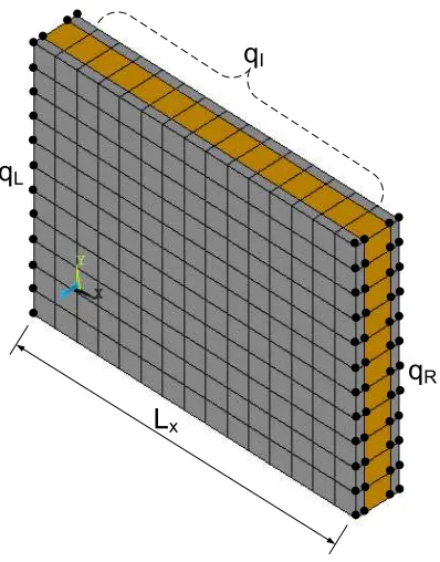
An arbitrarily complex and periodic in the x direction waveguide is illustrated in Fig.1. The structure may comprise

an arbitrary number of layers which may be anisotropic. It is assumed that some of the structural characteristics are

unknown (or even variable over time) and need to be evaluated through a non-destructive evaluation process. The

identifiable properties include the thickness, density as well as the material characteristics of each individual layers.

In the following, a wave and finite element scheme is employed in order to recover the required properties of the

layered structure through the acquired propagating wave data.

2.1. Obtaining the reference wave characteristics

The required data to be extracted and later fed into the structural identification process are the wave phase speeds

(or wavenumbers) of specific wave types propagating within the laminate under investigation. A number of methods

can be employed for exciting and measuring specific propagating wave modes within a composite structure.

q

q

q

L

Figure 1: Caption of the WFE modelled composite waveguide with the left and right side nodes qL, qRbullet marked. The range of interior nodes qIis also illustrated.

in the ultrasound frequency range, while within the structural dynamics spectrum more conventional shaker and

ac-celerometer devices can be employed (see also the experimental study presented in Sec.3.

With regard to numerical calculations, a number of approaches can be employed [42] for exciting the structure

and computing its response at any node. Different wave types can be excited by employing their corresponding

displacement field. Care has to be taken in order to ensure that a sufficiently fine discretization (at least 6-10 elements

per wavelength) has been employed for correctly capturing the propagating waves in the layered structure.

It is hereby assumed that the excitation frequency of the wave packages is known and can be controlled as well

as altered within a certain spectrum. It is generally beneficial to have a range of well separated excitation frequencies

(by at least 50% from each other) in order for the post-processing identification process to converge at a faster rate.

To avoid frequency leakage, a proper signal windowing technique should also be employed. A Hanning window was

chosen as the most appropriate and was employed throughout the results presented in this manuscript. The excitation

signals are quasi-monochromatic burst of amplitude U0, centred around frequency f0and involving a number of n0

cycles. Input signals are windowed so that the input signal is defined by u(t)=U0sin πf0t

n0 !

sin (2πf0t) for 0≤t≤ n0

f0

and u(t)=0 for t>n0 f0.

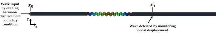
An illustration of the configuration is depicted in Fig.2. The waveguide is excited at a specified central harmonic

signal of frequency f0at a location x=x0and the signal is monitored at location x= x1, after which the signal has

࢞_૙

Wave input by exciting harmonic displacement

boundary condition

࢞_૚

Wave detected by monitoring nodal displacement x

y

Figure 2: Illustration of the suggested configuration for obtaining the reference wave characteristics to be later compared with the WFE ones. All simulations are performed using ANSYS V4.15. Three-dimensional solid brick elements are employed for enhanced accuracy and a minimum mesh density of 15 elements per wavelength is retained.

wavenumbers and group velocities of the excited waves can be easily determined.

Time histories are initially registered at the excitation and monitoring locations. The maximum amplitudes of the

time history signals x(t) are obtained from the Hilbert Transforms H[x(t)] of the acquired signals in the time domain.

Hilbert Transform H[x(t)] of the acquired time signal x(t) is used to evaluate the main attributes of x(t). The signal

envelope is determined at emission, X0and arrival, X1while the time delay is defined by the time difference between

the maximal amplitudes of the envelopes. The total Time of Flight of the wave signal from the point of excitation to

the monitoring point is measured as the time difference t(x1)−t(x0) between the maximum amplitudes of the excited

and the monitored signal envelopes. In ultrasonic NDE, the wavenumber of the wave package is straightforward to

obtain as:

k= ω

cp

(1)

where the phase velocity of the signal cpcan be obtained from its ToF and its propagation distance L. It is noted that

the phase velocity for a non-dispersive wave is equal to its group velocity.

2.1.1. Optimal excitation frequency range for the reference characteristics

As aforementioned, the exhibited scheme can be employed for both in the high as well as the lower frequency

range. It is interesting to note that sandwich laminates comprising a soft core (e.g. honeycomb or foam one), generally

exhibit a so-called transition frequency with regard to their propagating flexural wave speed behaviour.

Kurtze and Watters [43] were the first to observe and develop an asymptotic model for the wave dispersion into

symmetric flat thick sandwich structures. They divided the flexural wave speed of a sandwich panel (frequency-wise)

into three sections, the first characterized by the panel vibrating as a whole, the second by the core’s shear wave speed

and the third by each of the two facesheets vibrating separately and loaded with half of the core mass. In the same

work, it was also shown that the flexural wave type in the sandwich structure has its maximum group velocity value

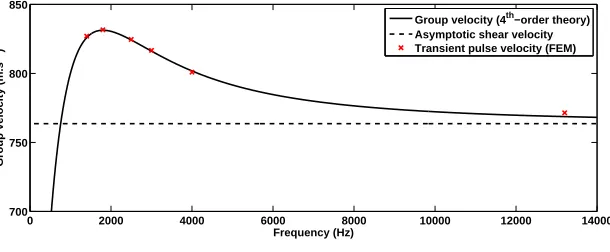
at the transition frequency. As an illustrative example, the group velocities for a typical sandwich structure (to be

investigated in Sec.3) are computed and compared with the transient simulations in Fig.3 (see [30] for details of the

conducted simulation). Since the transition frequency of a sandwich composite is intensely sensitive to its structural

characteristics, it becomes evident that exciting the structure under investigation close to this frequency range can

0 2000 4000 6000 8000 10000 12000 14000 700

750 800 850

Frequency (Hz)

Group velocity (m.s

−1

)

Group velocity (4th−order theory) Asymptotic shear velocity Transient pulse velocity (FEM)

Figure 3: Comparison between theoretical dispersion curves and the velocities obtained by ToF with transient pulse simulations at various frequen-cies. The transition frequency of the sandwich panel is clearly distinguished and characterized by a maximum value for the group velocity. (from [30])

It is noted that this transition for most sandwich laminated occurs well within their ’structural dynamics’ response

range (typically between 2kHz-10kHz). If higher frequencies are excited for the identification process (e.g. ultrasound

range) then obviously exciting the transition range is not feasible, however the identification process will still converge

to the correct properties as shown in Sec.3.

2.2. Structural identification methodology

2.2.1. Considerations on the forward wave FE model

Once again, we consider the periodic complex waveguide illustrated in Fig.1. The propagation constants for

the elastic waves travelling in the x direction can be sought through the forward Wave and Finite Element (WFE)

scheme as described in Appendix A. It is noted that analytical multilayer modelling techniques [44] have also shown

to successfully predict the broadband wave properties for layered structures; however a FE based method is hereby

preferred thanks to its versatility (different numbers of layers and complex material properties are straightforward to

take into account, with no need of altering the modelling approach). Moreover, 3D displacement fields are employed,

therefore retaining accuracy in a broadband frequency regime without any implicit strain field assumptions (such as

the ones used by shear deformation models [45]).

It is obvious that the number of solutions for the formulated eigenvalue problem depends on its size. Most of the

obtained solutions however correspond to either fast decaying, evanescent waves or to numerical artefacts which bare

no physical value. By employing straightforward filtering approaches (typically by comparing the real and imaginary

parts of the obtained wavenumbers as in [46]) the propagating and positive-going wave types can be distinguished

and kept in a separate database for later comparing them with the acquired reference wave characteristics. Using the

obtained wave mode shapesφq(see also Appendix A) the actual wave type can also be categorized (typically flexural,

shear or longitudinal) in order to ensure the fact that the user is always comparing WFE and reference values for the

Due to the large number of numerical artefacts (especially for large models), it is challenging if not impossible

to experimentally reconstruct the vector of eigenvalues and attempt a direct inversion [47] of the eigenvalue

prob-lem of Appendix A (Eq.A.8). Moreover, given the experimental capability of individually exciting just one or two

propagating wave types in a structure it is oftentimes only possible to recover a single eigenvalue per frequency for

the eigenproblem of Eq.A.8. On the other hand, the employment of wave based measurements suggests that

eigen-value data for an unlimited number of frequencies can be extracted, which is the principal advantage of the suggested

method compared to modal based identification techniques.

2.2.2. Formulation of the identification objective function

The advantage of the exhibited WFE approach is therefore the fact that since the excitation frequency is controlled

and known, an unlimited number of eigenvalues (for the same wave) can be extracted for the corresponding number

of frequencies. Since each resulting jtheigenvalue (propagation constants for each wave type) can be expressed as

γj,f e=e−ikj,f eLx (2)

the corresponding wavenumber kjcan be given by

kj,f e=

logγj,f e

−iLx

(3)

which can be directly compared to the reference wavenumber values kj,r f. The objective function of the identification

process to be minimized is then obtained through a least squares approach as

F(p)=

mmax

X

m=1

km,r f −km,f e

2

(4)

with km,r f and km,f e being measured and calculated respectively at frequencyωmfor the same wave type, while p is

the vector of parameters to be identified; in the very general case this is expressed as

p=

Ex,1Ey,1Ez,1vxy,1vxz,1vyz,1Gxy,1Gxz,1Gyz,1h1ρm,1· · ·ρm,lmax

⊤

(5)

for layers l ∈ [1,lmax]. In the above, mmaxis the total number of reference eigenvalues which can be used in the

identification procedure. It is obvious that the minimum required mmaxis equal to the number of parameters to be

identified, however results for additional frequencies will generally improve the precision of the identification process.

An excessive mmaxis undesired, as for each computation ofF, an equivalent number of eigenproblems needs to be

solved.

In order to accelerate the Newton-like iterative scheme, the first (or even the second) gradient of the objective

function∂F

∂βi may be provided for each sought structural propertyβias

∂F ∂βi

=

mmax

X

m=1

2km,f e

∂km,f e

∂βi

−2km,r f

∂km,f e

∂βi

!

It is noted that the set of parameters may be considered to have constrained values (e.g.βi∈[βi,min, βi,max]), again for

practical reasons. In order to compute the gradient of the wavenumber values ∂km,f e

∂βi , an expression of the mass and

stiffness matrices directly as a function of the material and geometric characteristics of each layer is greatly practical,

as derived in Appendix B. By employing the symbolic expressions for the mass and stiffness derivatives∂M ∂βi,

∂K ∂βi the

wavenumber sensitivity ∂km,f e

∂βi can be computed as in [48].

The constrained minimization problem can be implemented within standard mathematics software and nonlinear

optimization algorithms (such as fmincon in MATLAB) can be employed in order to compute the optimal parameter

vector p that minimizesF(p) and corresponds to the identified structural properties. It is stressed that due to the

existence of several local minima inF, a global search algorithm should be employed during the solution process.

The minimum of the encountered solutions is retained as the global set of acquired structural characteristics.

The presented scheme is validated in the following Section through numerical, as well as experimental results.

It is shown that when clear wavenumber measurements are obtained, the approach can be exceptionally accurate.

Moreover, the procedure can be applied within a rational amount of time (especially if only one or two structural

parameters are to be sought) using conventional low-cost computing equipment. The generic iterative procedure of

the post-processing identification process is presented in Algorithm 1.

Algorithm 1 Newton-like iterative scheme for identifying the parameters of a layered structure

1: Input measured reference wave characteristics. Determine total number of local minima to be investigated and evaluated. Define identification criterion for objective functionF

2: i←1 Input structural parameters for initial design to be evaluated

3: Substitute new set of structural parameters in symbolic expressions of M, K, ∂K ∂βi,

∂M

∂βi and formulate the

corre-sponding matrices for the periodic unit cell of the layered design under investigation

4: Solve the eigenproblem of Eq.A.8 for design i. Compute WFE wave velocities and wavenumbers

5: ComputeF and the sensitivity values ∂F

∂βi for each structural parameterβito be recovered 6: if dF <Solution convergence criterion then

7: Solution corresponds to a local minimum

8: ifF <Identification criterion then

9: Solution corresponds to global identification solution and process can end

10: else

11: Radically alter the structural parameters and go to Step 3

12: end if

13: else

14: Use∂F

∂βi in order to alter structural parameters for converging towards a local minimum. i←i+1 (next solution

step). Go to Step 3

ŝŶƉƵƚƉŽŝŶƚ

ŵŽŶŝƚŽƌŝŶŐƉŽŝŶƚ

x

Time (s) 10-4

0 0.2 0.4 0.6 0.8 1 1.2 1.4 1.6 1.8 2

N

o

rm

a

lis

e

d

a

m

p

lit

u

d

e

-1 -0.5 0 0.5 1

y

ŝŶƉƵƚƐŝŐŶĂů

Time 10-4

0 0.2 0.4 0.6 0.8 1 1.2 1.4 1.6 1.8 2

N

o

rm

a

liz

e

d

A

m

p

li

tu

d

e

-1 -0.5 0 0.5 1 1.5

ŵŽŶŝƚŽƌĞĚƐŝŐŶĂů

Figure 4: General representation of the ToF measurements. The pulse input is generated using an excitation device at the input point while the time delay is measured at the monitoring point. Note that better results are obtained when no edge reflections are interfering with the registered pulse.

3. Numerical and experimental case studies

3.1. Numerical validation of the identification scheme

3.1.1. Monolayer case study

The first numerical case study relates to identifying the thickness, density and Young’s modulus for a monolayer

metallic structure under investigation. The properties exhibited under Structure I (see Table 1) are employed for the

monolayer case-study which is modelled by 3D solid elements in ANSYS V14.5. A longitudinal pressure wave

exci-tation is numerically imposed at a cross section of the modelled structure. A general presenexci-tation of the measurement

process is depicted in Fig.4).

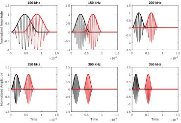
The propagating waveform is depicted in Fig.5 for six wave pulses of different frequencies. As expected, negligible

dispersion occurs for all six pulses, thanks to the high number of cycles n0employed for the Hanning window process,

as well as to the non-dispersive nature of pressure waves. It is clear that the absence of reflected and converted waves

at high frequencies allows a reliable determination of the wave envelope characteristics. It is stated that a

quasi-monochromatic burst is hereby assumed as excitation which may however not always be realistic. For structures

under real operating conditions a number of impediments may exist. These could be related to the quality and feasible

amplitude of the signal (good signal to noise ratio is needed) as well as to the excitation bandwidth which in reality is

never monochromatic. Moreover, operational conditions (mainly temperature as well as pressurization effects) may

alter the wave propagation properties of a certain modelled structure. As is the case with several fields of applied

research, a comprehensive uncertainty quantification needs to be performed before applying this methodology under

×10-4

0 0.5 1 1.5

Normalized Amplitude

-1 -0.5 0 0.5 1

1.5 100 kHz

×10-4

0 0.5 1 1.5

-1 -0.5 0 0.5 1

1.5 150 kHz

×10-4

0 0.5 1 1.5

-1.5 -1 -0.5 0 0.5 1

1.5 200 kHz

Time ×10-4

0 0.5 1 1.5

Normalized Amplitude

-1.5 -1 -0.5 0 0.5 1

1.5 250 kHz

Time ×10-4

0 0.5 1 1.5

-1.5 -1 -0.5 0 0.5 1

1.5 300 kHz

Time ×10-4

0 0.5 1 1.5

-1.5 -1 -0.5 0 0.5 1

1.5 350 kHz

Figure 5: Time acquisition at x=0 (black curves) and x=3cm (red curves) with the wave envelopes depicted in the monolayer structure. The number of cycles is n0=9. The ToF is measured at the maximal amplitude of Hilbert transform (solid lines) signal.

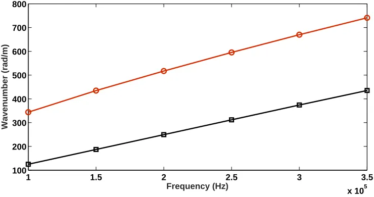
Six wavenumber measurements are recovered for an equivalent number of different ultrasonic frequencies, namely

from 100kHz to 350kHz with a step of 50kHz. The reference wave characteristics related to the recovered wavenumber

values are shown in Fig.6. These are retained for comparison with the WFE obtained results for the same propagating

wave type which will form the objective function of the identification problem. The same process is repeated for a

flexural wave propagating within the monolayer structure with the results also presented in the same Figure.

Once the reference wave characteristics km,r f are established, the objective functionF can be established as a

function of the structural properties to be identified E,ρand h. A single element is employed for the formulation of

the WFE model which results in very fast eigenproblem solutions for Eq.A.8. An identification criterion equal to 10

is employed (suggesting that any local minimum with a value less than that would be considered as a solution). The

minimization process was completed in 58 iterations each of which lasted approximately 8 seconds, resulting in a

total computation time of 460s on a conventional laptop device. This suggests that employing dedicated optimization

software and high-performance computing equipment would radically reduce this amount of post-processing. The

final value of the objective function when pressure wave measurements were employed was of the order of 10−1_{. The}

second best identified solution gave an objective function value at the order of 101, therefore confirming the optimality

of the result. The identified parameters are exhibited in Table 1 and are in excellent agreement with the ones initially

used in the full FE model (maximum divergence is considerably less than 1%). The result therefore validates the

1 1.5 2 2.5 3 3.5 x 105 100

200 300 400 500 600 700 800

Frequency (Hz)

Wavenumber (rad/m)

Figure 6: Reference wavenumber values obtained through a numerical solution of the full FE model for the monolayer structure. Results for a pressure propagating wave () and a flexural propagating one ().

also be identified; however due to the low sensitivity exhibited by the propagating wavenumbers to this structural

parameter, the time required for the process to successfully converge is much greater.

3.1.2. Layered composite case study

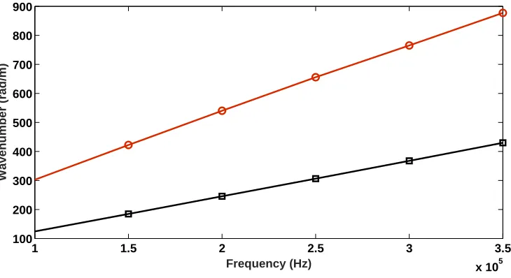
A similar process was followed for extending the calculations to a layered composite structural configuration.

The properties for each layer are given as Structure II (lower facesheet), Structure III (core layer) and Structure IV

(upper facesheet) in Table 1. Once again, a pressure as well as a flexural wave excitation was imposed at a specific

cross-section of the modelled structure. A Hanning window was applied at all pulses with n0=9. The results for six

wave pulses of different frequencies are presented in Fig.7.

In order to find out the maximum number of parameters that can be identified within a rational amount of time

for the multilayer structure, we run the identification procedure for three, four, five and six unknown parameters. The

WFE model this time comprised three FEs (one for representing each structural layer). The identification criterion

was again set equal to 10. It was observed that the processes with five and six unknown parameters never converged

to a satisfactory value of the objective function after 18,000s of post-processing time (5 hours). This is due to the

existence of an important number of local minima that needed to be investigated by the fmincon algorithm. None of

the derived local solutions however had a value close to zero.

The identification process did converge when four parameters were considered unknown (ρII, Gxz,III, Ex,IV and

hIV) with the corresponding indices taken as in Table 1. The minimization process converged after 137 iterations

each of which lasted approximately 14 seconds, resulting in a total computation time of 1950s on a laptop device.

The properties identified through the results corresponding to the pressure wave are again presented in Table 1. Very

1 1.5 2 2.5 3 3.5

x 105 100

200 300 400 500 600 700 800 900

Frequency (Hz)

Wavenumber (rad/m)

Figure 7: Reference wavenumber values obtained through a numerical solution of the full FE model for the multilayer structure. Results for a pressure propagating wave () and a flexural propagating one ().

divergence again not greater that 1%), while the final value of the objective function was equal to 5.34. It is evident that

incorrect wavenumber measurements will radically increase the value of the calculated objective function, therefore

leading to a non-convergent problem. An experimental approach is employed in the following section in order to

further extend the validation process.

3.2. Structural identification through experimental measurements for a layered composite

The experimental validation is based on experimental set-up developed in. In this section, the proposed

identifi-cation strategy is applied to a sandwich structure, and results are compared with the ones obtained in Droz et al. [30]

from IWC method, static experiments and the Transition Frequency Characterization.

The structure is a rectangular sandwich plate measuring 60 cm×288 cm, placed in a horizontal position as depicted

in Fig.(8). The structural response is measured using a Polytec laser vibrometer and is transmitted to the acquisition

system in order to compute the structural impedance at various points of the panel. The panel was excited using a

shaker, controled by the Polytec acquisition system and adhered to the structure through a force sensor.

The constitutive materials are a 10 mm-thick Nomex honeycomb core involving a 3.2 mm cell size, while

prop-agation is considered in the W-direction. The sandwich’s skins are 0.6 mm-thick Hexforce with multi-axial,

carbon-reinforced fibres. The density of the skins given by the manufacturer isρs =1451 kg.m−3and the core’s density is

ρc=99 kg.m−3.

Static measurements conducted on the layered structure provides the following mechanical characteristics for the

Young’s modulus of the facesheets and the shear modulus of the core along the investigated direction:

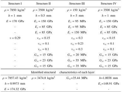
Table 1: Properties of numerically modelled structural layers and identified characteristics through the inverse WFE scheme

Structure I Structure II Structure III Structure IV

ρ=7850 kg/m3 ρ=3500 kg/m3 ρ=150 kg/m3 ρ=3500 kg/m3

h=1 mm h=0.5 mm h=5 mm h=1 mm

E=170 GPa Ex=150 GPa Ex=95 MPa Ex=150 GPa

- Ey=85 GPa Ey=95 MPa Ey=85 GPa

- Ez=85 GPa Ez=150 MPa Ez=85 GPa

v=0.29 vxy =0.15 vxy=0.3 vxy=0.15

- vxz=0.1 vxz=0.23 vxz=0.1

- vyz=0.1 vyz=0.3 vyz=0.1

- Gxy=15 GPa Gxy=20 MPa Gxy=15 GPa

- Gyz=23 GPa Gyz=55 MPa Gyz=23 GPa

- Gxz=15 GPa Gxz=35 MPa Gxz=15 GPa

Identified structural characteristics of each layer

ρ=7857.43 kg/m3 ρ=3474.8 kg/m3 Gxz=35.44 MPa h=1.0038 mm

h=0.9973 mm - - Ex=148.91 GPa

-Figure 8: Photo of the structure used to retrieve experimental wavenumbers.

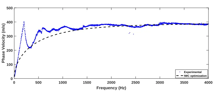
The shaker is used to produce the harmonic excitation at the edge of the plate while the laser vibrometer is used to

measure normal displacement field at the surface, along a 50 cm line of 66 points. The IWC method [49] is employed

to estimate the propagating flexural wavenumbers in the plate. The frequency range of interest spans 0 and 4000 Hz.

The phase velocities obtained by the IWC method are shown in Fig.9. Material properties obtained from the IWC

characterization [30] are:

EIWC=62 GPa and GIWC=37.8 MPa

0 500 1000 1500 2000 2500 3000 3500 4000 Frequency (Hz)

0 100 200 300 400 500

Phase Velocity (m/s)

Experimental IWC optimization

Figure 9: Flexural phase velocities obtained in the main direction of the plate. Inaccurate results are usually expected in the low frequencies for the IWC method. The convergence however increases with frequency, providing approximated material properties and a good correlation with analytical results.

The method proposed in Sec.2 is now applied to estimate the two mechanical characteristics mentioned above.

Pulse measurements are post-processed to retrieve the phase velocities at selected frequencies. Note that the extraction

in the considered frequency range, this is not always the case in higher frequencies. Additionally, the 1 m distance

required in this experimental set-up is due to the low wavenumbers of flexural waves in the sandwich panel. This

distance could be considerably reduced if ultrasonic waves are employed to retrieve local dynamic properties.

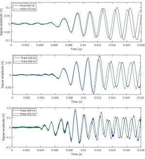
The pulse generation at frequency fn involves at least 10 cycles to limit dispersion effects occurring at these

frequencies and is controlled by the PSV Laser using a triggering procedure. The response is measured at 1 m from

the source for a selected number of frequencies between 500 Hz and 1500 Hz. The time signals are averaged at least

30 times to reduce experimental noise. Noteworthy, the group velocity can also be derived from measured phase

velocities and wavenumbers. Measured pulses are shown in Fig.10 at 6 different frequencies close to the transition

bandwidth.

0 0.002 0.004 0.006 0.008 0.01 0.012 0.014 0.016 0.018

Time (s)

-0.1 -0.05 0 0.05 0.1

Signal amplitude (V)

Puse 550 Hz Pulse 575 Hz

0 0.002 0.004 0.006 0.008 0.01 0.012 0.014 0.016 0.018

Time (s)

-0.05 0 0.05

Signal amplitude (V)

Pulse 625 Hz Pulse 650 Hz

0 0.002 0.004 0.006 0.008 0.01 0.012 0.014 0.016 0.018

Time (s)

-0.2 -0.1 0 0.1 0.2

Signal amplitude (V)

Pulse 900 Hz Pulse 925 Hz

Figure 10: Measured pulse signals at acquisition point.

Note that a refined frequency sampling was used in [30] to evaluate the transition frequency at 880 Hz, and retrieve

the following material characteristics:

ETFC=69.8 GPa and GTFC=36.5 MPa

Generate wave pulses at frequencies

{ 1, ..., n}

Measure Time Of Flight at each

frequency

Derive frequency dependent wave dispersion characteristics

Specify unknown parameters

{ 1, ..., r}

Compute k-space from WFEM

Evaluate fitting with experimental solutions

Apply Newton algorithm: new parameters

{ 1, ..., r}(i+1)

Optimized material parameters { 1, ..., r}(i)

yes

no

Figure 11: Experimental procedure for the WFE-based model updating strategy.

above, the WFE iterative process is formed and the properties of the panel are identified through the presented,

Newton-like minimization scheme. The process depicted in Fig.11 and detailed by Algorithm 1 was programmed

and executed with the experimentally obtained flexural wavenumbers serving as the reference measured values. The

structural parameters to be identified are the Young’s modulus of the facesheet and the shear modulus of the core in

the direction of wave propagation. A new design was therefore generated after each iteration, taking into account the

first derivative ofF. After converging to a minimum ofF, the final value of the objective function was compared to

the identification criterion. If the identification condition was not satisfied, a drastically altered design was evaluated

by the iterative algorithm. Three elements comprise the WFE model which results in very fast model updating and

eigenproblem solutions for Eq.A.8. An identification criterion equal to 10 was employed while the minimization

process converged in 91 iterations each of which lasted approximately 14 seconds, resulting in a total computation

time of 1274s on a conventional laptop device.

The identified Young’s modulus for the skins of the laminate and the shear modulus of the honeycomb core in the

direction under investigation are computed as:

EWFE=69.5 GPa and GWFE=37.1 MPa

which are both in very good agreement with the values provided by the other methods mentioned above, therefore

experimentally validating the exhibited computational scheme.

4. Conclusions

In this work we have developed and applied a new identification technique based on FE modelling and the

prop-erties of propagating waves in multilayered structures. The principal contribution resulting from this work is a robust

numerical NDE procedure for recovering effective structural parameters of complex, layered composites. It can be

(i) The method is able to extract layer characteristics including thicknesses, densities, tensile and shear moduli for

each individual layer and is robust enough to be applied in a broadband frequency range. Case studies elaborating

on both ultrasonic as well as low frequency ranges were presented. In the ultrasound range the wave characteristics

are straightforward to extract through the measured wave envelope, while in the low frequency regime dedicated

techniques can be employed such as the IWC approach.

(ii) The exhibited scheme was validated through comparison with experimental results as well as through full FE

transient response predictions. Excellent agreement is observed for the identified structural parameters.

(iii) It was shown that faster convergence of the post-processing identification algorithm was attained within the

so-called wavenumber transition spectrum where the bending-to-shear transition phenomenon can be easily captured

using the WFE method.

(iv) It is emphasized that the proposed wave-based method has significant advantages compared to modal

identifi-cation approaches. More precisely the accuracy of the structural parameters is not altered by the presence of uncertain

boundaries since the data is obtained locally, through single-shot measurements. This is a considerable advantage

compared to a number of stationary and other existing methods, since it can then be applied in situ and without

requir-ing additional samplrequir-ing of the structure. The use of unlimited and user-selected excitation frequencies can effectively

increase the number of parameters to be identified through the inverse wave modelling, resulting in a significant

increase of the method’s robustness in a broadband frequency sense.

(v) The principal drawback of the presented approach is the required computational effort. This can range from

negligible (when a single structural parameter is sought) to intense, when typically more than three parameters are

to be identified and several iterations need to be completed before the Newton’s scheme converges to the desired

solution. Providing expressions of the wavenumber sensitivity to the investigated structural parameters under

investi-gation can accelerate the convergence process. Drastic computational savings can be attained by a-priori solving the

WFE forward model for a fine grid of variables and using a neural-network type approach for extracting the desired

parameters; this is currently a topic of further research.

Acknowledgements

The authors would like to gratefully acknowledge the H2020 ITN Marie-Curie project GA-721455 ’SAFE-FLY

EID’, as well as the EPSRC thematic doctoral programme ’Waves in Complex Media’ for the financial support.

References

[1] S. Chen, S. A. Billings, W. Luo, Orthogonal least squares methods and their application to non-linear system identification, International Journal of control 50 (1989) 1873–96.

[4] C. Papadimitriou, D.-C. Papadioti, Component mode synthesis techniques for finite element model updating, Computers & structures 126 (2013) 15–28.

[5] E. Chatzi, C. Papadimitriou, Identification methods for structural health monitoring, CISM International Centre for Mechanical Sciences, Courses and lectures (ISSN 0254-1971 567 (2016).

[6] I. Antoniadis, G. Glossiotis, Cyclostationary analysis of rolling-element bearing vibration signals, Journal of sound and vibration 248 (2001) 829–45.

[7] G. Kerschen, K. Worden, A. F. Vakakis, J.-C. Golinval, Past, present and future of nonlinear system identification in structural dynamics, Mechanical systems and signal processing 20 (2006) 505–92.

[8] K.-V. Yuen, Bayesian methods for structural dynamics and civil engineering, John Wiley & Sons, 2010.

[9] E. N. Chatzi, A. W. Smyth, Particle filter scheme with mutation for the estimation of time-invariant parameters in structural health monitoring applications, Structural Control and Health Monitoring 20 (2013) 1081–95.

[10] M. N. Chatzis, E. N. Chatzi, A. W. Smyth, On the observability and identifiability of nonlinear structural and mechanical systems, Structural Control and Health Monitoring 22 (2015) 574–93.

[11] K.-V. Yuen, L. S. Katafygiotis, Bayesian time–domain approach for modal updating using ambient data, Probabilistic Engineering Mechanics 16 (2001) 219–31.

[12] C. Devriendt, P. Guillaume, The use of transmissibility measurements in output-only modal analysis, Mechanical Systems and Signal Processing 21 (2007) 2689–96.

[13] W.-J. Yan, W.-X. Ren, Operational modal parameter identification from power spectrum density transmissibility, Computer-Aided Civil and Infrastructure Engineering 27 (2012) 202–17.

[14] T. Kijewski, A. Kareem, Wavelet transforms for system identification in civil engineering, Computer-Aided Civil and Infrastructure Engi-neering 18 (2003) 339–55.

[15] A. Robertson, K. Park, K. Alvin, Extraction of impulse response data via wavelet transform for structural system identification, Journal of vibration and acoustics 120 (1998) 252–60.

[16] B. Peeters, G. De Roeck, Reference-based stochastic subspace identification for output-only modal analysis, Mechanical systems and signal processing 13 (1999) 855–78.

[17] J. N. Yang, S. Lin, H. Huang, L. Zhou, An adaptive extended kalman filter for structural damage identification, Structural Control and Health Monitoring 13 (2006) 849–67.

[18] J. L. Beck, Bayesian system identification based on probability logic, Structural Control and Health Monitoring 17 (2010) 825–47. [19] W.-J. Yan, L. S. Katafygiotis, A novel bayesian approach for structural model updating utilizing statistical modal information from multiple

setups, Structural Safety 52 (2015) 260–71.

[20] K.-V. Yuen, L. S. Katafygiotis, Bayesian fast fourier transform approach for modal updating using ambient data, Advances in Structural Engineering 6 (2003) 81–95.

[21] Z. Su, L. Ye, Y. Lu, Guided lamb waves for identification of damage in composite structures: A review, Journal of sound and vibration 295 (2006) 753–80.

[22] S. S. Kessler, S. M. Spearing, C. Soutis, Damage detection in composite materials using lamb wave methods, Smart Materials and Structures 11 (2002) 269–75.

[23] C.-T. Ng, M. Veidt, A lamb-wave-based technique for damage detection in composite laminates, Smart materials and structures 18 (2009) 07400–6.

[24] C. Ng, M. Veidt, L. Rose, C. Wang, Analytical and finite element prediction of lamb wave scattering at delaminations in quasi-isotropic composite laminates, Journal of Sound and Vibration 331 (2012) 4870–83.

[25] G. Yan, A bayesian approach for damage localization in plate-like structures using lamb waves, Smart Materials and Structures 22 (2013) 03501–2.

Structures 94 (2012) 2017–24.

[27] M. Matter, T. Gm ¨ur, J. Cugnoni, A. Schorderet, Identification of the elastic and damping properties in sandwich structures with a low core-to-skin stiffness ratio, Composite Structures 93 (2011) 331–41.

[28] M. Schwaar, T. Gm ¨ur, J. Frieden, Modal numerical–experimental identification method for characterising the elastic and damping properties in sandwich structures with a relatively stiffcore, Composite Structures 94 (2012) 2227–36.

[29] D. Jiang, D. Zhang, Q. Fei, S. Wu, An approach on identification of equivalent properties of honeycomb core using experimental modal data, Finite Elements in Analysis and Design 90 (2014) 84–92.

[30] C. Droz, O. Bareille, M. N. Ichchou, A new procedure for the determination of structural characteristics of sandwich plates in medium frequencies, Composites Part B: Engineering 112 (2017) 103–11.

[31] D. J. Mead, A general theory of harmonic wave propagation in linear periodic systems with multiple coupling, Journal of Sound and Vibration 27 (1973) 235–60.

[32] R. Langley, A note on the force boundary conditions for two-dimensional periodic structures with corner freedoms, Journal of Sound and Vibration 167 (1993) 377–81.

[33] B. R. Mace, D. Duhamel, M. J. Brennan, L. Hinke, Finite element prediction of wave motion in structural waveguides, The Journal of the Acoustical Society of America 117 (2005) 2835–43.

[34] J.-M. Mencik, M. Ichchou, Multi-mode propagation and diffusion in structures through finite elements, European Journal of Mechanics-A/Solids 24 (2005) 877–98.

[35] B. Mace, E. Manconi, Modelling wave propagation in two-dimensional structures using finite element analysis, Journal of Sound and Vibration 318 (2008) 884–902.

[36] C. Droz, Z. Zergoune, R. Boukadia, O. Bareille, M. Ichchou, Vibro-acoustic optimisation of sandwich panels using the wave/finite element method, Composite Structures 156 (2016) 108–14.

[37] Z. Zergoune, M. Ichchou, O. Bareille, B. Harras, R. Benamar, B. Troclet, Assessments of shear core effects on sound transmission loss through sandwich panels using a two-scale approach, Computers & Structures 182 (2017) 227–37.

[38] V. K. Chillara, C. J. Lissenden, D. E. Chimenti, L. J. Bond, D. O. Thompson, Guided wave mode conversions across waveguide transitions: A study using frequency domain finite element method, in: AIP Conference Proceedings, volume 1581, AIP, pp. 308–15.

[39] C. Droz, J.-P. Lain´e, M. Ichchou, G. Inqui´et´e, A reduced formulation for the free-wave propagation analysis in composite structures, Composite Structures 113 (2014) 134–44.

[40] E. Brignoli, M. Gotti, K. H. Stokoe, Measurement of shear waves in laboratory specimens by means of piezoelectric transducers (1996). [41] I. J. Collison, T. Stratoudaki, M. Clark, M. G. Somekh, Measurement of elastic nonlinearity using remote laser ultrasonics and cheap optical

transducers and dual frequency surface acoustic waves, Ultrasonics 48 (2008) 471–7.

[42] G. C. Cohen, Q. H. Liu, Higher-order numerical methods for transient wave equations, The Journal of the Acoustical Society of America 114 (2003) 21–.

[43] G. Kurtze, B. G. Watters, New wall design for high transmission loss or high damping, J.Acoust.Soc.Am. 31 (1959) 739–48.

[44] S. Ghinet, N. Atalla, H. Osman, The transmission loss of curved laminates and sandwich composite panels, The Journal of the Acoustical Society of America 118 (2005) 774–90.

[45] J. Reddy, C. Liu, A higher-order shear deformation theory of laminated elastic shells, International Journal of Engineering Science 23 (1985) 319–30.

[46] D. Chronopoulos, M. Ichchou, B. Troclet, O. Bareille, Computing the broadband vibroacoustic response of arbitrarily thick layered panels by a wave finite element approach, Applied Acoustics 77 (2014) 89–98.

[47] M. T. Chu, Inverse eigenvalue problems, SIAM review 40 (1998) 1–39.

[48] D. Chronopoulos, Design optimization of composite structures operating in acoustic environments, Journal of Sound and Vibration 355 (2015) 322–44.

Structures 30 (2008) 2591–604.

[50] J. M. Renno, B. R. Mace, Calculation of reflection and transmission coefficients of joints using a hybrid finite element/wave and finite element approach, Journal of Sound and Vibration 332 (2013) 2149–64.

[51] C. A. Felippa, R. W. Clough, The finite element method in solid mechanics, American Mathematical Society, 1970.

Appendix A. The forward wave and finite element modelling approach

Linear elastic wave propagation is considered in the x direction of the arbitrarily layered structural waveguide of

Fig.1. The problem can be condensed using a transfer matrix approach as in [33]. The frequency dependent Dynamic

Stiffness Matrix (DMS) of the waveguide’s periodic segment can be partitioned with regard to its left/right sides and

internal DoF as

                

DLL DLI DLR

DIL DII DIR

DRL DRI DRR

                                  qL qI qR                  =                  fL 0 fR                  (A.1)

with q the displacement and f the forcing vectors. Using a Guyan-type condensation for the internal DoF the problem

can be expressed as

         

DLL−DLID−_II1DIL DLR−DLID−_II1DIR

DRL−DRID−_II1DIL DRR−DRID−_II1DIR

                   qL qR          =          fL fR          (A.2)

Assuming that no external forces are applied on the segment the displacement continuity and force equilibrium

equa-tions at the interface of two consecutive periodic segments s and s+1 give

qs_L+1=qs_R

f_Ls+1=−fs R

(A.3)

Using Eqs.(A.2),(A.3) the relation of the displacements and forces of the left and right sides of the segment can

be written as

        

qs_L+1

f_Ls+1          =T         

qs_L

f_Ls          (A.4)

and the expression of the symplectic transfer matrix T can be written as

T=          

D11 D12

D21 D22          

[2 j×2 j]

(A.5)

with

D11=−(DLR−DLID−_II1DIR)−1(DLL−DLID−_II1DIL)

D12=(DLR−DLID−II1DIR)−1

D21=−DRL+DRID−II1DIL+

+(DRR−DRID−II1DIR)(DLR−DLIDII−1DIR)−1(DLL−DLID−II1DIL)

D22=−(DRR−DRID−II1DIR)(DLR−DLID−II1DIR)−1

With a wave propagating freely along the x direction, the propagation constantγ = e−ikLx _{relates the right and left}

nodal displacements and forces by

qs R=γq

s L

fs R=−γf

s L

(A.7)

By substituting Eqs.A.3, A.7 in Eq.A.4, the free wave propagation is described by the eigenproblem

γ          qs L fs L          =T          qs L fs L          (A.8)

whose eigenvaluesγw and eigenvectors φw =

         φq φf          w

solution sets provide a comprehensive description of the

propagation constants and the wave mode shapes for each of the elastic waves propagating in the structural waveguide

at a specified angular frequencyω. Both positive going (withγ+

wandφ+w) and negative going waves (γw−andφ − w) are

sought through the eigensolution. Positive going waves are characterised [50] by

|γ+

w|≤1,

ℜ(iωφ+_f⊤φ+_q)<0 if|γ+

w|=1

(A.9)

stating that when a wave is travelling in the positive x direction its amplitude should be decreasing, or that if its

amplitude remains constant (in the case of propagating waves with complete absence of attenuation), then there is

time averaged power transmission in the positive direction.

Appendix B. Structural FE matrices expressed directly as a function of layer mechanical characteristics

A linear solid FE is hereby considered as shown in Fig.12. Following the isoparametric notation introduced in

[51] the geometry of the element is described as

                 x y z                  =                 

x1 x2 x3 x4 x5 x6 x7 x8

y1 y2 y3 y4 y5 y6 y7 y8

z1 z2 z3 z4 z5 z6 z7 z8

                                                                        N1 N2 N3 N4 N5 N6 N7 N8                                                        (B.1)

X Y Z

L

L

L

Figure 12: The considered cuboid solid FE

                 ux uy uz                  =                 

ux1 ux2 ux3 ux4 ux5 ux6 ux7 ux8

uy1 uy2 uy3 uy4 uy5 uy6 uy7 uy8

uz1 uz2 uz3 uz4 uz5 uz6 uz7 uz8

                                                                        N1 N2 N3 N4 N5 N6 N7 N8                                                        (B.2)

Linear shape functions are assumed for the element

N1=1₈(1−ξ)(1−η)(1+µ)

N2=1₈(1−ξ)(1−η)(1−µ)

N3=1₈(1−ξ)(1+η)(1−µ)

N4=1₈(1−ξ)(1+η)(1+µ)

N5=1₈(1+ξ)(1−η)(1+µ)

N6=1₈(1+ξ)(1−η)(1−µ)

N7=1₈(1+ξ)(1+η)(1−µ)

N8=1₈(1+ξ)(1+η)(1+µ)

(B.3)

k= Z 1 −1 Z 1 −1 Z 1 −1

B⊤DB|J|dηdξdµ (B.4)

while the element mass and damping matrices m, c can be determined as

m= Z 1 −1 Z 1 −1 Z 1 −1

N⊤ρmN|J|dηdξdµ (B.5)

c= Z 1 −1 Z 1 −1 Z 1 −1

N⊤γN|J|dηdξdµ (B.6)

with N=                 

N1 0 0 · · · N8 0 0

0 N1 0 · · · 0 N8 0

0 0 N1 · · · 0 0 N8

                 (B.7)

whileρmis the mass density of the material andγthe material damping coefficient. It is also noted that

B=                                        

∂N1

∂x 0 0

∂N2

∂x · · ·

∂N8

∂x 0 0

0 ∂N1

∂y 0 0 · · · 0

∂N8

∂y 0

0 0 ∂N1

∂z 0 · · · 0 0

∂N8

∂z

∂N1

∂y

∂N1

∂x 0

∂N2

∂y · · ·

∂N8

∂y

∂N8

∂x 0

0 ∂N1

∂z

∂N1

∂y 0 · · · 0

∂N8

∂z

∂N8

∂y

∂N1

∂z 0

∂N1

∂x

∂N2

∂z · · ·

∂N8

∂z 0

∂N8

∂x                                                                                                ux1 uy1 uz1 ux2 · · · ux8 uy8 uz8                                                        (B.8)

The Jacobian matrix of the element is

J=                        ∂x ∂ξ ∂y ∂ξ ∂z ∂ξ ∂x ∂η ∂y ∂η ∂z ∂η ∂x ∂µ ∂y ∂µ ∂z ∂µ                        (B.9)

D−1=                                                      1 Ex

−vxy

Ex

−vxz

Ex

0 0 0

−vyx

Ey

1

Ey

−vyz

Ey

0 0 0

−vzx

Ez

−vzy

Ez

1

Ez

0 0 0

0 0 0 1

Gxy

0 0

0 0 0 0 1

Gyz

0

0 0 0 0 0 1

Gxz                                                      (B.10)

The assumption of the undeformed FE being a rectangular parallelepiped is hereby adopted. The coordinates

x1,x2,x3,x4,x5,x6,x7,x8, y1,y2,y3,y4,y5,y6,y7,y8, and z1,z2,z3,z4,z5,z6,z7,z8,can then be replaced by Lx,Ly,Lzin

the expression of B. The generic expression for m is thus given as

m=(ρLxLyLz)                                                                                                                                                                                      

1/27 0 0 1/54 0 0 1/108 0 0 1/54 0 0 1/54 0 0 1/108 0 0 1/216 0 0 1/108 0 0

0 1/27 0 0 1/54 0 0 1/108 0 0 1/54 0 0 1/54 0 0 1/108 0 0 1/216 0 0 1/108 0

0 0 1/27 0 0 1/54 0 0 1/108 0 0 1/54 0 0 1/54 0 0 1/108 0 0 1/216 0 0 1/108

1/54 0 0 1/27 0 0 1/54 0 0 1/108 0 0 1/108 0 0 1/54 0 0 1/108 0 0 1/216 0 0

0 1/54 0 0 1/27 0 0 1/54 0 0 1/108 0 0 1/108 0 0 1/54 0 0 1/108 0 0 1/216 0

0 0 1/54 0 0 1/27 0 0 1/54 0 0 1/108 0 0 1/108 0 0 1/54 0 0 1/108 0 0 1/216

1/108 0 0 1/54 0 0 1/27 0 0 1/54 0 0 1/216 0 0 1/108 0 0 1/54 0 0 1/108 0 0

0 1/108 0 0 1/54 0 0 1/27 0 0 1/54 0 0 1/216 0 0 1/108 0 0 1/54 0 0 1/108 0

0 0 1/108 0 0 1/54 0 0 1/27 0 0 1/54 0 0 1/216 0 0 1/108 0 0 1/54 0 0 1/108

1/54 0 0 1/108 0 0 1/54 0 0 1/27 0 0 1/108 0 0 1/216 0 0 1/108 0 0 1/54 0 0

0 1/54 0 0 1/108 0 0 1/54 0 0 1/27 0 0 1/108 0 0 1/216 0 0 1/108 0 0 1/54 0

0 0 1/54 0 0 1/108 0 0 1/54 0 0 1/27 0 0 1/108 0 0 1/216 0 0 1/108 0 0 1/54

1/54 0 0 1/108 0 0 1/216 0 0 1/108 0 0 1/27 0 0 1/54 0 0 1/108 0 0 1/54 0 0

0 1/54 0 0 1/108 0 0 1/216 0 0 1/108 0 0 1/27 0 0 1/54 0 0 1/108 0 0 1/54 0

0 0 1/54 0 0 1/108 0 0 1/216 0 0 1/108 0 0 1/27 0 0 1/54 0 0 1/108 0 0 1/54

1/108 0 0 1/54 0 0 1/108 0 0 1/216 0 0 1/54 0 0 1/27 0 0 1/54 0 0 1/108 0 0

0 1/108 0 0 1/54 0 0 1/108 0 0 1/216 0 0 1/54 0 0 1/27 0 0 1/54 0 0 1/108 0

0 0 1/108 0 0 1/54 0 0 1/108 0 0 1/216 0 0 1/54 0 0 1/27 0 0 1/54 0 0 1/108

1/216 0 0 1/108 0 0 1/54 0 0 1/108 0 0 1/108 0 0 1/54 0 0 1/27 0 0 1/54 0 0

0 1/216 0 0 1/108 0 0 1/54 0 0 1/108 0 0 1/108 0 0 1/54 0 0 1/27 0 0 1/54 0

0 0 1/216 0 0 1/108 0 0 1/54 0 0 1/108 0 0 1/108 0 0 1/54 0 0 1/27 0 0 1/54

1/108 0 0 1/216 0 0 1/108 0 0 1/54 0 0 1/54 0 0 1/108 0 0 1/54 0 0 1/27 0 0

0 1/108 0 0 1/216 0 0 1/108 0 0 1/54 0 0 1/54 0 0 1/108 0 0 1/54 0 0 1/27 0

0 0 1/108 0 0 1/216 0 0 1/108 0 0 1/54 0 0 1/54 0 0 1/108 0 0 1/54 0 0 1/27                                                                                                                                                                                       (B.11)

a very similar expression is true for c, while the symbolic generic expression of k can be derived exactly in the same

way but is hereby intentionally omitted for the sake of brevity. This implies the very practical fact of the mass,

damping and stiffness matrices m and k for each independent layer of the structure being a direct expression of

the structural and material characteristicsρ,Lz,Ex,Ey,Ez,Gxy,Gxz,Gzy,vxy,vxz,vzy. It is obvious that for an isotropic

layer, the above expressions are radically simplified, while the stiffness and mass matrices of a multilayer structure

can be obtained by assembling the discrete layer matrices. A Newton-like iterative scheme can then be effectively

employed for minimising the objective function and solving the system of eigenvalue expressions for recovering the

The generic sensitivity expressions ∂k ∂βi

, ∂m ∂βi

as well as ∂

2_k

∂βj∂βi

, ∂

2_m

∂βj∂βi

withβi, βj being design parameters

can therefore be calculated as a function of Ex,Ey,Ez,vxy,vxz,vyz, Gxy,Gxz,Gyz,Lx,Ly,Lzby differentiating over the

generic expressions for k, m. The sensitivities of the global matrices ∂K ∂βi,

∂M

∂βi can then be computed by assembling