Determination of the spring constants of the higher flexural modes of microcantilever sensors

Full text

(1)Full metadata for this item is available in Research@StAndrews:FullText at: http://research-repository.st-andrews.ac.uk/. Determination of the spring constants of the higher flexural modes of microcantilever sensors. John D Parkin and Georg Hähner. Date of deposit. 06 02 2013. Version. This is an author version of this work.. Access rights. © This item is protected by original copyright. This work is made available online in accordance with publisher policies. To see the final definitive version of this paper please visit the publisher’s website.. Citation for published version. Parkin, J.D., and Hähner, G. (2013). Determination of the spring constants of the higher flexural modes of microcantilever sensors. Nanotechnology, 24(6): 065704. Link to published version. http://dx.doi.org/10.1088/0957-4484/24/6/065704. http://research-repository.st-andrews.ac.uk The digital repository of research output from the University of St Andrews.

(2) Determination of the spring constants of the higher flexural modes of microcantilever sensors. Determination of the spring constants of the higher flexural modes of microcantilever sensors John D Parkin and Georg Hähner* EaStCHEM School of Chemistry, University of St. Andrews, North Haugh, St. Andrews, KY16 9ST, UK *. fax: +44 1334 463808. phone: +44 1334 463889. E-mail: [email protected]. Abstract. A method for the simultaneous calibration of the spring constants of all flexural modes of microcantilevers is presented. It is based on a flow of gas from a microchannel that interacts with the microcantilever. The gas flow causes a measurable shift in the resonance frequencies of thermal noise spectra of the flexural modes. From the magnitude of the frequency shifts of the individual modes the spring constants can be determined with high accuracy and precision. The method is non-invasive and does not risk damage to the cantilever. Experimental data is presented for several V-shaped and rectangular cantilevers with nominal fundamental spring constants in the range of 0.03-1.75 N/m. The spring constants of the fundamental modes compare favorably to those obtained using the Sader method. The higher modes of oscillation are readily calibrated with experimental uncertainties of 5-10%.. 1. Introduction Microcantilevers are widely employed as probes in atomic force microscopy (AFM) to image surface properties [1], but also as independent sensors for mass [2], surface stress [3], chemical identification [3], viscosity and density of liquids [4, 5], or for measuring viscoelastic properties of cells [6]. Small changes in the oscillation properties of the flexural modes of the cantilevers can be exploited to quantify various physical properties. Most of the current applications make use of the first flexural mode only. The higher flexural eigenmodes of microcantilever sensors however are currently an area of significant interest due to their greater sensitivity for example to mass [2], but also in relation to dynamic AFM applications with small tip oscillation amplitudes, or where multiple eigenmodes are simultaneously excited [7]. Use of the higher eigenmodes allows quantitative materials characterisation to be combined with high resolution imaging [8]. A pre-requirement for the exploitation of the higher modes, however, is knowledge of the corresponding spring constants. Chemically modified cantilevers or cantilever sensor systems for 1.

(3) Determination of the spring constants of the higher flexural modes of microcantilever sensors biomedical research benefit from simple yet reliable calibration methods, which can be performed in situ and which do not bear the risk of affecting the quality of the modified cantilever [9-11]. A comparison of standard calibration methods that are usually employed in connection with the first flexural mode when applied to the higher eigenmodes was recently reported [12]. Current calibration techniques all have certain difficulties and disadvantages, and none can calibrate the higher flexural modes easily [12, 13]. Some methods require the measurement of the changes in the static bending of the cantilever due to masses placed on the cantilever [14] or pressing the cantilever into a solid surface [15, 16]. These approaches pose a high risk of damage to the cantilever or to its tip and can only calibrate the static spring constant, but this can be related to the dynamic spring constant of the first flexural mode [17]. Some techniques use accurate measurements of the cantilever dimensions and assumptions of the material properties of the cantilever in finite element analysis simulations to calculate the spring constants [18]. Other methods exploit information garnered from the resonance frequencies to calibrate the spring constants. The thermal noise technique calibrates the spring constant via the partition function [19-21], but this necessitates calibration of the cantilever deflection, and correction factors for cantilever geometry must be taken into account. In the procedure described by Cleveland [22] the change in the resonance frequency of beams due to the addition of masses to the cantilever is monitored, but this risks damage to the cantilever each time a mass is attached to it. In the approach suggested by Sader the spring constant is calculated based on knowledge of the cantilever’s resonance frequency, Q-factor, plan view dimensions and information of how it interacts with a surrounding gas via the ‘hydrodynamic` function [9]. This works well for the first flexural mode in case the hydrodynamic function is known but the error in the model increases with increasing mode number n [23]. In this paper we present a calibration method that can be performed in situ without the risk of damaging the cantilever. It allows for the determination of the spring constants of all flexural modes of microcantilever sensors. Finite element analysis computational fluid dynamics (CFD) simulations of the experimental setup were employed to provide an insight into the interaction of the flow with the microcantilever. The resulting spring constants up to the fourth flexural mode are reported. Spring constants of the rectangular cantilevers are compared to those obtained with the Sader method [9].. 2. Method and Simulation The flexural deflection of cantilever plates normal to their plan view area depends in general on both coordinates spanning the plane of the area. However, under the operating conditions in AFM and other techniques employing microcantilevers as sensors the true deflection is often well approximated by a function that only depends on the coordinate, x, along the cantilever length [24, 25]. Cantilever structures display a series of natural flexural vibration modes un(x) with frequencies n [26, 27]. Due to the stiffness of the structures an internal bending moment Mn(x)=EI(x)un’’(x) is 2.

(4) Determination of the spring constants of the higher flexural modes of microcantilever sensors associated with each mode n [27], where E is the Young’s modulus, I(x) is the area moment of inertia, and un’’(x) is the second derivative of the n-th flexural mode un(x). The eigenmode shapes, un(x), of rectangular cantilevers can be obtained analytically [26], those of many nonrectangular cantilevers can be determined numerically for example by using the Ritz method [26, 17]. The eigenmodes un(x) can be normalized such that [28]. l.   ( x) S ( x)u. n. ( x)u m ( x)dx   nm. (1). 0. where l is the length of the cantilever, (x) is the cantilever’s density, S(x) describes the variation of the cross section along the cantilever length, and nm is the Dirac delta function. With the normalized modal shapes, un(x), and known resonance frequencies, n, spring constants can be determined [17]. The resonance frequencies, n , can be easily obtained experimentally. The goal of the present study was therefore to determine the normalized modal shapes, un(x). Note that the unnormalized mode shapes un(x) are entirely determined by the cantilever geometry but not by any of its material properties. They were determined by using the Ritz method [17] and by setting materials properties such as density and elastic modulus to one.. Our method to determine the flexural spring constants is based on measuring changes in the flexural resonance frequencies, n, of a cantilever by applying small forces parallel to the cantilever length as schematically shown in figure 1.. Figure 1. Schematic side view of an oscillating cantilever with forces acting parallel to the cantilever length.. The external forces applied along the x-direction parallel to the cantilever create an additional moment in the n-th mode, ΔMn(x), when the cantilever is oscillating. The bending moment, ΔMn(x), caused by the external forces per unit length, Fp(x), parallel to the cantilever, is given by. 3.

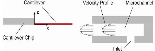
(5) Determination of the spring constants of the higher flexural modes of microcantilever sensors l. M n ( x)   (u n ( x' )  u n ( x)) Fp ( x' )dx'.. (2). x. If the modal shapes are normalized according to equation (1) the total energy in the n-th mode is given by [17]:. 2. Un . l 1 M n ( x) 1 2 dx   n .  2 0 EI ( x) 2. (3). Therefore, the additional bending moment ΔMn(x) induces a frequency shift Δ(n2):. l. 2  ( n )  2 u n ( x) M n ( x)dx. (4). 0. provided M n  M n and hence un is not significantly changed by the external forces. Substituting the expression for ΔMn(x) from equation (2) into equation (4) gives frequency shifts that depend only on the modal shapes un(x) and the external forces Fp(x). The correct normalization of the modal shapes can therefore be obtained if the external forces Fp(x) and the corresponding frequency shifts Δ(n2) are known.. In our experiments the external forces are caused by a fluid flow from a microchannel, with the flow direction parallel to the long axis of the cantilever (see figure 2) [10, 11].. Figure 2. Schematic of the experimental setup. A Poiseuille flow profile is established in the microchannel which interacts with the cantilever near the exit.. To provide information about the interaction of the flow from the channel with the cantilever we performed finite element method simulations with the open-source, multi-physics software package of 4.

(6) Determination of the spring constants of the higher flexural modes of microcantilever sensors Elmer [29]. Meshes required in the simulations were created with Gmsh [30]. The mesh independence of the results was confirmed by further mesh refinement. The forces applied to the static cantilever by the fluid flow were directly extracted from the simulations. Based on these forces the resonance frequency shifts were predicted according to equation (4).. 3. Experimental details Experiments were performed with a commercial AFM Explorer system (ThermoMicroscopes, Sunnyvale, CA, USA). A homemade smooth parallel plate microchannel fixed on the sample stage of the AFM was positioned such that fluid flow from its exit interacted with the cantilever as illustrated in figure 2. In this work, a channel of height H=150 m and length L=4.5 mm was used. The channel was mounted on micro-positioners (MDE262M, Elliott Scientific, UK) and aligned such that the cantilever was level with the top of the channel and with its free end 100 m from the channel exit. Nitrogen gas was used as the working fluid due to its low cost, high purity and well known properties. Pressure differences, Δp, were applied to the microchannel to drive the flow, establishing stable Poiseuille velocity profiles [10]. The maximum pressure applied to the channel in our experiments was ~1.4 kPa causing a velocity value of nitrogen in the channel mid-line of about 50 m/s [11]. The highest Reynolds number for our setup did not exceed 500. In combination with the Knudsen number in the channel, which is about 0.0005, this Reynolds number corresponds to the laminar regime of incompressible flow [31]. To test the method several commercially available tipless rectangular silicon cantilevers: 90-350 m nominal length, 0.03-1.75 N/m nominal spring constant, Al backside coating, (R-A to R-F, Mikromasch) and two V-shaped silicon nitride cantilevers: 205 m nominal length, 0.06 N/m nominal spring constant, Au backside coating (V-D, SNL, Bruker) and 196 m nominal length, 0.12 N/m nominal spring constant, Au backside coating (V-B, Veeco) were investigated. ‘Nominal’ refers to the information provided by the manufacturers. All rectangular cantilevers had a nominal width of 35 ± 3 m, cantilever V-B had a nominal leg width of 41 ± 5 m and V-D had a nominal leg width of 20 ± 5 m. The plan view dimensions of all microcantilevers were determined with an Olympus optical microscope. In addition, electron microscope images were acquired for the V-shaped cantilevers to obtain accurate geometric data of their tip dimensions and position. Power spectral densities of thermal noise spectra were recorded with an external interface with an accessible frequency range of ~700 kHz (National Instruments, USB-6251) as a function of fluid velocity. Resonance frequency values, Q-factors, and peak areas for each mode were monitored during measurement with a homewritten LabVIEW™ routine by fitting Lorentzian curves to the resonance. 5.

(7) Determination of the spring constants of the higher flexural modes of microcantilever sensors peaks similar to the procedure described in Ref. [19]. All resonance frequencies were monitored simultaneously. The resonant frequency values are based on the average of 50 individual spectra.. 4. Results 4.1 Cantilever dimensions The plan view dimensions of the tested cantilevers are reported in table 1. The base width of V-B was found to be 201.4 ± 2.3 m and that of V-D was 203.5 ± 1.9 m. The opening angle between the legs at the free end of the V-shaped cantilevers was therefore 56.5 ± 0.70 for V-B and 53.0 ± 0.6⁰ for V-D. For V-B and V-D the length was taken perpendicular to the end of the chip, the leg width was taken parallel to the cantilever base.. Table 1. Dimensions of the cantilevers investigated, lnom is the nominal length, lexp and wexp are the cantilever dimensions as determined by optical microscopy. Experimental uncertainties were derived from the standard deviation of at least three measurements. Cantilever. lnom (m). lexp (m). wexp (m). R-A. 110 ± 5. 95.5 ± 2.7. 28.4 ± 0.4. R-B. 90 ± 5. 76.3 ± 2.3. 28.9 ± 0.4. R-C. 130 ± 5. 114.7 ± 3.1. 31.1 ± 0.4. R-D. 300 ± 5. 295.0 ± 3.6. 31.2 ± 0.3. R-E. 350 ± 5. 339.5 ± 3.9. 31.4 ± 0.3. R-F. 250 ± 5. 240.1 ± 3.5. 30.3 ± 0.2. V-B. 196 ± 5. 187.4 ± 0.4. 39.8 ± 0.4. V-D. 205 ± 5. 204.0 ± 2.1. 25.5 ± 1.0. Significant discrepancies from the manufacturer’s dimensions were found, particularly in relation to the width of all the rectangular cantilevers and the lengths of R-A, R-B and R-C. As can be seen in figure 3, all rectangular cantilevers had a reasonably rounded or picketed free end. The quoted cantilever lengths were taken to be at the extreme of the structure.. 6.

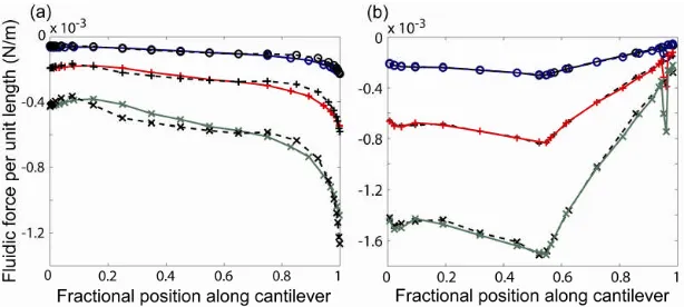
(8) Determination of the spring constants of the higher flexural modes of microcantilever sensors. Figure 3. Optical microscopy image of the plan view of cantilevers R-C, R-B and R-A (left to right of image).. 4.2 Forces exerted by the fluid flow Fluidic force distributions for a range of flow velocities were determined with Elmer for all cantilevers studied. Figure 4 (a) shows some of the forces per unit length exerted by the fluid flow along the cantilevers R-E and R-C at different fluid speeds as obtained from simulation. It was found that the force distributions for all rectangular cantilevers were remarkably similar for fixed fluid speed values if normalized to the cantilever length and hence a single force distribution (that of R-E) was used in the calculations of the spring constants. Figure 4 (b) displays the fluidic force for cantilever V-B with and without the tip. The influence of the tip is clearly visible as a sharp peak in the force at the tip position. There is only a very small deviation in the fluidic force at all other positions along the cantilever length.. Figure 4. Fluidic forces per unit length exerted by the flow of nitrogen from the microchannel depending on the fractional position along the cantilever length: (a) forces on cantilevers R-E (solid lines) and R-C (dashed lines) at fluid speeds of 6 (o), 15 (+), and 30 m/s (x), and (b) tipped V-B (solid lines) and tipless V-B (dashed lines) at fluid speeds of 6 (o), 15 (+), and 30 m/s (x).. 4.3 Frequency shifts. 7.

(9) Determination of the spring constants of the higher flexural modes of microcantilever sensors Theoretical frequency shifts fn2)=n2)/42 as a function of fluid velocity were determined according to equation (4) using the simulated forces with homewritten MATLAB routines, using modal shapes un(x) whose maximum deflection at the free end was set to one, i.e., with unnormalized modal shapes. Some of the results are displayed in figure 5.. Figure 5. Calculated frequency shifts (open circles) for the first four flexural modes of a rectangular cantilever. The predicted shifts are well described by a linear fit (solid lines).. Figure 6 shows experimentally obtained power spectral densities of the resonance peaks at zero fluid velocity for cantilever R-E together with the corresponding resonance frequencies and the Q-factors. The Q-factors of all resonant peaks showed fluctuations below 5-10% for different fluid speeds. Q-factors can therefore be considered as constant and independent of fluid velocity. This demonstrates that the frequency shifts observed at different fluid flow speeds are not due to a change of the dissipative forces in the z-direction of oscillation.. 8.

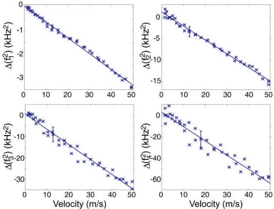
(10) Determination of the spring constants of the higher flexural modes of microcantilever sensors. Figure 6. Thermal noise power spectral densities of the first four flexural modes obtained for cantilever R-E.. Similar plots to those shown in figure 5 can be made with the experimental data. Figure 7 shows typical frequency shifts as a function of fluid velocity obtained experimentally for the first four modes of flexural vibration of cantilever R-E. The frequency shift fn2) decreases with mode number n as expected. This behavior was observed for all cantilevers investigated.. Figure 7. Experimental data (x) and fits (solid lines) of the frequency shifts as a function of fluid velocity for the first four flexural modes of cantilever R-E. Error bars are based on the experimentally 9.

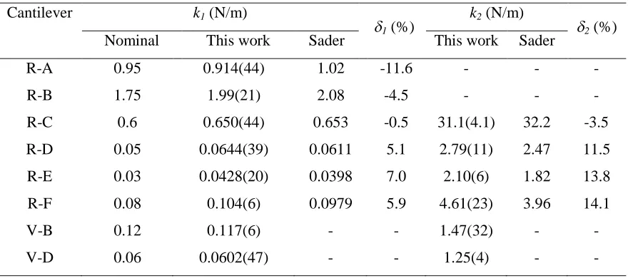
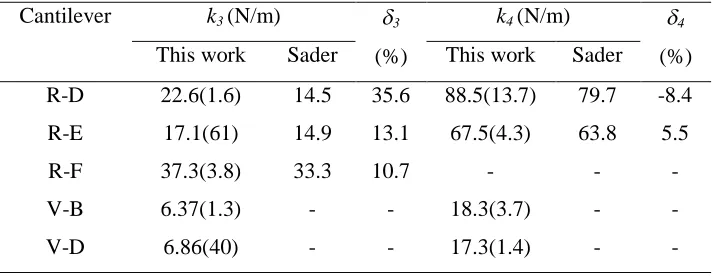
(11) Determination of the spring constants of the higher flexural modes of microcantilever sensors determined standard deviation of 15 measurements of the resonant frequency values at a constant fluid speed. Only one error bar for each mode is shown for clarity. The external moments M n (x) exerted by the fluidic forces are proportional to un(x). This allows for the determination of the normalization factor for un(x) (via equation (4)) by fitting a single parameter for each mode such that the calculated frequency shifts match those determined experimentally. The resulting normalized eigenmode shapes then comply with equation (1).. 4.4 Spring constants Spring constants of rectangular cantilevers were determined using both the method described above and the method of Sader [9] for all accessible flexural modes of oscillation. Values for the Sader method were determined using the experimental dimensions shown in table 1 along with the online calibrator for rectangular cantilevers [32]. Results are summarized in tables 2a and 2b. For some of the cantilevers presented here only the fundamental or first few modes were within the frequency range accessible with our equipment. The major source of uncertainty in our calibration comes from the fit of the experimental frequency shifts. Confidence bands based on one standard deviation were used in the calculation of the uncertainty. The resulting uncertainty in the spring constants is typically in the 5-10% range. Careful positioning of the cantilever eliminates the potential for related systematic errors in our calibration procedure. Table 2a. Spring constants for the first two modes of a variety of microcantilever sensors.  is the percentage difference between the spring constant derived by the method described in this work and that from the Sader method. The uncertainty in the last digits is given by the quantity in brackets. Cantilever. k1 (N/m) Nominal. This work. Sader. R-A. 0.95. 0.914(44). 1.02. R-B. 1.75. 1.99(21). R-C. 0.6. R-D. 1 (%). k2 (N/m). 2 (%). This work. Sader. -11.6. -. -. -. 2.08. -4.5. -. -. -. 0.650(44). 0.653. -0.5. 31.1(4.1). 32.2. -3.5. 0.05. 0.0644(39). 0.0611. 5.1. 2.79(11). 2.47. 11.5. R-E. 0.03. 0.0428(20). 0.0398. 7.0. 2.10(6). 1.82. 13.8. R-F. 0.08. 0.104(6). 0.0979. 5.9. 4.61(23). 3.96. 14.1. V-B. 0.12. 0.117(6). -. -. 1.47(32). -. -. V-D. 0.06. 0.0602(47). -. -. 1.25(4). -. -. 10.

(12) Determination of the spring constants of the higher flexural modes of microcantilever sensors Table 2b. Spring constants for modes 3 and 4 of a variety of microcantilever sensors.  is the percentage difference between the spring constant derived by the method described in this work and that from the Sader method. Cantilever. 3. k3 (N/m). 4. k4 (N/m). This work. Sader. (%). This work. Sader. (%). R-D. 22.6(1.6). 14.5. 35.6. 88.5(13.7). 79.7. -8.4. R-E. 17.1(61). 14.9. 13.1. 67.5(4.3). 63.8. 5.5. R-F. 37.3(3.8). 33.3. 10.7. -. -. -. V-B. 6.37(1.3). -. -. 18.3(3.7). -. -. V-D. 6.86(40). -. -. 17.3(1.4). -. -. Note that the relation between the static spring constant and the dynamic spring constants (measured for a force localized at the free end of the cantilever) is given by [28, 17]. k f ,static  ( n. 1 k f ,n. ) 1 ,. (5). where kf,static is the static spring constant, and kf,n is the dynamic spring constant of mode n. A value for the static spring constant can therefore be obtained based on the dynamic spring constant values.. 5. Discussion Our results based on both the simulation and the experiments indicate that forces and hence frequency shifts, fn2), depend largely linearly on the fluid speed (see figures 5 and 7). This can be explained by the fact that the force experienced by the cantilevers in our setup is essentially a drag force exerted by the fluid, which according to Stokes’ law increases linearly with speed [33].. 5.1 Cantilever positioning The positioning of the cantilever relative to the fluid flow is important although we found that in the current setup it is rather insensitive to deviations of several micrometers in the direction of the channel height and tens of micrometers in the distance from the exit.. 11.

(13) Determination of the spring constants of the higher flexural modes of microcantilever sensors If the cantilever was placed at the middle of the channel height, i.e. in the middle of the parabolic fluid velocity profile, however, we found a huge variation in the normalization factors extracted for the different individual modes. In consequence, there was also a significant deviation from the spring constant values reported in table 2a/b. We take the deviation in the normalization factors of the individual modes as an indication of a coupling of the flexural modes to the flow from the microchannel, with the strength of the coupling depending on the mode. It appears that the calculations we performed with a static cantilever do not describe this situation adequately and the steady-state approximation is no longer applicable. This is supported by studies of macroscopic flexible cantilevered plates positioned in the middle of a channel flow, see for example refs. [34, 35]. In the position that we used in our experiments the fluid flow can exert a force parallel to the cantilever length but the cantilever does not distort the main flow from the channel significantly because it is placed at the outer regions of the fluid stream. In fact, the cantilever can be considered to be an extension of the channel with flow essentially on one side only. The fluidic forces exerted normal to the cantilever length cause some static bending but do not change the oscillation frequencies if the bending is small and the cantilever behaves like an ideal beam [28]. The highest static bending observed occurred for R-E and was roughly 500 nm at the free end for the highest fluid speed of ~50 m/s based on the experiment. The theoretical calculation with the normal fluidic force distribution from the modeling gave a similar value [25, 17].. 5.2 Cantilever dimensions and shape All experimentally determined spring constants of the first flexural modes fall within the range given by the manufacturers, despite some of the dimensions of the cantilevers being outside the nominal range. The fundamental spring constants obtained for R-A, R-B, V-B and V-D are within the experimental error of the manufacturer’s nominal value. Generally, the fundamental spring constants calibrated using our method are in agreement with the values derived by the Sader method. No uncertainties are quoted for the Sader method but previous studies have found that an error of 15-20% is reasonable [36, 37]. For the higher modes (n>1) larger deviations are observed between the calibration methods. This is expected as the approximations made in the Sader method mean that it becomes progressively less accurate as the mode number increases [23, 38]. In other studies [36, 37] it has been found that the Sader method underestimates the spring constant due to a rounding-off of the free end or from a non-rectangular cross section of real cantilevers. Our results for R-D, R-E and R-F tend to support this, with the fundamental spring constants determined by our method being 5-7% higher than those determined by the Sader method. In addition, the Sader method requires that l>>w>>t, a condition that may not be totally satisfied by cantilevers R-A, R-B, and R-C which potentially explains why the Sader method appears to underestimate the spring constants for these cantilevers. The applicable lower limit of l/w is unclear, the minimum tested by Sader was l/w = 12.

(14) Determination of the spring constants of the higher flexural modes of microcantilever sensors 3.3, for which calibration by the Sader method showed reasonable agreement with other calibration methods [9]. It has also been noted that the errors associated with the Sader method increase with decreasing l/w [38]. Very close agreement between the two methods is evident for cantilever R-C. The deviations of the rectangular cantilevers from the ideal shape do not have a significant effect on our calibration procedure due to the small relative influence that it has on the fluidic force per unit length. All non-ideality in the cantilever dimension is effectively encoded in the modal shapes un(x), the experimentally determined normalization factors and the measured resonance frequencies of the cantilever. Only one set of theoretical frequency shifts was required in case of rectangular cantilevers if the simulated forces and mode shapes were normalized by the cantilever length. The deviation in the spring constants in comparison with using the correct force distributions (see figure 4) was below 6% for all rectangular cantilevers studied. The exact shape of the chip in the proximity of the fixed end of the cantilever was found not to be crucial. There was no significant difference in the overall resulting fluidic force and hence frequency shifts comparing a steep and a slanted chip wall. This can be explained by the fluid flowing mainly at the bottom side of the cantilever and the relatively small fluidic force at the fixed end due to the decreasing fluid speed with increasing distance from the channel exit (see figure 4).. 5.2.1 Influence of cantilever thickness. The thickness of a cantilever is crucial for its resulting stiffness [19], but it is in general much more difficult to determine it accurately than the plan view area dimensions. Calibration methods which do not rely on the exact knowledge of the cantilever thickness are therefore desirable. A 25% deviation of the cantilever thickness from its nominal value results in a factor of two difference in its flexural spring constant since it scales with the third power of the thickness [27]. Our modeling indicates that with the method presented here a 25% change in the thickness of the cantilever leads to a deviation of the determined spring constant value of less than ~3% compared to the correct value because of the small contribution of the cantilever side walls to the overall fluidic force. Therefore the exact cantilever thickness is much less crucial in obtaining accurate results here. In general the magnitude of the contribution depends of course on the thickness to width ratio but the error made by not knowing the thickness accurately will usually be small in our approach.. 5.3 Influence of tip It has been reported that the higher modal shapes can be significantly affected by the tip mass if it amounts to several percent of the total cantilever mass [13]. For the tipped V-shaped cantilevers studied the mass of the tip contributed less than 0.9 % to the total mass of V-D and less than 0.5% to the mass of V-B based on their dimensions obtained with electron microscopy. The determination of the modal 13.

(15) Determination of the spring constants of the higher flexural modes of microcantilever sensors shapes as described in ref. [17] indicated that there is no significant influence on the mode shapes compared to those of the same cantilevers without the tip, but it could be taken into account if required. The simulations further demonstrated that the effect of the tip on the fluidic forces experienced by the cantilevers is small. Figure 4 (b) shows the fluidic force per unit length for various speeds experienced by cantilever V-B with and without the tip. A pyramidal tip of 3.5 × 3.5 m2 at the base and 4 m in height was simulated based on the electron microscopy images. These dimensions appear to be typical for this type of cantilever in view of the manufacturer’s specifications. The presence of the tip has an influence on the fluidic forces, but it results only in a small increase of the magnitude of the frequency shifts fn2) of all modes. The increase was less than 3% for V-B and less than 1% in case of V-D. The effect on the change in the spring constants is therefore the same. For other types of cantilevers and tips there might be a bigger influence. To minimize the contribution from the tip to the fluidic force the setup could be changed such that the top of the cantilever is aligned with the bottom of the channel and the drag force is mainly exerted over the tipless top side of the cantilever. Note that with the normalized mode shapes, un(x), and resonant frequencies, n, known the spring constants for any force distribution and any tip position along the cantilever can be determined [17]. In particular any tip setback can be easily taken into account.. 5.4 Static spring constants. If static spring constants should be obtained based on the dynamic spring constant values then the error in the static spring constant will in general depend on the errors in the dynamic spring constant values and the number of dynamic spring constants known. For ideal rectangular cantilevers the difference between the static spring constant and the first dynamic spring constant is around 3% such that knowledge of the first few flexural spring constant values can already give quite accurate values [17]. The deviation between the static and the first flexural stiffness value however depends on the cantilever geometry in general and is around 10% for many V-shaped cantilevers [17]. Knowledge of several higher flexural stiffness values will give more accurate static spring constants but the error will depend on the number and accuracy of the higher stiffness values known and has to be determined for each case individually.. 6. Conclusions The spring constants of all flexural modes of microcantilever sensors can be calibrated with the method presented. In principle any cantilever could be calibrated using the approach described, provided the forces per unit length exerted on the static cantilever by the fluid flow, the unnormalized mode 14.

(16) Determination of the spring constants of the higher flexural modes of microcantilever sensors shapes un(x) and the eigenfrequencies n are known. Due to the use of a fluid flow the approach does not pose any risk of damaging the cantilever or the tip via contact with a surface. The technique does also not require accurate knowledge of the cantilever thickness, nor does it necessitate calibration of the cantilever deflection. The calibration can potentially be performed in any fluid−liquid or gas−and in low Q environments. The approach might therefore also prove to be useful in connection with the natural environments that are relevant in the life sciences and for biological systems in the future.. Acknowledgements Financial support from the University of St. Andrews is gratefully acknowledged.. 15.

(17) Determination of the spring constants of the higher flexural modes of microcantilever sensors References [1]. Giessibl F J 2003 Advances in atomic force microscopy Rev. Mod. Phys. 75 949-83. [2]. Parkin J D and Hähner G 2011 Mass determination and sensitivity based on resonance frequency changes of the higher flexural modes of cantilever sensors Rev. Sci. Instrum. 82 035108. [3]. Boisen A, Dohn S, Keller S S, Schmid S and Tenje M 2011 Cantilever-like micromechanical sensors Rep. Prog. Phys. 74 036101. [4]. McLoughlin N, Lee S L and Hähner G 2006 Simultaneous determination of density and viscosity of liquids based on resonance curves of uncalibrated microcantilevers Appl. Phys. Lett. 89 184106. [5]. McLoughlin N, Lee S L and Hähner G 2007 Temperature dependence of viscosity and density of viscous liquids determined from thermal noise spectra of uncalibrated atomic force microscope cantilevers Lab Chip 7 1057-61. [6]. Thomson N H, Fritz M, Radmacher M, Cleveland J P, Schmidt C F and Hansma P K 1996 Protein tracking and detection of protein motion using atomic force microscopy Biophys. J. 70 2421-31. [7]. Garcia R and Herruzo E T 2012 The emergence of multifrequency force microscopy Nat. Nanotechnol. 7 217-26. [8]. Sugimoto Y, Innami S, Abe M, Custance O and Morita S 2007 Dynamic force spectroscopy using cantilever higher flexural modes Appl. Phys. Lett. 91 093120. [9]. Sader J E, Chon J W M and Mulvaney P 1999 Calibration of rectangular atomic force microscope cantilevers Rev. Sci. Instrum. 70 3967-9. [10]. Lubarsky G V and Hähner G 2007 Calibration of the normal spring constant of microcantilevers in a parallel fluid flow Rev. Sci. Instrum. 78 095102. [11]. Lubarsky G V and Hähner G 2008 Hydrodynamic methods for calibrating the normal spring constant of microcantilevers Nanotechnology 19 325707. [12]. Lozano J R, Kiracofe D, Melcher J, Garcia R and Raman A 2010 Calibration of higher eigenmode spring constants of atomic force microscope cantilevers Nanotechnology 21 465502. [13]. Kiracofe D and Raman A 2010 On eigenmodes, stiffness, and sensitivity of atomic force microscope cantilevers in air versus liquids J. Appl. Phys. 107 033506. [14]. Senden T J and Ducker W A 1994 Experimental-determination of spring constants in atomicforce microscopy Langmuir 10 1003-4. [15]. Gibson C T, Watson G S and Myhra S 1996 Determination of the spring constants of probes for force microscopy/spectroscopy Nanotechnology 7 259-62. [16]. Holbery J D, Eden V L, Sarikaya M and Fisher R M 2000 Experimental determination of scanning probe microscope cantilever spring constants utilizing a nanoindentation apparatus Rev. Sci. Instrum. 71 3769-76 16.

(18) Determination of the spring constants of the higher flexural modes of microcantilever sensors [17]. Hähner G 2010 Dynamic spring constants for higher flexural modes of cantilever plates with applications to atomic force microscopy Ultramicroscopy 110 801-6. [18]. Neumeister J M and Ducker W A 1994 Lateral, Normal, and Longitudinal Spring Constants of Atomic-Force Mircroscopy Cantilevers Rev. Sci. Instrum. 65 2527-31. [19]. Hutter J L and Bechhoefer J 1993 Calibration of Atomic-Force Microscope Tips Rev. Sci. Instrum. 64 1868-73. [20]. Butt H J and Jaschke M 1995 Calculation of Thermal Noise in Atomic-Force Microscopy Nanotechnology 6 1-7. [21]. Stark R W, Drobek T and Heckl W M 2001 Thermomechanical noise of a free v-shaped cantilever for atomic-force microscopy Ultramicroscopy 86 207-15. [22]. Cleveland J P, Manne S, Bocek D and Hansma P K 1993 A nondestructive method for determining the spring constant of cantilevers for scanning force microscopy Rev. Sci. Instrum. 64 403-5. [23]. Sader J E 1998 Frequency response of cantilever beams immersed in viscous fluids with applications to the atomic force microscope J. Appl. Phys. 84 64-76. [24]. Sader J E, Larson I, Mulvaney P and White L R 1995 Method for the Calibration of AtomicForce Microscope Cantilevers Rev. Sci. Instrum. 66 3789-98. [25]. Hähner G 2008 Normal spring constants of cantilever plates for different load distributions and static deflection with applications to atomic force microscopy J. Appl. Phys. 104 084902. [26]. Timoshenko S, Young D H and Weaver Jr. W 1974 Vibration Problems in Engineering (New York: John Wiley ). [27]. Landau L D and Lifschitz E M 1991 Elastizitätstheorie (Berlin: Akademie Verlag). [28]. Courant R and Hilbert D 1968 Methoden der Mathematischen Physik vol 1 (Heidelberg: Springer Verlag ). [29]. http://www.csc.fi/elmer. [30]. Geuzaine C and Remacle J F 2009 Gmsh: A 3-D finite element mesh generator with built-in preand post-processing facilities Int. J. Numer. Methods Eng. 79 1309-31. [31]. Hetsroni G, Mosyak A, Pogrebnyak E and Yarin L P 2005 Fluid flow in micro-channels Int. J. Heat Mass Transfer 48 1982-98. [32]. http://www.ampc.ms.unimelb.edu.au/afm/calibration.html. [33]. Landau L D and Lifschitz E M 1991 Hydrodynamik (Berlin: Akademie Verlag). [34]. Balint T S and Lucey A D 2005 Instability of a cantilevered flexible plate in viscous channel flow J. Fluids Struct. 20 893-912. [35]. Howell R M, Lucey A D, Carpenter P W and Pitman M W 2009 Interaction between a cantilevered-free flexible plate and ideal flow J. Fluids Struct. 25 544-66 17.

(19) Determination of the spring constants of the higher flexural modes of microcantilever sensors [36]. Clifford C A and Seah M P 2005 The determination of atomic force microscope cantilever spring constants via dimensional methods for nanomechanical analysis Nanotechnology 16 1666-80. [37]. Kim M S, Choi J H, Kim J H and Park Y K 2010 Accurate determination of spring constant of atomic force microscope cantilevers and comparison with other methods Measurement 43 520-6. [38]. Chon J W M, Mulvaney P and Sader J E 2000 Experimental validation of theoretical models for the frequency response of atomic force microscope cantilever beams immersed in fluids J. Appl. Phys. 87 3978-88. 18.

(20)

No results found