Shape of transition layers in a differential–delay equation
Jonathan AD Wattis
School of Mathematical Sciences, University of Nottingham,
University Park, Nottingham, NG7 2RD, UK
April 19, 2017
Abstract
We use asymptotic techniques to describe the bifurcation from steady-state to a periodic solution in the singularly perturbed delayed logistic equation εx˙(t) =−x(t) +λf(x(t−1))withε ≪1. The solution has the form of plateaus of approximately unit width separated by narrow transition layers. The calculation of the period two solution is complicated by the presence of delay terms in the equation for the transition layers, which induces a phase shift that has to be calculated as part of the solution. High order asymptotic calculations enable both the shift and the shape of the layers to be determined analytically, and hence the period of the solution. We show numerically that the form of transition layers in the four-cycles is similar to that of the two-cycle, but that a three-cycle exhibits different behaviour. Asymptotic analysis, Differential–delay equation, transition layers
1
Introduction
The differential-delay equation (DDE)
εdx
dt =−x(t) +f(x(t−1)), (1.1) has been used by a variety of authors to model a wide range of physical phenomena, from population dynamics, as discussed by Gurney et al (1980), to physiology, where the production of red blood cells has been described by Mackey (1979); Mackey & Glass (1977); Glass & Mackey (1988) and Wazewska-Czysewska & Lasota (1976), to the behaviour of an optical cavity resonator, as studied by Ikeda (1979, 1985); Ikeda et al. (1980). In all these cases, the feedback function f(·)is nonlinear, having the form of a ‘humped’ function, that is, as x increases, f rises to a maximum and then decays. Variants of this system include a delayed logistic equation of the form dx/dt=λx(t)[1−x(t−1)], analysed by Fowler (1982), who used asymptotic methods to explain the periodic solution of large amplitude spikes separated by long small amplitude plateaus.
Equation (1.1) has been analysed using a range of mathematical techniques, for example, Erneux et
al. (2004) analyse the bifurcation to periodic solutions in the Ikeda system. Chow & Mallet-Paret (1983)
investigate chaotic behaviour in singularly perturbed differential-delay equations. Hale & Huang (1994) proved the existence of periodic orbits of (1.1) in certain parts of parameter space. The form of periodic solutions has been investigated by Chow et al. (1992) who note that asε →0, the waves become square, and have period approximately equal to two. Fowler & Mackey (2002) also note that the limitε ≪1 is singular, and use asymptotic analysis to describe the periodic solution in terms of relaxation oscillations.
Various properties about the form of the solution in the large time limit, and properties of the con-vergence to the square wave in the limit ε →0 have been rigorously established by Mallet-Paret and
1 INTRODUCTION 2
Nussbaum. Nussbaum (1982) proved the existence of slowly-oscillating periodic solutions. Bounds on their shape were established by Mallet-Paret & Nussbaum (1986), together with the fact that there may be multiple periodic solutions and multiple extrema in each period of oscillation. Mallet-Paret & Nuss-baum (1986) went on to prove that the period of the two cycle is 2+O(ε)and, by considering a coupled
problem for the two transition layer functions of the two-cycle, they establish bounds on the overshooting behaviour. They note that such behaviour is reminiscent of Gibbs phenomena in truncated Fourier series. The dependence of qualitative properties of the solution x(t) on the form of the nonlinearity f(·) was analysed by Mallet-Paret & Nussbaum (1989); in this paper they discuss how the solution profile approx-imates the square wave solution in the limit ε →0 for several example functions f(·). Mallet-Paret & Nussbaum (1993) consider the DDE (1.1) in the case where f(·)is a step function, and show that in this case solutions x(t)do not converge to solutions of xn+1= f(xn)in the limitε→0, but rather to a modified map. In contrast to this rigorous work, the approach taken here is to use asymptotic techniques to give simple explicit expressions for the shape of the transition layers.
Adhikari et al. (2008) also perform an asymptotic expansion of the waveform, obtaining an approx-imation in terms of elliptic functions and an expression for the period. Using global continuation of heteroclinic orbits, Chow et al. (1989) prove that transition layers in the periodic orbit are monotone, provided the nonlinearity f(x)is monotone. Fowler (1997) speculates that the onset of chaos is associated with a homoclinic connection of a periodic orbit in phase space.
These examples and analyses use a variety of nonlinear feedback functions, f(x); in this paper we focus on the simplest case, where f(x) =λx(1−x), which corresponds to the logistic map. This function is chosen for its mathematical simplicity, as it allows the period two cycle of the underlying difference equation to be explicitly determined.
In the limitε →0, the differential delay equation (1.1) reduces to the logistic map, whose properties we summarise in the remainder of this section. We also review the Hopf bifurcations in the DDE which occur for fixedλ asε >0 is reduced, and which lead to smooth periodic solutions. In section 2, we show that whenε=0 the solution x(t)has the form of a sequence of plateaus separated by discrete jumps. For 0<ε≪1, these plateaus are connected by narrow transition layers. Thus the bifurcation has quite distinct properties which the standard Hopf analysis fails to explain. It is the purpose of this paper to describe this bifurcation in more detail and, in particular, to analyse the form of these transition layers. In order to facilitate analysis of the transition layers, we introduce a reformulation of the problem, both for the general transition layer, and in particular for the two-cycle. In section 3 we construct asymptotic approximations to the solutions obtained when ε ≪1 and λ is increased through λ =3, which is the bifurcation point where the period two solution is created. Our analysis of this case shares some similarity with that of Adhikari et al. (2008); however, we avoid the use of elliptic functions. Section 4 contains a numerical investigation of the transition layers in the period 3 and period 4 cycles. In Section 5 we conclude the paper with a discussion of the key results.
1.1
Properties of the map
Whenε=0 the differential-delay equation (1.1) reduces to the logistic map
xn+1=λxn(1−xn), (1.2) which has been extensively studied, for example by May (1976) and Holton & May (1993). Here we summarise the results and properties of this map that are relevant to our later calculations, quoting the behaviour which is observed in each range ofλ values:
• for 0≤λ ≤1, there is only one fixed point in[0,1], namely x=0, and this is stable.
1 INTRODUCTION 3
• for 3<λ, the two fixed points x=0 and x=1−1/λ are both unstable. In this parameter regime, there is a two-cycle, given by
x±= 1
2λ
h
λ+1±p(λ−3)(λ+1)i. (1.3)
• for 3<λ ≤1+√6≈3.449 the two-cycle (1.3) is stable and is thus the attractor for the large n iterates. In this paper, we are predominantly interested in this range ofλ.
• for 1+√6<λ <3.544...the two fixed points and the two-cycle (1.3) are all unstable, and a four-cycle forms the stable long-time attractor.
• as λ increases further (λ >3.544), there is a succession of bifurcations to increasingly complex behaviour.
1.2
Hopf bifurcation
Chow & Mallet-Paret (1983) consider the differential–delay equation (1.1) and show that there is a Hopf bifurcation curve in (λ,ε)-parameter space. We reproduce these results here, partly for the sake of com-pleteness, but mainly to illustrate the qualitative difference between (i) the bifurcation and the form of solution obtained when one fixes λ >3 and reducesε, as Chow and Mallet-Paret consider, and, (ii) the case when 0<ε≪1 andλ increases through the valueλ =3, which we focus on in Section 3.
Here we make no specific assumptions on the values ofλ,ε, we treat them both asO(1)parameters.
We seek the region of parameter space where the uniform solution xs=1−1/λ is stable, by substituting
x=1−1/λ+δeγt+iωt into the governing equation (1.1) withγ,ω ∈Rand takingδ ≪1. AtO(δ)we
obtain
εγ+1=−(λ−2)e−γcosω, εω= (λ−2)e−γsinω. (1.4) This system of equations forγ,ω can be rearranged to give
tanω = −εω
1+εγ, (1+εγ)
2+ε2ω2= (λ
−2)2e−2γ. (1.5) A bifurcation occurs when the growth rate,γ, changes sign: the curve on whichγ =0 is given parametri-cally by
ε =−1
ω tanω, λ =2−secω. (1.6)
For smallε, solutions of the former equation can be approximated byω =nπ(1−ε+ε2)for any n∈N.
Substituting this approximation into the latter expression of (1.6) leads to a family of curves in (λ,ε) -parameter space which are approximated by
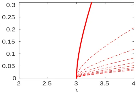
λn(ε) =3+12n2π2ε2, or εn(λ) = 1
nπ
p
2(λ−3), for odd n. (1.7) The first few curves are illustrated in Figure 1. The solid curve corresponds to the primary Hopf bifurca-tion, n=1; the curves corresponding to n=3,5, . . .yield solutions with higher frequencies.
As well as finding the location of the Hopf bifurcation in(λ,ε)parameter space, this method enables us to explicitly find an approximation for the solution, x(t). Fixingλ with 0<λ−3≪1, and reducingε so that only the primary (n=1) Hopf bifurcation curve is crossed, in (1.7), that is,
1 3π
p
2(λ−3) =ε3(λ)<ε<ε1(λ) =
1
π p
1 INTRODUCTION 4
λ
2 2.5 3 3.5 4
ǫ
0 0.05
[image:4.595.67.305.46.207.2]0.1 0.15 0.2 0.25 0.3
Figure 1: Illustration of the first few Hopf curves in(λ,ε)parameter space, as given by (1.6). To the left of the solid line, the steady-state is stable. The solid line represents the primary Hopf bifurcation curve. The dashed curves represent higher frequency instabilities which mean that when ε is arbitrarily small, the transition that occurs asλ increases fromλ <3 toλ >3 involves crossing many Hopf curves almost simultaneously.
results in a solution of the form
x(t)∼1−λ−1+αsin(πt(1−ε)), (1.9) withα ≪1. On the bifurcation curve, the period of the oscillation, P, is given by the frequencyω, which corresponds to n=1, namely
P= 2π
ω ∼2+2ε=2+
2
π p
2(λ−3), (1.10) withε≪1. Ifε is reduced further, so that several (1≤n≤J) other Hopf curves are crossed, that is,ε is given by
1
(2J+1)π
p
2(λ−3) =ε2J+1<ε<ε2J−1=
1
(2J−1)π
p
2(λ−3), (1.11) then a solution of the form
x(t) =1−1
λ +
J
∑
j=1
αjsin((2 j−1)πt(1−ε)), (1.12)
is obtained, which has the form of a truncated Fourier series. These series are known to be subject to Gibbs phenomenon, which is a term that describes the overshooting behaviour occurring when a discontinuous function is approximated by a Fourier series, for more details, see Gibbs (1898, 1899); Arfken (1985).
2 PRELIMINARIES 5
40 45 50
0.4 0.5 0.6 0.7 0.8
0 5 10
[image:5.595.57.438.41.190.2]0 0.2 0.4 0.6 0.8 1
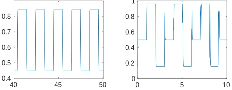
Figure 2: Illustration of a numerical solution of the DDE (1.1), for the caseλ =3.4 (left) andλ =3.8335 (right); in both cases,ε=0.01.
2
Preliminaries
2.1
General numerical results
Figure 2 shows a numerical solution, x(t), of (1.1) for two values of λ (produced using matlab solver dde23). The left panel shows a periodic solution with alternating high and low plateaus – a period 2 solution, which occurs when λ =3.4 and ε =0.01. There are sharp transition layers between the two plateaus, x− and x+ with x±given by (1.3), so that x+= f(x−)and x−= f(x+). Whenε =0, that is, for the one-dimensional map (1.2), this solution is stable for 3<λ <1+√6. When the solution of theDDE
(1.1) is considered withε>0, the period of the oscillation is greater than two.
The right-hand panel of Figure 2, illustrates the solution of (1.1) whenλ =3.8335, a value which corresponds to the stable 3-cycle of the one-dimensional map (1.2). In theDDE(1.1), the plateaus clearly follow the 3-cycle; however, in the DDE (1.1) the intervening transition layers do not show any form of periodicity, instead they become increasingly complicated, gaining both in their width and the number of oscillations. Thus the transition layers clearly show an instability. Our aim is to describe the initial stage of this development of complexity in the transition layers.
2.2
An approximate Poincar´e map
In order to describe and analyse the form of the transition layer, we rescale the time variable so that changes within the layers occur on an O(1) timescale. To achieve this, we write t = n+ετ, so that
εd/dt=d/dτ, and we describe each layer via a different functionψn(τ) =x(t), with n=0,1,2, . . .. Thus the DDE (1.1) can be rewritten as
ψn(τ) +
dψn(τ)
dτ =λψn−1(τ)(1−ψn−1(τ)). (2.1) We note that this transformation completely removesε from the problem.
The form ofψn(τ)is such that forτ=O(1),ψn(τ)describes the nthtransition layer. For large positive and negativeτ, with 1≪ |τ| ≪ε−1,ψn(τ)will be a constant, with potentially different constants at large positive and large negative values ofτ. For 1≪τ≪1/ε, we have
ψn(−τ)∼ψ−∞, ψn(τ)∼ψ+∞, with ψ+∞=λψ−∞(1−ψ−∞). (2.2)
We make a distinction between τ →∞ and 1≪τ ≪1/ε since τ =O(1/ε) corresponds to subsequent
2 PRELIMINARIES 6
corrections. At leading order, the matching conditions can then be written in the form
ψn(τ)→ψ−(n)∞, as τ→ −∞, and
ψn(τ)→ψ+(n)∞=λψ (n)
−∞(1−ψ
(n)
−∞) as τ→+∞. (2.3)
In addition, we haveψ+(n∞−1)=ψ−(n)∞andψ−(n+∞1)=ψ+(n)∞. The solution of (2.1) is
ψn(τ) =ψn(σ)eσ−τ+λe−τ
Z τ
σ e
sψ
n−1(s)[1−ψn−1(s)]ds, (2.4)
for arbitraryσ, which, in the limitσ→ −∞, leads to
ψn(τ) =λe−τ
Z τ
−∞e
sψ
n−1(s)[1−ψn−1(s)]ds :=F[ψn−1(τ)]. (2.5)
Due to its integral form, this version of the Poincar´e map may be useful for numerical simulations; however, our asymptotic analysis presented later will use the formulation (2.1). We will call the map
ψn=F[ψn−1]defined by (2.1) or (2.5) the ‘fast map’ since it describes the shape of the transition layers
which occur on the fast timescale. This has a similar form to a map used by Mallet-Paret & Nussbaum (1993).
2.3
Simulations of the 2-cycle’s transition layers
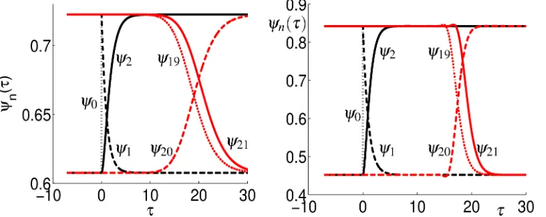
For 0<ε ≪1 and 3< λ <1+√6, we observe from numerical simulations of x(t), that there is a periodic solution, with period slightly larger than two. In figure 3 we illustrate the transition layersψn(τ) as calculated using (2.5), for n =0,1,2,19,20,21. This figure shows that successive applications of the map F on the discontinuous initial function ψ0(τ) =x−+ (x+−x−)H(τ), produces increasingly
smooth iterates. For large n the iterates are, modulo a phase shift, periodic with period two, that is
ψn+2(τ) =ψn(τ+2s)for some shift, which we write as 2s. Note that in the right-hand panel of Figure 3, for largerλ, the transition layers are not monotone, just before the descending layer starts its descent, it first increases and slightly exceeds the level of the plateau. Thus, in this parameter regime, the fast map (2.5) exhibits periodic behaviour with a period of two with a shift, s; that is
ψ2n(τ) → ψe(τ−2ns) as n→∞, (2.6) ψ2n+1(τ) → φe(τ−(2n+1)s) as n→∞. (2.7)
and our aim now is to find the form of the functionsψe,φe.
2.4
Instability of the fixed point of the fast map
The fast map (2.5) has a fixed point ψ(τ) =1−λ−1, which is the same as the fixed point of the one-dimensional map (1.2). To investigate the stability of the fixed point of the fast map, we introduce
ψn(τ) =1−λ−1+δζn(τ), (2.8) withδ ≪1 and linearising yields
ζn+1(τ) =L[ζn(τ)]:=−(λ−2)e−τ
Z τ
s=−∞e
sζ
n(s)ds. (2.9) Since this equation is a linear difference equation in n, it has solutions of the formζn(τ) =ρnζ(τ), where
2 PRELIMINARIES 7
Figure 3: Illustration of the iteratesψn(τ)plotted againstτ for n=0,1,2,19,20,21 for the case ofλ = 3.03 (left panel) and λ =3.4 (right panel). In both panels, ψ0 is the left-most dotted line, ψ1 is the
left dashed line, ψ2 is the left-most solid line, ψ19 is the right dotted line, ψ20 is the right dashed line, ψ21 is the right solid line. The curves corresponding to n=0,1,2 have transitions centred on 0<τ <5
(black curves, on the left side of the graph); whilst those with transitions around τ ≈20 correspond to
n=19,20,21, (red curves on the right). The online version is in colour.
instability occurs when |ρ|>1. The eigenvalues are given by ρ =−(λ−2)(1−iω)/(1+ω2), which
have magnitude|ρ|= (λ−2)/√1+ω2. Maximising|ρ|overω to find the first unstable mode, we obtain ω =0, corresponding toζ(τ) =1 andρ =−(λ−2). Thus, asλ increases through the value λc=3, ρ decreases through−1 and there is a period-doubling bifurcation.
After the bifurcation in the nonlinear equation (2.1), the derivative term is small and, to ensure it is involved in the leading order balance, we require∂τ =O(δ), hence we introduce a long timescale given
by T =δτ.
2.5
Two-cycle of the fast map
The period-two oscillation of the solution of the DDE corresponds to a two-cycle of the fast map, by which we mean that the second iterate of the fast map corresponds to a shift in the wave form, with no change in shape. That is, ψn+2(τ−2s) =ψn(τ)for some shift s, so that if, say,ψn(0) =1−1/λ then
ψn+2(2s) =1−1/λ, that is, the crossing of the unstable fixed point x=1−1/λ will occur at larger τ
when n is larger; equivalentlyψn+2(τ) =ψn(τ+2s)orF[F[ψ(τ)]] =ψ(τ+2s). From the numerics shown in Figure 3, we observe that
ψ2n(τ+2ns)→ψ(τ), ψ2n+1(τ+2ns+s)→φ(τ), as n→∞, for fixedτ. (2.10)
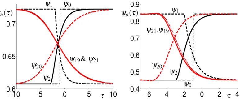
Estimating s=1, we obtain the results plotted in Figure 4. We observe that this leads to an almost com-plete cancellation of the shift:ψ21(τ+21)is close to being coincident withψ19(τ+19); however, there is
still some difference, hence s is not exactly unity. This estimate of s=1 in fact slightly overcompensates for the shift. In the following section, we use asymptotic techniques to extract a more accurate expres-sion for the shift, s, and obtain explicit approximations for the shape of the transition regions,ψ(τ)and
φ(τ) =F[ψ(τ−s)]. In particular, note that figure 4 shows that the transition layers are nonmonotone at
3 ASYMPTOTIC APPROXIMATION OF THE 2-CYCLE OF THE FAST MAP 8
Figure 4: Illustration of the iterates ψn(τ−n)plotted against τ for n=0,1,2,19,20,21 for the case of
λ =3.03 (left) andλ =3.4 (right). In both panels, the dotted square wave representsψ0, whilstψ1is the
steeper dashed curve containing a corner, andψ2 is the steeper solid curve;ψ19 is the other dotted line, ψ20, the other dashed curve, andψ21, the other solid curve, almost coincident withψ19. Note the different
scales on the horizontal axes. The transition layers for λ =3.03 are considerably more slowly varying than those forλ =3.4; also note that at largerλ, there is greater asymmetry in the shape of the transition layers. Left panel: the more slowly-varying curves correspond to n=19,20,21, whilst the steeper curves illustrate n=0,1,2. Right panel: the layers corresponding to n=0,1,2 are centred at −2<τ <0 are shown in red, whilst those for n=19,20,21 are centred onτ ≈ −3 and are shown in black. The online version is in colour.
3
Asymptotic approximation of the 2-cycle of the fast map
3.1
Problem formulation
Given the form of the two-cycle (1.3), we put
λ =3+δ2, (3.1)
and write the transition layers as
ψn(τ) =M+αΨn(τ), (3.2) where
M=λ+1
2λ =
4+δ2
6+2δ2, α=
p
(λ+1)(λ−3)
2λ =
δ√4+δ2
6+2δ2 , (3.3) so thatΨn→ ±1 or∓1 asτ→ ±∞. To be precise, we requireΨn(±∞) =±(−1)nso that if n is even then
Ψnis an ‘up’-layer (that is, increasing), and if n is odd, thenΨnis a ‘down’-layer, (decreasing).
Note that in this subsection, no assumption is made about the magnitude of δ. Only in the next subsection (§3.2) do we assume thatδis small. The effect of the fast map, which determines one transition layer as a function of the previous layer is given by
dΨn+1
dτ +Ψn+1+Ψn=
1
2δ(1−Ψ 2
n)
p
4+δ2. (3.4)
To analyse the two-cycle, with some phase shift s, we introduce
Ψ(τ) = lim
n→∞Ψ2n(τ+2ns), Φ(τ) =nlim→∞−Ψ2n+1(τ+2ns+s), (3.5)
3 ASYMPTOTIC APPROXIMATION OF THE 2-CYCLE OF THE FAST MAP 9
RequiringΨ2n+2to equalΨ2n modulo the phase shift, s, means that the shape of the transition layers
are governed by the coupled pair of differential–delay equations
Ψ(τ−s) +Ψ′(τ−s)−Φ(τ) = 12δ(1−Φ(τ)2)p4+δ2, (3.6) Φ(τ−s) +Φ′(τ−s)−Ψ(τ) = −12δ(1−Ψ(τ)2)p4+δ2, (3.7)
where the determination of s is part of the problem. Next we write
Ψ(τ) =ξ(τ) +ζ(τ), and Φ(τ) =ξ(τ)−ζ(τ), (3.8) so thatξ(τ) = 1
2(Φ(τ) +Ψ(τ))is the average shape of the transition layer, andζ(τ) = 1
2(Ψ(τ)−Φ(τ))
accounts for the asymmetry in the shape of the layers. The quantitiesξ(τ),ζ(τ)are governed by
ξ(τ−s) +ξ′(τ−s)−ξ(τ) = δξ(τ)ζ(τ)p4+δ2, (3.9) ζ(τ−s) +ζ′(τ−s) +ζ(τ) = 12δ(1−ξ(τ)2−ζ(τ)2)p4+δ2, (3.10)
together with the boundary conditionsξ(±∞) =±1 andζ(±∞) =0.
Thus far, we have not made any use of asymptotic approximations, beyond the fast map in Section 2.2, nor have we assumedΦ(τ) =Ψ(τ), orΦ(τ),Ψ(τ),ξ(τ)have odd symmetry, orζ(τ)is even.
3.2
Asymptotic expansion
We now make use of the approximation δ ≪1. Equation (3.10) implies ζ =O(δ), however, for the
simplicity of later calculations we introduce a slightly modified small parameter,ν, and write
ν= 12δp4+δ2, T =ντ, ξ(τ) =θ(T), ζ(τ) =νη(T), with θ,η=O(1). (3.11)
We note that the boundary conditions ξ(±∞) =±1 andζ(±∞) =0 imply
θ(T) → 1 as T →∞, θ(T) → −1 as T → −∞, (3.12)
η(T) → 0 as T → ±∞. (3.13)
Thus equations (3.9)–(3.10) imply
θ(T−νs) +νθ′(T−νs)−θ(T) = 2ν2θ(T)η(T), (3.14)
η(T−νs) +νη(T−νs) +η(T) = 1−θ(T)2−ν2η(T)2. (3.15) Note that if we just consider the leading order terms in (3.14), we obtainθ(T)−θ(T) =0. If we go to the next order terms, we find(1−s)θ′(T) =0, and sinceθ′=0 is not a possible solution, we require s=1, to leading order. However, this has still not generated an approximation forθ(T). To proceed further, we expand the delay s as
s=S0+νS1+ν2S2+O(ν3), (3.16)
where S0=1 has already been determined. We also write
θ(T) =θ0(T) +νθ1(T) +. . ., and η(T) =η0(T) +νη1(T) +. . . , (3.17)
3 ASYMPTOTIC APPROXIMATION OF THE 2-CYCLE OF THE FAST MAP 10
3.3
Leading order approximation of the 2-cycle
From the leading order terms in equation (3.15) it is clear that η0(T) = 12(1−θ0(T)2) and expanding
equation (3.14) toO(ν2)yields
ν(1−s)θ0′(T) +21ν2s(s−2)θ0′′(T) =ν2θ0(T)(1−θ0(T)2). (3.18)
Using (3.16) with S0=1 we obtain an autonomous problem forθ0, namely θ′′
0(T) +2S1θ0′(T) =−2θ0(T)(1−θ0(T)2). (3.19)
Multiplying through by θ0′(T)and integrating from T =−∞ to T = +∞ we find S1 R∞
−∞θ0′(T)2dT =0;
hence S1=0 (since the integral must be strictly positive). This is the secularity condition required by the
Fredholm alternative. TheODE(3.19) then simplifies and is solved byθ0=tanh(T). More generally, the
dynamics of this equation can be understood using phase planes; the system has a centre at (θ0,θ0′) = (0,0) and saddles at (θ0,θ0′) = (±1,0). The homoclinic trajectory joining the two saddles is given by
θ′
0=±(1−θ02)and corresponds to the transition layers, which are our main interest here.
Retracing our steps to find leading order approximations forΦ(T)andΨ(T)we recoverΨ(T),Φ(T) =
θ0(T)±νη0(T) and, since η0(T) = 21θ0′(T), the approximations for Ψ(T) andΦ(T) are simply phase
shifts of θ0(T). Furthermore, since s=1+O(ν2), we have also shown that the phase shift is unity to
leading order. In order to determine a more accurate approximation for the phase shift, we go to higher order in ν, where we will also find a correction term for the transition layer. This more accurate shape will explain the overshooting behaviour and asymmetry of the shape of the layers seen in Figures 3 and 4.
3.4
Higher-order terms
Substituting the expansions (3.17) into (3.14)–(3.15), and recalling that the delay term (3.16) simplifies to
s=1+ν2S2, we obtain the equations θ′′
0(T) =−4θ0(T)η0(T), 2η0(T) =1−θ0(T)2, η1(T) =−θ0(T)θ1(T), (3.20) 1
2θ1′′(T) +2η0(T)θ1(T) = 13θ0′′′(T)−2θ0(T)η1(T)−S2θ0′(T). (3.21)
Using the leading order solutionsθ0=tanh(T),η0= 12sech2(T)to simplify (3.21), we obtain θ′′
1 +2θ1(1−3 tanh2T) =2(1−tanh2T)(2 tanh2T−23−S2). (3.22)
As before, to find the correction to the phase shift, S2, we multiply through byθ0′ and integrate over T , to
obtain
S2=− Z ∞
−∞
2sech4(T)(2 tanh2(T)−23)dT
Z ∞
−∞
2sech4(T)dT =− 4
15. (3.23)
Thus, for 0<λ−3≪1 the shift per iterate of the fast map can be approximated by
s∼1−154ν2∼1−154δ2∼1−154(λ−3). (3.24) This explains why the unit shift applied between Figures 3 and 4 very slightly overcompensates for the shift.
Furthermore, the perturbation to the shape of the solution,θ1(T), can be calculated explicitly. The
complementary function for (3.22) has the form
3 ASYMPTOTIC APPROXIMATION OF THE 2-CYCLE OF THE FAST MAP 11
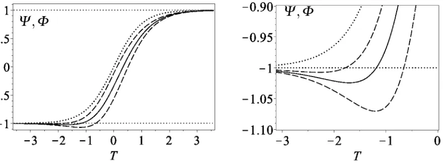
Figure 5: Illustration of the transition region functionsΨ,Φplotted against T including the first correc-tions to the tanh profile. The dotted lines represent Φ=Ψ=±1 andΦ=Ψ=tanh(T); the solid line shows tanh(T) +νθ1(T), which is nonmonotone, having values below -1 for T in the range for T<∼−1.18.
Here we have chosen a reasonably large value ofν, namely 0.46 to illustrate the behaviour. We also plot in dashed lines the functions tanh(T) +ν[θ1(T)±0.5sech2(T)], which include the effect ofη0=12sech2(T)
in (3.29) and (3.30). At smaller values ofν, this simply causes a phase shift in the profile, but this larger value of ν causes a more significant alteration to the shape. The right panel is a blow-up of the left, to show more clearly the effect of including the nonmonotonic, or ‘overshooting’ behaviour.
with A0,B0being arbitrary constants. A particular solution can be constructed by writing
θ1(T) =A(T)sech2(T) +B(T)u(T), (3.26)
and using the method of variation of parameters, which yields
A(T) = A0+45log(sech(T)) +101sech2(T)
1−13sech2(T) +3T tanh(T)sech2(T), (3.27)
B(T) = B0−101 tanh(T)sech4(T). (3.28)
Since the function u(T)∼e2T as T→∞, and we require boundary conditions in whichθ1→0 as T→ ±∞,
we choose B0=0. The combination B(T)u(T)then decays to zero as T→∞, with B(T)u(T)∼O(e−2T).
The constant A0is left arbitrary, as adding a small component, namelyνA0sech2(T), to the leading order θ0(T) =tanh(T) solution merely corresponds to a phase shift, namely θ0(T+νA0) =tanh(T+νA0).
Note that while A(T)grows linearly with T as T →∞, the combination A(T)sech2(T)is bounded. This product has the asymptotic decay ofθ1∼T e−2T as T →∞. The decay of this perturbation is thus slightly
slower than that of the leading order term, whose asymptotic behaviour is tanh(T)∼1−O(e−2T).
Inverting the transformations (3.8) to regainΨ,Φ, we find
Ψ(τ) = tanh(ντ) +1
2ν[2θ1(ντ) +sech
2(ντ)],
(3.29) Φ(τ) = tanh(ντ) +12ν[2θ1(ντ)−sech2(ντ)]. (3.30)
These functions are plotted in Figure 5. Since, for smallε, the two-cycle exists for 3≤λ ≤1+√6, the maximum relevant value forδ isδ =0.449, which yields a maximum value forν ofν =0.46, which is the value used in plotting Figure 5.
Relating our final time variable T back to the original variable t, we find
t−n=ετ= εT
ν = ε
T
4 TRANSITION LAYERS IN THE PERIOD 3 AND 4 CYCLES 12
-5 0 5
0.4 0.6 0.8
τ ψn
-5 0 5
0.4 0.6 0.8
τ ψn
-5 0 5
0.4 0.6 0.8
τ ψn
-5 0 5
0.4 0.6 0.8
[image:12.595.52.466.18.252.2]τ ψn
Figure 6: Illustration of the numerical solution of the fast map (2.1) whenλ =3.5, corresponding to the 4-cycle of the logistic map. Top left, iterates 1, 5, 9, 13; top right, iterates 2, 6, 10, 14; bottom left, iterates 3, 7, 11, 15; bottom right, iterates 4, 8, 12, 16; in each panel the iterates are denoted in the order ‘o’, ‘+’, ‘×’ and ‘2’; in each panel the third and fourth iterates appear identical.
We are interested in points in the transition layer, where T =O(1)and t−n is small. Since bothδ andε
are small parameters, and we expect the above expression to be small, we requireε≪δp1+δ2/4≪1.
In the next section we explore cycles with longer periods numerically.
4
Transition layers in the period 3 and 4 cycles
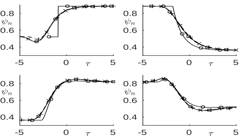
In Figure 6 we plot the transition layers for the four cycle as determined by a numerical solution of (2.1). In the logistic map the four-cycle is stable for 1+√6≈3.449<λ <3.544. Results are presented for the case λ =3.5 which is in the centre of this parameter range; the plateaus are given by x1=0.521,
x2 =0.884, x3=0.362, x4=0.819. We apply a numerically determined horizontal shift of s=0.9 to
the results to show the convergence in shape of transition layers at later iterates. Although six curves are plotted in each panel, most of those corresponding to later iterates cannot be seen as they lie on top of each other. The top left panel shows undershooting of the layer (ψ <x1) before converging to the
higher plateau, ψ =x2, whilst the layer plotted in the lower right panel exhibits both overshooting and
undershooting, that is, ψ >x4 and ψ <x1 for differing τ. Thus much of the behaviour discussed in
Sections 2.3, 2.5 and 3 persists in a qualitative fashion for the period four cycle.
5 CONCLUSIONS 13
0 5 10 15 20 25 0
0.5 1
τ ψn
0 5 10 15 20 25 0
0.5 1
τ ψn
0 5 10 15 20 25 0
0.5 1
τ ψn
-40 -30 -20 -10 0 0
0.5 1
τ ψn
-40 -30 -20 -10 0 0
0.5 1
τ ψn
-40 -30 -20 -10 0 0
0.5 1
[image:13.595.56.479.40.261.2]τ ψn
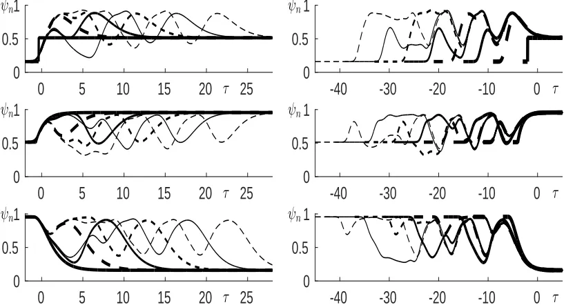
Figure 7: Illustration of the numerical solution for the fast map (2.1) whenλ =1+2√2, corresponding to the 3-cycle of the logistic map. On the left, a shift of s=0.35 is applied so that the left hand edges of the transition layers coincide. Top left, iterates 1, 4, 7, 10, 13, 16; middle left: iterates 2, 5, 8, 11, 14, 17; bottom left: iterates 3, 6, 9, 12, 15, 18; in each case, the order in which the iterates are plotted is given by solid thick line, dashed thick line, medium solid line, medium dashed line, thin solid line and thin dashed lines. In the right-hand panels, a shift of s=2 is applied so that the right edge of the transition layers coincide. Top right: iterates 1, 4, 7, 10, 13, 16, 19, 22; middle right: iterates 2, 5, 8, 11, 14, 17, 20, 23; lower right: iterates 3, 6, 9, 12, 15, 18, 21, 24; in each case the order in which the iterates are plotted is given by: very thick solid line, very thick dashed line, thick solid line, thick dashed line, medium solid line, medium dashed line, narrow solid line, narrow dashed line.
5
Conclusions
Any differential-delay equation of the form (1.1) which undergoes a bifurcation whereby the steady-state becomes unstable can be approximated by a quadratic. The analysis of the logistic map thus has a wider relevance to singularly perturbed differential-delay equations. We have studied such a differential-delay equation which, in the singular limit of smallε, reduces to the well-known one-dimensional logistic map. We have shown that as the 1D map undergoes a bifurcation to a period two state, so does the delay equation.
The analysis of Section 1.2 results in the formula (1.10) for the period of the oscillation on the bifur-cation curve. This formula only predicts the period of oscillation on the bifurbifur-cation curve (1.7), and is only valid for the case where harmonic solutions are produced, that is, away from the limit 0<ε≪1.
The solution of the singularly perturbed delay equation (1.1) has plateaus of approximately unit length, separated by narrow transition layers. In Section 3 we study the bifurcation which occurs asλ is increased through the value λ =3 withε ≪1. In this case, square wave solutions are produced, and the period depends on bothλ andε, and these parameters are treated independently in the result (5.1) which holds for more generalλ−3≪1,ε≪1.
By introducing the ‘fast map’, which is an approximate Poincar´e map, relating the form of each transition layer to the previous one, we have generated a further system of differential delay equations for the shape of the transition layers in the period-two cycle (3.7). In this system, the delay is an unknown parameter, for which we have generated an asymptotic expansion. The first few terms of this expansion are given in (3.24). In the original time variable (t) the period is
REFERENCES 14
This agrees with the result derived by Adhikari et al. (2008). For any particular choice of parameters, the period of the periodic solution depends on bothλ andε.
Analysing the fast map using asymptotic techniques, we have shown that, to leading order, the layers have a tanh shape, as might be expected. More significantly, in section 3.4 we have shown that the higher order perturbation terms give rise to more complex behaviour. In particular, the profile has an asymmetric shape, with nonmonotonic behaviour, and slower convergence to the plateaus than the leading order solution suggests. All these effects become more pronounced asλ increases beyond the bifurcation pointλ =3.
The form of the transition layers have been further explored through a numerical solution of the fast map in the cases of the four cycle and three cycle of the logistic map. In the four cycle, the transition layers again rapidly converge to one of the four steady shapes. Denoting the plateaus by x1,x2,x3,x4,
there are four attracting shapes for the transition layers, one for each of the x1−x2, x2−x3, x3−x4, and
x4−x1 layers illustrated in Figure 6. The transition layers between the three-cycle plateaus, however,
do not converge to a steady form. Instead, they grow in width, whilst showing some convergence in the shape of their right-hand edges. This increasing complexity provides considerable challenges for more theoretical analyses.
Acknowledgements
I am grateful to Andrew Fowler and Guy Kember for their advice during the preparation of my master’s thesis, Wattis (1990), and to the UK SERC for funding my studies. More recently, my thanks go to Louise Adams for performing preliminary numerical simulations. Helpful suggestions from referees have also improved the manuscript, including highlighting the papers by Nussbaum (1982), Mallet-Paret & Nussbaum (1993), and Adhikari et al. (2008) which contain some analysis similar to that presented here.
References
ADHIKARI, M.H., COUTSIAS, E.A., MCIVER, J.K. (2008) Periodic solutions of a singularly perturbed delay differential equation. Physica D 237, 3307–3321.
ARFKEN, G. (1985) Mathematical Methods for Physicists. Academic press, Orlando, Fl, USA
CHOW, S.N., HALE, J.K., & HUANG, W. (1992) From sine waves to square-waves in delay equations,
Proc. Roy. Soc. Edinburgh A 120, 223–229.
CHOW, S.N., LIN, X.B., & MALLET-PARET, J. (1989) Transition layers for singularly perturbed delay differential equations with monotone nonlinearities. J Dynamics and Differential Equations, 1, 3–43.
CHOW. S.N. & MALLET-PARET, J. (1983) Singularly perturbed delay-differential equations, in
’Cou-pled Nonlinear Oscillators.’ (ed. Chandra. J. & Scott, A.C.) North Holland Math. Studies 80 pp. 7-12.
ERNEUX, T., LARGER, L., LEE M.W., GOEDGEBUER, J-P (2004) Ikeda Hopf bifurcation revisited.
Physica D 194, 49–64.
FOWLER, A.C. (1997) Mathematical Models in the Applied Sciences. Cambridge, CUP.
FOWLER, A.C. (1982) An asymptotic analysis of the delayed logistic equation when the delay is large.
IMA J Appl Math. 28, 41–49.
REFERENCES 15
GIBBS, J.W. (1898) Fourier’s series. Nature, 59, 200.
GIBBS, J.W. (1899) Fourier’s series. Nature, 59, 606.
GLASS, L. & MACKEY, M.C. (1988) From Clocks to Chaos. Princeton University Press, (pp. 68–78).
GURNEY, W.S., BLYTHE, S.P., & NISBET, R.M. (1980) Nicholson’s blowflies revisited. Nature, 287, 17–21.
HALE, J.K. & HUANG, W. (1994) Period-doubling in singularly perturbed delay equations. J. Diff. Equ.
114, 1–23.
HOLTON, D. & MAY, R.M. (1993) Chaps 5–8 of MULLIN, T.,The Nature of Chaos, Oxford, OUP.
IKEDA, I. (1979) Multiple-valued stationary state and its instability of the transmitted light by a ring cavity system. Opt. Commun. 30, 257-261.
IKEDA, I. (1985) Delay-Differential Equations Modelling Nonlinear Optical Resonators, in ’Optical Instabilities’ (ed. Boyd, R.W. et al.) pp. 85-98.
IKEDA, I., DAIDO, H., & AKIMOTO, O. (1980) Optical turbulence: chaotic behaviour of transmitted light from a ring cavity. Phys. Rev. Lett., 45, 709-712.
MACKEY, M.C. (1979) Periodic auto-immune hemolytic anemia: an induced dynamical disease. Bull.
Math. Biol., 41, 829-834.
MACKEY, M.C. & GLASS, L. (1977) Oscillations and chaos in physiological control systems. Science
197, 287-289.
MALLET-PARET, J. & NUSSBAUM, R.D. (1986) Global continuation and complicated trajectories for periodic solutions of a differential-delay equation. Proc. Symp. Pure Math., Am. Math. Soc. 45 (pt.2), 155-167.
MALLET-PARET, J. & NUSSBAUM, R.D. (1986) Global continuation and asymptotic behaviour for
periodic solutions of a differential-delay equation. Ann. Mat. Pura ed Appli. 145, 33-128.
MALLET-PARET, J. & NUSSBAUM, R.D. (1989) A differential-delay equation arising in optics and
physiology. SIAM J. Math. Anal. 20, 249-292.
MALLET-PARET, J. & NUSSBAUM, R.D. (1993) Multiple transition layers in a singularly perturbed
differential-delay equation. Proc. Roy. Soc. Ed. 123A, 1119-1134.
MAY, R.M. (1976) Simple mathematical models with very complicated dynamics Nature 261, 459–467.
NIZETTE, M. (2003) Front dynamics in a delayed-feedback system with external forcing. Physica D
183 , 220-244.
NUSSBAUM, R.D. (1982). Asymptotic analysis of some functional differential equations. Pp. 277-302 of Bednarik, E and Cesari, L., Dynamical Systems II, an International Symposium, Academic Press, New York.
WAZEWSKA-CZYSEWSKA, M. & LASOTA, A. (1976) Mathematical Models of the Red Cell System.
Matemnatyka Stosowana, 6, 23-40.
WATTIS, J.A.D. (1990) Bifurcations and Chaos in a Differential-Delay Equation. MSc thesis, Univ of