The functional dendritic cell algorithm: a formal specification with Haskell

The Functional Dendritic Cell Algorithm: A Formal

Specification With Haskell

Julie Greensmith

University of Nottingham, Nottingham, UK, NG8 1BB

Email: [email protected]

Michael B. Gale

Abstract—The Dendritic Cell Algorithm (DCA) has been described in a number of different ways, sometimes resulting in incorrect implementations. We believe this is due to previous, imprecise attempts to describe the algorithm. The main contri-bution of this paper is to remove this imprecision through a new approach inspired by purely functional programming. We use new specification to implement the deterministic DCA in Haskell - the hDCA. This functional variant will also serve to introduce the DCA to a new audience within computer science. We hope that our functional specification will help improve the quality of future DCA related research and to help others understand further its algorithmic properties.

I. INTRODUCTION

Artifical Immune Systems (AIS) are an example of bio-inspired computing, where we focus on understanding the protective abilities of the human immune system and abstract these properties for a computational purpose. While some AIS focus on optimisation e.g. Clonal Selection based algorithms, a number of AIS concentrate on the detection of anomalies, often for computer security based applications. One such algorithm is the Dendritic Cell Algorithm [1]. It captures the behaviour of dendritic cells, whose responsibility in the immune system is to detect anomalies, to determine whether an immune response is required. Similarly, we wish to monitor information about computer systems in order to determine whether a response to unusual behaviour is required.

A key challenge thus far has been to find a clear specifi-cation of the DCA. The problem is twofold: firstly, explana-tions of the algorithm focus too heavily on the underlying biology and secondly, previous formal specifications have been imprecise and cluttered with implementation details. Imprecisions in previously published specifications are caused by the lack of explicit data flow, no types, and undefined functions. Different specifications of the algorithm have been presented for example in [1], [2], [3] and [4], which have led to some confusion in exactly the nature of the algorithm.

A better way to specify natural processes is offered by purely functional programming: the declarative nature of this paradigm allows to describe processes, rather than the imple-mentation of those processes. Additionally, the flow of data has to be made explicit. In other words, functions need to be pure in the mathematical sense: they cannot have side-effects such as the mutation of global state. This provides an elegant

platform for clear specifications of algorithms which can easily be translated into code. For example, the deterministic variant of the algorithm, the dDCA, can be defined as

dca = analyse◦process

to mean that the algorithm consists of a processing stage, followed by an analysis stage. This gives us a high-level overview of the algorithm, which we may then break down fur-ther by inspecting the definitions of theprocess andanalyse

functions. Our goal is to give a full specification of the DCA using this declarative style and to show how it can be applied in practice using the purely functional language, Haskell.

The main contribution of the paper is to present a definitive declarative specification of the algorithm and to show the validity of the functional haskell-based variant (hDCA). A secondary effect is to extend the interested audience for AIS by making the algorithm accessible to a different area of computer science by targetting an audience of functional programmers.

II. RELATEDWORK

A. The DCA: A History

The first DCA was presented in [5]. In this introductory paper a prototype of the DCA is presented, implemented in object oriented C++. The results of this study indicate that the algorithm is suitable for classification of preferably time ordered data. A full implementation of the algorithm was produced in [6] designed to work in soft realtime. This implementation is referred to as the ‘original DCA’. In related work, the first formal description of the algorithm is given in [2]. This system was refined and applied to the detection of port scans [1] and botnets [7].

was difficult to perform due to the large parameter set. This motivated the development of a deterministic variant (dDCA), so that a more concise and correct formal definition could be derived. The dDCA was presented in [3] as an evolution of the original DCA. However, it has a much reduced parameter set, resulting in a more controllable variant of the algorithm. This is the algorithm which we use to create the hDCA in this paper.

In 2010, [8] proposed FDCM, the fuzzy dendritic cell method. The two signal model is augmented and the FDCM employs fuzzy sets to transform the input stream data. This modification explores the boundaries of the cells decision variables. In their model this is translated into linguistic variables which are analysed using fuzzy subsets in place of the original method of using the signal transformation equation shown in [2]. Their experiments on real data have shown that an improvement in performance can be achieved using this method.

In his thesis, Gu [9] presented an extended version of the DCA (xDCA). This variant introduced automatic signal pre-selection and preprocessing, with antigen segmentation for large datasets. The data sources for the signal streams are automatically selected via feature selection mechanism, using principal component analysis (PCA). The hDCA as described in this paper uses a single invocation of the analysis process, however the xDCA includes dynamic invocation of the analysis component. The xDCA uses a dynamic time window of n events per analysis function invocation, or the analysis function is called every n seconds. The duration calculus is used to analyse the real time properties of the xDCA in this research.

B. Theoretical Research

A body of theoretical DCA research has emerged in par-allel with the evolution of the algorithm. The first formal description of the DCA was given in [2] and led to scrutiny of the algorithm. The first paper to analyse the algorithmics of the DCA is [10]. Filtering and noise reduction properties of the algorithm are exposed, and linear classifier properties suggested. Based on the filtering properties, the research is extended to study the DCA’s behaviour under uncertainty in [11]. A robust detection architecture is presented which may remedy some of the linear classification issues previously seen with the DCA.

The linear classifier aspects of the DCA are studied in detail in [12]. Models of the signal processing phase are constructed using the dot product, and the linear classifier properties are demonstrated. The results indicate that the DCA may suffer from the same problems as linear classifiers. This includes errors at classification boundaries and impaired performance for problems with complex or dynamic hyperplanes. These limitations are based on a variant of the DCA which does not require an antigen stream, and so only explores the signal processing aspect of the algorithm. Their conclusions are discouraging, that the DCA is not an effective classification technique and is not worthy of further research.

In response to the conclusions drawn in [12], [13] replaces the linear classification stage with a linear Support Vector Ma-chine. Both the modified and deterministic DCA is applied to a synthetic dataset alongside a standard linear classifier and a filtered linear classifier. The average performance of the DCA fell somewhere in-between the filtered and unfiltered linear classifier. The results also show that the DCA’s filtering prop-erties increase its performance when applied to noisy stream data, but shows poorer performance on traditional machine learning datasets. Their conclusions are also unfavourable and suggest that the DCA requires a training phase and additional classification components to increase its efficacy.

The limitation with the previously described studies is the lack of attention to the antigen or event stream and its influence on the final classifications. Muselle is the only author to have studied the influence of the event stream in the DCA [14]. In this work, a model of event stream behaviour is presented and validated using two synthetic datasets. A set of probability distributions are constructed. These distributions map to an alphabet of event types, generating different frequencies of event types. As the distributions are altered, the effect on the classification values is recorded. The study concludes that the DCA is robust to delays between stream data and motivated the use of streams in our fucntional specification, presented as the hDCA in the next section.

III. SPECIFICATION

Haskell is a purely functional programming language where the specification of a program is interpreted as its imple-mentation. It was chosen for the specification of the hDCA, being a popular functional language, and for its use of a type system which can reduce bugs in implementation. The hDCA specification consists of pure mathematical functions on sets, unlike in previous work, where the algorithm was presented using a sequence of abstract steps. We provide a concrete definition for each function from which an implementation can be derived. As a result, this specification is suitable for implementations in most programming languages, but can also be used to formally reason about the algorithm.

There are two parts to this specification. In the first part we describe set representations of objects used by the algorithm, such as cells and events. For an implementation, this part of the specification can be used to construct, for example, classes in object-oriented programming languages or algebraic data types in functional languages. The first part lays the foundation for the second part, where we describe the function definitions. This is achieved by defining the functions as mappings between sets from the first part.

that one signal represents “danger” and the other represents the “safe” signal. For example, when monitoring a server, “danger” may be associated with the amount of network traffic which is received while “safe” may be associated with low CPU usage [3].

The algorithm processes potentially infinite streams of input data, in an online style, which drive the iterative update of a circular queue of artificial dendritic cells. We refer to the number of iterations asn. In the original stochastic implemen-tation described in [6], the DCA is implemented as a real-time classifier used to analyse network data. When monitoring real-time data, n is the length of the monitored session, ensuring that results are analysed after n-many iterations. If the DCA is applied to a previously captured dataset,nis the size of the dataset. Reducing the value ofnfurther results in a technique termed antigen segmentation[1].

A. Preliminaries

In many embedded systems, such as network routers, there is not enough memory available to store large sets of data about, for example, network traffic [15]. At the same time, it would be desirable to process this data on a router. An elegant solution to this problem comes in the form of functional streams. A stream is just an infinite list. We define both structures inductively, beginning with lists. The set of lists over an arbitrary set X, denoted by ListX, is defined using

two cases:

1) The empty listε is an element ofListX.

2) If x ∈ X and xs∈ ListX, then x : xs ∈ ListX. We

readx:xsas “xconsxs”.

It follows that the empty wordεis an element of the set of lists over any setX. As long asX has at least one element,ListX

has an infinite number of elements. This is the case, because we can add each element inX to the start of any list inListX

using the second case. For example, suppose X ={1} then

1 :ε∈ListX, and 1 : (1 :ε)∈ListX and so on. For every

list x:xs, we refer to xas the head and xsas the tail. As a convention we name all variables using single lower-case characters, unless they represent lists in which case we name them using a lower-case character followed by ‘s’. We will adopt the same conventions for streams.

Since streams are lists which are always infinite, we can describe them inductively in the same way as lists, but with the case for the empty list removed. The set of streams over an arbitrary set X, denoted by StreamX, is therefore given

by:

1) If x∈X andxs∈StreamX, thenx / xs∈StreamX.

Here we also readx / xsas “xconsxs”. The different symbol is used so that we can distinguish between lists and streams more easily.

B. Inputs

There are two inputs to the hDCA, both of which are streams, based on the inputs defined for the dDCA implemen-tation. The first stream is referred to as the event or antigen stream. Events are elements of E×T, whereE is the set of

event types and T is the set of timestamps. The elements of Eare domain specific. In the port scanning example,Ecould be the set of port numbers, which would likely be represented by the set of natural numbers or, in an implementation, by unsigned 16-bit integers.

Timestamps are any total order with no upper bound which can be used to order inputs. For example, the natural numbers would be a suitable choice for T as we can tell that, for example, an event which took place at time 25 occurred before an event at time 26. We define the set of antigen streams as

A=Stream(E×T)

In the algorithm, we will have to inspect the timestamps of events. For convenience, we define a projection function which extracts the timestamp from an event:

tA : E×T→T tA(e, t) = t

The second input is referred to as the signal stream. This stream’s elements are members of T ×R1×. . .×Rλ. We define the set of signal streams as

S=Stream(T×R1×...×Rλ)

Similarly to the antigen stream, we will need to inspect the timestamps of signals. We define the following projection function for this purpose:

tS : T×R1×. . .×Rλ→T tS(t, . . .) = t

C. Cells

Dendritic cells receive input signals and use them to calcu-late threedecision signals: the activation signal, the inhibition signal, and the migratory signal. The process of calculating these signals is referred to as transduction. We represent the three signals using triples of real numbers:

Ω = R×R×R

Each dendritic cell consists of three components: a set of events; three signal values; and a migration threshold. The set of events is used as a buffer for the events which a cell encoun-ters during its lifetime. The signal values described above are also represented. The migration threshold determines a cell’s lifespan. We define the set of cell as:

Cell = P(E×T)×Ω×R

For convenience, we define a handful of ‘helper’ functions related to cells at this point. These allow us to give more concise and meaningful definitions later on. The first of these functions, new, initialises a new cell for a given migration threshold. The event buffer of the new cell is initially empty, while the decisions signals are set to 0.0:

new : _R→Cell

new(d) = (∅,(0.0,0.0,0.0), d)

function which evaluates to true if this has happened or false if not:

dead : Cell →B

dead(es,(ωA, ωI, ωM), d) = ωM ≥d

If dead evaluates to true for some cell, we may then use the reset function on the same cell to reset its event buffer and decision signals. The cell will keep its original migration threshold:

reset : Cell→Cell reset(es, os, d) = new(d)

We define a projection function calledeventsto obtain the set of events a dendritic cell has encountered during its lifetime:

events : Cell → P(E×T) events(es, os, d) = es

When a cell’s lifespan has reached its migration threshold, we wish to calculate aninterim anomaly scorefor the cell, which is then assigned to each event in the cell’s event buffer. There are two alternative methods which can be used to calculate the interim score. The boolean metric was referred to as the mature context antigen value (MCAV) in previous DCA literature, and the real metric referred to as Kα. This metric returns a probability of a particular event being classified as anomalous. We define it as follows:

score_B : Cell →_R

score_B(es,(ωA, ωI, ωM), ts) =

1.0 ωA> ωI

0.0 otherwise

If the activation signalωAis greater than the inhibitory signal ωI, then the cell classifies the events in its buffer as anomalous. The second anomaly metric used with the dDCA is the real metric, formerly known as theKαvalue. To calculate the real metric for a cell, we subtract ωI fromωA:

score_R : Cell→R

score_R(es,(ωA, ωI, ωM), ts) = ωA−ωI

The larger the number calculated by score_R, the greater likelihood that the events in the cell’s buffer are anomalous.

The algorithm maintains a population of cells, which is represented using an element of ListCell. Whenever a signal

is processed, the decision signals of all cells in the population will be updated and their lifespan will be increased. If an antigen is encountered, only the cell at the head of the population will be updated before it is put at the end of the list. This behaves somewhat like a circular queue in that we use a different cell for each event and loop back to first cell once the last has been used. We describe this process in more detail in section III-E. For now, we defineN to be the set of cell populations:

N = ListCell

We assume that there exists an initial population of cells initP op∈Nin which each element is constructed usingnew. The number of cells and their migration thresholds are the two key parameters in the dDCA and are tuneable. However, in all

implementations of the DCA, the number of cells present in the population at any one time is a constant number throughout the running of the algorithm. Previous research suggests that there is an optimum number of cells in terms of classification performance as shown in [16].

There can be a number of different approaches to selecting and setting the cells’ migration thresholds. As with the cell numbers, there is an optimum migration threshold range, though we do not know the exact function to determine this parameter value. Uniform, gaussian or random values have all been used previously to distribute migration threshold values throughout the cell population. A maximum migration thresh-old parameter is used to set the distribution. This maximum migration threshold is termed µ. Migration thresholds are examined in both [1] and in [4].

D. Output

Ultimately we are interested in obtaining a single anomaly score for each type of event the hDCA encounters. We represent the results using a set of pairs of event types and real numbers. For example, if the algorithm is monitoring processes in an operating system, a pair(4815,23.42) could mean that the process with ID 4815 has a normalised anomaly score of 23.42. We name the set of sets containing such pairsΘ:

Θ = P(E×R)

Intermediate results are members of a different setΦ. In this set, we pair up anomaly scores with events (as opposed to event types). We consider events to be instances of particular types of events. This allows us to distinguish between interim anomaly scores for the same event. It is possible that the same, interim anomaly score is calculated for the same event type more than once. If we would discard the timestamp of the event, we would end up with duplicate elements.

Φ = P((E×T)×R)

E. Algorithm

Now we have defined set representations for all data which is used by the algorithm. We proceed by describing the functions which form the hDCA. As described previously, the algorithm maintains a population of cells – an element ofN. Together with the two inputs, this forms the initial state of the algorithm. Since the functions in our specification are pure, we need to explicitly keep track of this state, using a structure which we term the hypervisor. For convenience, we give a name to the set of hypervisors:

H = A×S×N

From a high-level perspective, the algorithm is a function which maps a pair consisting of an event and a signal stream to a set containing an anomaly score for each event type:

dca : A×S →Θ dca = analyse◦run

“analyseafterrun”. The former of the two functions takes the two input streams as arguments and maps them to an element of the set of intermediate resultsΦ:

run : A×S→Φ

run(a, s) = process((a, s,initPop),0)

This function is primarily a wrapper for process which is given two arguments in addition to the two input streams: the initial population of dendritic cells initPop and an initial value for a counter. Since the input streams are infinite, we need to be able to decide when the algorithm should stop examining inputs and terminate. There are two key solutions: the first, which we will describe here, examinesn-many events and signals combined, where nis a pre-determined constant. The second examines infinitely-many items from both inputs, but yields results after every n-many iterations. In [17], time based segmentation is also used where n is substituted for a time based counter.

The behaviour of the first approach is implemented in the recursive process function. If the counter variablei is greater or equal than n, then terminate is called using the state of the hypervisor hto generate an element of Φ. This case ends the recursion. Otherwise, we perform one iteration using the

update function which will update the state of the hypervisor and may return intermediate results. The results are combined with those of a recursive call toprocess with the updated state and an incremented counter:

process : H×_N→Φ

process(h, i) =

terminate(h) i≥n φ∪process(h0, i+ 1) otherwise

where

(φ, h0) = update(h)

Once i is greater or equal to n, process is terminated. At this point, some cells in the population may still have events in their event buffers. In order to obtain anomaly scores for these events, we inspect the event buffers of all cells in the population and calculate interim scores for them interminate:

terminate : H→Φ

terminate(as, ss, cs) = {(e,score(c))|c∈cs, e∈events(c)}

An iteration of the algorithm leads to either an event update or a signal update. Theupdate function decides which of the two updates should be performed based on the timestamps of the first elements in both input streams. If the first event a has a timestamp lower than that of the first signals, an event update is performed. If the timestamp of s is lower or equal to that of a, then a signal update is invoked.

It is worth noting that the theoretical specification of streams shown in III-A can be implemented as shown if there is guaranteed to be no delay in accessing elements of both streams. In an implementation where elements in the streams are generated as data is received frome.g.a network, it may be desirable to extend the stream data structure with a flag which indicates whether data is available or not. The two timestamps may then only be compared if elements are at the heads of

both streams. Otherwise, it is safe to proceed with whichever stream has data in it or to wait if neither stream has available data.

update : H→Φ×H

update(a / as, s / ss, cs) =

(∅,(as, s / ss,updateA(a, cs))) tA(a)< tS(s) (r,(a / as, ss, cs00)) otherwise

where

cs0 = updateS(s, cs)

r = results(cs0)

cs00 = migrate(cs0)

Event updates result in an update of the population of dendritic cells. This is calculated by theupdateA function. It is given the event, an element ofE×T, which has triggered the update and the current cell population. We take the first cell in the population and extract its event bufferes, decision signalsos, and its migration thresholdts. The eventeis then added to the event buffer. Finally, we append the updated cell to the end of the list of cells in the population and return the updated population:

updateA : (E×T)×N →N

updateA(e,(es, d, t) :cs) = append(cs,({ e} ∪es, os, ls))

This function is the only part of the algorithm which changes the order of cells in the population. Since we always take the first cell for an event update and add it back to the end of the population, the cells are used in a circular fashion where we only use the same cell again after all other cells have also been used. Note that the definition ofappendhas been omitted as its definition is the usual, recursive one used by many functional programming languages.

Signal updates consist of three steps which are represented by the three equations in the where-clause in the definition of update: we begin by updating the decision signals of all cells in the population using the signal values obtained from the first element in the signal stream. This is done inupdateS.

Updating the decision signals results in an increased migratory value for each celli.eand increase inωM. As a result, we have to test for which cells this value has exceeded the respective migration threshold. Cells whose lifespan has exceeded their migration threshold generate intermediate anomaly scores for each event in their event buffer using the results function. We then reset these cells in migrate to generate an updated population.

Since we are working with signals, the following definitions change with the number of signals in the model. We give the definitions for the 2-signal model where λ= 2, but they can easily be extended for models with more signal categories by increasing the tuple sizes. The first step takes the form of a set comprehension in which we iterate through all cells in the old population and update their decision signals using the signal values:

updateS : (T×R1×R2)×N→N

updateS(( , s0, s1), p) =

The process of updating the decision signals is split into two functions: transduction maps the signal values to decision signals and accumulate adds those to the cell’s previous decision signals. The first of these two functions is an element of the following set:

transduction : (R,R)→Ω

In order to calculate the decision signals, a linear function is applied. We use formulas of the formω=w0∗s0+w1∗s0

whereωis the decision signal which is being calculated,sifor somei are the input signals, andwj for some j are weights. The following weights have been obtained from experiments with natural DCs:

ωA ωI ωM

s0 1.0 0.0 1.0 s1 −2.0 1.0 1.0

TABLE I

Results of a Paired Two Sided Wilcox Test comparing each population size against the default value for each event type, using the results across ten

sessions as the comparable data

The exact weights used in the algorithm do not change the behaviour, as long as the signs of the values are preserved. Inserting the weights from Table I leaves us with the following equations for the decision signals:

ωA = s0+ (−2.0)∗s1

ωI = s1

ωM = s0+s1

We use these equations for the definition of transduction:

transduction(s0, s1) = (s0+ (−2.0)∗s1, s1, s0+s1)

Once we have calculated values for the decision signals from the two input signals, we need to add them to a cell’s current values for the decision signals:

accumulate : Ω×Ω→Ω

accumulate((ωA, ωI, ωM),(ωA0 , ωI0, ω0M)) =

(ωA+ωA0 , ωI+ωI0, ωM +ωM0 )

The second and third step in the signal update are the same, regardless of how many signal categories there are. Each cell whose lifespan has exceeded the respective migration thresh-old is used to calculate an anomaly score for all the events in its event buffer. This is done using a set comprehension in the definition of results. This function is largely the same as theterminate function which we have defined previously, except for one difference: we only iterate through the events in a cell’s event buffer ifdead evaluates to true for that cell:

results : N →Φ

results(p) = {(e,score(c))|c∈p,dead(c), e∈events(c)}

Given the same population we have used as an argument for results and the helper functions which we have defined in section III-C, the process for resetting cells whose lifespan has exceeded their migration threshold is defined as follows:

migrate : N →N

migrate(cs) = {if dead(c)thenreset(c)

else c|c∈cs}

This set comprehension iterates through all cells in the population and tests if their migration threshold has been exceeded using dead. If dead succeeds, the cell is reset by reset which clears the cell’s event buffer and sets its decision signals to 0. The migration threshold of the cell is left untouched.

After n-many iterations, we stop processing inputs and return a set of events mapped to anomaly scores – an element ofΦ. This set is passed to theanalysefunction. At this point, we may have multiple interim anomaly scores for the same event type. Inanalysewe calculate the average anomaly score for each event type:

analyse : Φ→Θ

analyse(φ) = {(e, P

ν

|ν| )|e∈E}

where

ν={s|((e0_{, t), s)∈φ, e=e}0_}

Note thatν is calculated for each e∈E. In an implemen-tation, it may not be feasible to enumerate all event types if they are represented by, for example, 32-bit integers. Instead, it is possible to calculate a set of event types which are in use from φ by enumerating its elements. A suitable function for this purpose would be:

enumerate : Φ→ P(E) enumerate(φ) = {e|((e, t), s)∈φ}

The set returned byanalysecontains one anomaly score for each event type. For example, running the algorithm on a data set containing network traffic generated by different processes in a system may be produce a set such as:

{(bash,−108.15),(nmap,8.16),(pts,−23.4)(sshd,−42.0)}

IV. VALIDATIONEXPERIMENTS:DDCAVS HDCA

A. Domain Interfacing

The majority of traditional machine learning approaches rely on the classification of data points in n-dimensional hy-perspace. Such approaches use a feature vector representation for the dataset attributes. As we can see from the hDCA specification, the algorithm does not use feature vector input, but relies on the correlation between a set of signal streams and an event stream.

There are semantic differences between the kind of data mapped to the signal versus the event streams. The event stream contains events of specific types, which we wish to classify as normal or anomalous. In event log correlation the event stream is the capture of system calls from running processes. An event is represented as a process ID, each mapped as a single event type. The signal stream is composed ofcontextual datain which the event occurred. In applying the hDCA or indeed dDCA, the most crucial aspect is abstracting the signals as context information and not as direct attributes related to individual events. Ideal applications for the DCA are yet to be characterised, but experimental research shows that the algorithm can be applied to various two-class discrim-ination and correlation problems.

B. SCAN Dataset

Experiments in this section are performed on a dataset we term SCAN, first published in [2]. The problem is to detect if a host machine has been compromised and being used as a scanning relay. This is simulated through the running of an ICMP ping scan on a medium size network through a remote login. This scenario is used to create the dataset. This dataset consists of ten ICMP ping scans performed through a ssh remote login session using the network scanner, nmap [18]. A ping scan is chosen as it produces similar network reactions to scanning malware including scanning worms, but does not cause any damage to the network. Ping scans are extremely lightweight and so would also not denial of service the monitored network, yet would provide the essential changes in network behaviour to form an interesting dataset.

An event log is created containing the process ID for each system call invoked. A demon program is written to capture the network attributes. In this example we capture the rate of tcp packet sending and also record the rate of change of this variable using a moving average. Each scan session is between 45 and 60 sections in duration. A signal sampling rate of 1Hz is used. The frequency of event generation is variable, between 0 and 200Hz, depending on the process activity. Each dataset uses the same scenario protocol of “log in via ssh, initiate ping scan, wait for results, discover live hosts and logout”.

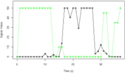
Data is generated for the signal streams by monitoring network attributes throughout the scenario. The signal stream contains two categories: a danger and a safe signal. These attributes are captured through the refresh of the data in the

proc filesystem contained within unix systems. The danger signal is derived from the rate of TCP packet sending. The raw

Fig. 1. A sample of the two signals varying over time during a single session. The grey line is the ‘safe signal’; the black line is the ‘danger’ signal.

values are scaled using min-max nomralisation within a range of 0 and 100. This in the SCAN dataset the danger signal operates at 1Hz and contains a real value of between 0 and 100 for every instance.

A good choice of safe signal is to have a real value which increases in proportion to the observation of normal behaviour in the monitored system. In the SCAN dataset, we use the burstiness or rate of change of tcp packet sending as a safe signal. This signal is also processed: min-max normalisation is used to transform the data into the range of 0 to 100. The normalised value is inverted so that the safe signal is zero when the burstiness level is high. Low burstiness is assumed to be an indicator of normal system behaviour, based on our expert knowledge of the problem domain. As a result we are left with two signal streams sampled at the same time and used as input to the dDCA and hDCA for this comparison.

To capture the data, demon programs are developed to listen to the outbound network traffic through capturing attributes of the tcp stream. Network data is captured from the proc filesystem. A graph of one of the datasets is shown in Figure1. We are interested in classifying four different event types in the SCAN dataset. Two of the event types are part of the port scan program. There are two anomalous event types, the nmap scan process and its parent the pts process. Two other normal event types feature in this dataset, the sshd process which manages the remote login and the bash process which controls the running of the opened remote shell.

C. DCA Implementations

Haskell is chosen as the implementation language for the hDCA used in these experiments. Given the declarative style of the specification, Haskell is the obvious choice. The code used is available from http://www.github.com/mbg/dca in literate Haskell. In terms of algorithm parameters, weights for signal categories are given in Table I. The maximum migration threshold is 100, as is the population size set to 100 as in [19].

1 2 3 4

−200

−150

−100

−50

0

50

100

Bash Sshd Nmap Pts

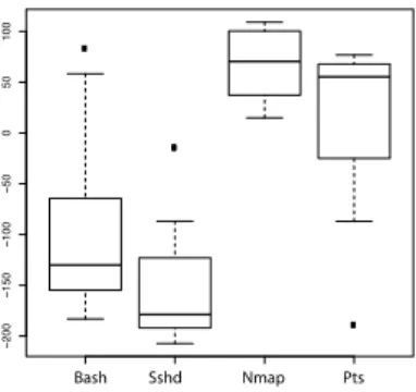
Fig. 2. Results using the real analysis method for the default setting of 100 cells with a maximum migration threshold of 100. Values are presented as medians across 10 port scan data sessions, shown for each event type. The nmap and pts are the anomalous processes, the bash and sshd are normal processes.

The results of applying the hDCA with the default parameters are shown in Figure 2. A clear discrimination between the normal and anomalous processes is shown.

V. CONCLUSIONS AND FUTURE WORK

Our main contribution in this paper is a novel and definitive specification of the dDCA inspired by functional program-ming. We used the declarative nature of the paradigm to specify the behaviour of the algorithm and avoided obscuring it with implementation details. We also focused on the inter-actions between different parts of the algorithm by showing how data flows through the algorithm. All functions in our specification are annotated with the sets to which inputs, outputs, and intermediate values belong to. Despite our choice to reduce implementation details, we were able to use the new specification to produce a working implementation in Haskell within minutes. We took our Haskell implementation and applied it to the previously used port-scanning to validate hDCA against dDCA. We hope that, together with the new specification, this will act as a guide for developers who wish to apply the DCA to problems in their respective domains.

Our new specification clearly distinguishes between differ-ent compondiffer-ents of the algorithm. [11] suggested that the analy-sis stage of the algorithm offers room to improve classification performance. Since our functions are pure, it is easy to replace them with different functions of the same type. This would allow us to modify the analysis function without having to change any other part of the algorithm. Indeed, once we have a new definition, we may use equational reasoning to prove properties about it with respect to the old definition.

Some details of our specification are designed to be simple, not computationally efficient. For example, the update func-tion traverses the cell populafunc-tion three times. This could likely be accomplished in just one traversal, which would be an easy (albeit not as neat) change to make. If we wish to use the hDCA in embedded systems such as network routers, analysis of the runtime performance will be required. This includes benchmarks as well as comparisons with other classification algorithms.

We hope that the use of purely functional programming to provide clear algorithmic specifications will inspire other algorithms in Natural Computing to be specified in the same way. We also believe that it will allow novel AIS to be described in a functional manner, thus making them more quickly accessible to a greater audience. Indeed, this would also simplify comparisons between different algorithms as we can use their specifications for equational reasoning, poten-tially providing a more theoretical grounding for future AIS.

REFERENCES

[1] J. Greensmith, “The dendritic cell algorithm,” Ph.D. dissertation, School of Computer Science, University Of Nottingham, 2007.

[2] J. Greensmith, U. Aickelin, and J. Twycross, “Articulation and clarifica-tion of the Dendritic Cell Algorithm,” inProc. of the 5th International Conference on Artificial Immune Systems (ICARIS), LNCS 4163, 2006, pp. 404–417.

[3] J. Greensmith and U. Aickelin, “The deterministic dendritic cell algo-rithm,” inArtificial Immune Systems. Springer, 2008, pp. 291–302. [4] F. Gu, J. Greensmith, and U. Aickelin, “Theoretical formulation and

analysis of the deterministic dendritic cell algorithm,”Biosystems, vol. 111, no. 2, pp. 127–135, 2013.

[5] J. Greensmith, U. Aickelin, and S. Cayzer, “Introducing Dendritic Cells as a novel immune-inspired algorithm for anomaly detection,” inProc. of the 4th International Conference on Artificial Immune Systems (ICARIS), LNCS 3627. Springer-Verlag, 2005, pp. 153–167.

[6] J. Greensmith, J. Twycross, and U. Aickelin, “Dendritic cells for anomaly detection,” in Proc. of the Congress on Evolutionary Com-putation (CEC), 2006, pp. 664–671.

[7] Y. Al-Hammadi, U. Aickelin, and J. Greensmith, “DCA for detecting bots,” into appear in Proc. of the Congress on Evolutionary Computa-tion (CEC), 2008, p. tba.

[8] Z. Chelly and Z. Elouedi, “Fdcm: A fuzzy dendritic cell method,” in

Artificial Immune Systems. Springer, 2010, pp. 102–115.

[9] F. Gu, “Theoretical and empirical extensions of the dendritic cell algorithm,” Ph.D. dissertation, University of Nottingham, 2011. [10] R. Oates, G. Kendall, and J. Garibaldi, “Frequency analysis for dendritic

cell population tuning: Decimating the dendritic cell.” Submitted to Evolutionary Intellegence, 2007.

[11] R. Oates, G. Kendall, and J. M. Garibaldi, “Classifying in the presence of uncertainty: A dca perspective,” inArtificial Immune Systems. Springer, 2010, pp. 75–87.

[12] T. Stibor, R. Oates, G. Kendall, and J. M. Garibaldi, “Geometrical insights into the dendritic cell algorithm,” in Proceedings of the 11th Annual conference on Genetic and evolutionary computation. ACM, 2009, pp. 1275–1282.

[13] F. Gu, J. Feyereisl, R. Oates, J. Reps, J. Greensmith, and U. Aickelin, “Quiet in class: classification, noise and the dendritic cell algorithm,” in

Artificial Immune Systems. Springer, 2011, pp. 173–186.

[14] C. J. Musselle, “Insights into the antigen sampling component of the dendritic cell algorithm,” inArtificial Immune Systems. Springer, 2010, pp. 88–101.

[15] A. Lall, V. Sekar, M. Ogihara, J. Xu, and H. Zhang, “Data streaming algorithms for estimating entropy of network traffic,” inProceedings of the Joint International Conference on Measurement and Modeling of Computer Systems, ser. SIGMETRICS ’06/Performance ’06, vol. Saint Malo, France, 2006, pp. 145–156.

[16] J. Greensmith, U. Aickelin, and G. Tedesco, “Information fusion for anomaly detection with the DCA,”Information Fusion, vol. 11, no. 1, pp. 21–34, 2010.

[17] J. Greensmith and U. Aickelin, “Dendritic cells for syn scan detection,” inProceedings of the Genetic and Evolutionary Computation Conference (GECCO 2007), 2007, pp. 49–56.

[18] F. Dostoevsky. (2013) nmap. last accessed, 5/10/07. [Online]. Available: http://www.insecure.org

[19] J. Greensmith, U. Aickelin, and J. Feyereisl, “The DCA-SOMe compari-son: A comparative study between two biologically-inspired algorithms,”