When does economic development promote mitigation and why?

Full Terms & Conditions of access and use can be found at

http://www.tandfonline.com/action/journalInformation?journalCode=tcpo20

Download by: [University of Nottingham] Date: 12 January 2017, At: 02:50

Climate Policy

ISSN: 1469-3062 (Print) 1752-7457 (Online) Journal homepage: http://www.tandfonline.com/loi/tcpo20

When does economic development promote

mitigation and why?

Zeynep Clulow

To cite this article: Zeynep Clulow (2016): When does economic development promote mitigation and why?, Climate Policy, DOI: 10.1080/14693062.2016.1268088

To link to this article: http://dx.doi.org/10.1080/14693062.2016.1268088

© 2016 The Author(s). Published by Informa UK Limited, trading as Taylor & Francis Group

Published online: 22 Dec 2016.

Submit your article to this journal

Article views: 155

View related articles

RESEARCH

When does economic development promote mitigation and why?

Zeynep Clulow

School of Politics and International Relations, University of Nottingham, Nottingham, UK

ABSTRACT

Is economic development compatible with mitigation? On the one hand, development should promote effective climate policy by enhancing states’ capacities for mitigation. On the other hand, economic growth creates more demand for production, thereby inhibiting emissions reduction. These arguments are often reconciled in the environmental Kuznets curve (EKC) thesis. According to this approach, development initially increases emissions in poor economies, but begins to lower emissions after a country has attained a certain level of development. The aim of this article is to determine empirically whether the EKC hypothesis seems plausible in light of emissions trends over the birth and implementation of the Kyoto Protocol. Drawing on data from the World Bank World Development Indicators and World Resources Institute Climate Data Explorer, it conducts a large-N investigation of the emissions behaviour of 120 countries from 1990 to 2012. While several quantitative studies have found that economic factors influence emissions activity, this article goes beyond existing research by employing a more sophisticated – multilevel – research design to determine whether economic development: (a) continues to be a significant driver once country-level clustering is accounted for and (b) has different effects on different countries. The results of this article indicate that, even after we account for country-level clustering and hold constant the other main putative drivers of emissions activity, economic development tends to inhibit emissions reduction. They also provide strong evidence that emissions trends resemble the EKC, with development significantly constraining emissions reduction in the South and promoting it in the North.

POLICY RELEVANCE

This article contributes to the understanding of the (changing) role of economic development in shaping emissions activity. It demonstrates the need for a contextualized, country-specific approach for evaluating the effectiveness of economic development in promoting emissions reduction and uncovers new evidence in support of the EKC hypothesis.

ARTICLE HISTORY Received 15 May 2016 Accepted 23 November 2016

KEYWORDS

Mitigation; environmental Kuznets curve; carbon trajectories; emissions and economic development

Introduction

Does economic development make countries more willing to protect the environment? Since the emergence of the sustainable development concept in the 1980s, economic development has frequently been heralded as the solution to environmental problems. Today, most policymakers worldwide in the Ministries of Energy, Economy and Environment believe that advanced economies have the ability to make more efficient use of natural resources, enabling them to limit the harmful consequences of economic activity on the environment. Yet this viewpoint is increasingly disputed, especially by structuralist scholars and policymakers in the geopolitical South. While accepting that economic development may enhance thephysicalcapacity for environmental pro-tection, proponents of this second approach assert that development also increases the demand for economic

© 2016 The Author(s). Published by Informa UK Limited, trading as Taylor & Francis Group

This is an Open Access article distributed under the terms of the Creative Commons Attribution License (http://creativecommons.org/licenses/by/4.0/), which permits unrestricted use, distribution, and reproduction in any medium, provided the original work is properly cited.

CONTACT Zeynep Clulow [email protected]; [email protected] School of Politics and International Relations, University of Nottingham, University Park, Nottingham, NG7 2RD, UK

activity, thereby placing more strain on the environment. In academic circles, both arguments often appear together in the environmental Kuznets curve (EKC) scholarship.1 According to this approach, development initially has an adverse effect on the environment, but then proceeds with lower and, eventually, negative environmental impact after a certain level of development has been attained.

These arguments are evident in debates surrounding the mitigation of the most challenging international environmental issue to date–climate change. On the one hand, economic development should promote effec-tive climate policy by enhancing states’capacities for emissions reduction (e.g. by increasing investment in carbon-efficient technology). On the other hand, economic growth inhibits emissions reduction by creating more demand for production. Many have reconciled these arguments by exploring the possibility that the development-emissions relationship resembles an EKC.2

The aim of this article is to determine empirically whether the effect of economic development on emissions trends resembles an EKC. Using data from the World Bank World Development Indicators, International Monet-ary Fund Export Diversification Database, United Nations Population Division, Freedom House Freedom Index and World Resources Institute Climate Data Explorer, it conducts a large-N investigation of the emissions trends of 120 countries from 1990 to 2012. Although several quantitative studies have found that economic factors influence emissions trends (e.g. Battig & Bernauer, 2009; Dolsak,2001; Lachapelle & Paterson, 2013; von Stein,2008), this article goes beyond existing research in two respects: First, it employs multilevel modelling to determine whether economic development continues to be a significant driver once country-level clustering is explicitly accounted for. Second, it develops a more sophisticated understanding about the influence of omic development on emissions activity by building a random coefficient model that allows the effects of econ-omic development to vary across countries.

The results of this article show that the influence of economic development on emissions activity is robust to country-level clustering: growth in per capita GDP tends to result in higher emissions levels. They also provide strong evidence that the influence of development on emissions trends varies markedly between different countries: the effect is strongly emissions-boosting in developing countries, but much weaker–and sometimes even inhibitory–in advanced economies. These seemingly contradictory findings lend support to the EKC hypoth-esis described above. Initially, until a certain level of socio-economic development has been attained, development severely increases emissions levels. Yet after a certain point, development transforms from inhibiting to promoting emissions reduction. Apparently, once governments have tackled pressing socio-economic concerns like poverty eradication, guaranteed the provision of basic human needs and invested in carbon-efficient technology, further bouts of development begin to reduce emissions, suggesting eventual compatibility with mitigation.

This article consists of four sections. The next section reviews the literature on international climate politics and the EKC to flesh out the main arguments that have been made regarding the influence of economic devel-opment on emissions activity. Section two outlines the research design by discussing the spatial-temporal domain, testing strategy and operationalization. The third section presents the results of the empirical analysis and runs a series of regional simulations to illustrate the likely effects of economic development on the key geo-political alliances in the multilateral climate negotiations. The article concludes by discussing the theoretical contributions and policy relevance of the findings.

Economic development and emissions trends

This section reviews the dominant arguments that have been made regarding the role of economic develop-ment in shaping emissions trends. It takes its cue from the EKC literature that contends that developdevelop-ment initially has a negative impact on the environment, but eventually becomes compatible with environmental pro-tection after a certain level of development has been attained. The EKC approach is compatible with the inter-national climate politics literature, which is drawn on in this section to map out the implications of the former body of work for emissions trends. This discussion provides the theoretical backbone for the central hypotheses tested in this article.

economic development, development increases the harmful effects of economic activity on the environment. Yet after a certain level of development has been attained,3further bouts of development begin to be associ-ated with lower environmental impacts.

There is a rich scholarship on the environmental effects of economic development more broadly. Most of this work falls beyond the empirical focus of this article–that is, the role of development in shaping emissions trends. The literature also identifies a range of indirect pathways whereby development interacts with other drivers (such as technology, demographics and emissions decoupling) to shape emissions. Although this discus-sion is clearly relevant to the topic of this article, the aim of this article is more modest: it is to investigate the independent effect of development on emissions trends while isolating other drivers. Therefore, indirect pro-cesses are not discussed here, but are used to inform critical decisions relating to model specification as set out in the research design section.

With these caveats in mind, the discussion now moves onto theorizing the direct effect of development on emission trends by focusing on three core pathways: industrialization, free trade and changing priorities. First, ceteris paribus, emissions levels tend to decline as a result of changes in the output mix which accompany the typical development path. In underdeveloped economies, specialization is on the production of unskilled, labour-intensive goods centred around agriculture (Betsill, Hochstetler, & Stevis,2006; Prum,2007; Roberts & Parks,2007,2008,2010). With economic development, specialization switches to heavy industries, changing the output mix and increasing emissions (Murthy,2016). In contrast, development in industrialized economies lowers emissions levels as production shifts to services and cleaner industries (Stern,2004).

Second, primary goods command lower prices in the world markets in comparison to skilled manufactures (Prebisch,1950), making exports from the former more accessible to advanced economies than the latter to developing countries.4 Free trade results in a transferral of high emissions activity to developing countries (Giljum,2004; Roberts & Parks,2010). Consequently, development in poor countries is more likely to be attained through the expansion of high carbon activity rather than transitioning to greener industries. Furthermore, the finite number of members of the world economy prevents latecomers to the development from outsourcing emissions to other parts of the world (Stern,2004).

Third, developing countries have scarce resources to divide between multiple goals and therefore channel these resources to more pressing, immediate concerns such as poverty eradication, the provision of clean drink-ing water, disease control and securdrink-ing basic livdrink-ing standards (Roberts & Parks,2007). In this socio-economic environment, the demand for development trumps environmental concerns – especially mitigation policy, whose benefits will only become apparent in the distant future (Gupta,1997; Prum,2007). Although economic development helps to alleviate these concern, eventually freeing-up resources for mitigation, the demand for further development and opportunity cost of emissions reduction continue to be extremely high. Thus as devel-oping countries develop and become more proficient in alleviating these concerns, development serves as a catalyst for more development, production and emissions. It is only after a certain level of development has been attained that mitigation begins to become a more politically, economically and socially viable priority.

In sum, these theoretical arguments generate two hypotheses that characterize the negative and positive parts of the EKC relationship postulated for emissions trends.

H1: At low levels of economic development, further bouts of development inhibit emissions reduction.

H2: At high levels of economic development, further bouts of development promote emissions reduction.

The remainder of this article evaluates these hypotheses empirically.

Research design

This article uses cross-section time series data to analyse the emissions trends of 120 countries from 1990 to 2012. The unit of analysis is the country-year, where one observation is the CO2 emissions level of a given

major negotiating alliances in the multilateral climate negotiations - namely: the EU, Umbrella Group (UG), BASICs, middle-income developing countries (MIDCs), LDCs and Alliance of Small Island States (LDCs and AOSIS),5OPEC and Central Asia, Caucasus, Albania and Moldova (CACAM).6The cross-sectional spread of the dataset reduces the risk that correlations are due to regional attributes rather than economic development.

The lower time limit was set to 1990 as this is the year that climate change entered the political agenda. Important developments in climate policy occurred over the following decades: countries convened to draft the UNFCCC in 1992, which was followed by the Kyoto Protocol (KP) in 1998. The race to bring the KP into force ushered in a dynamic period in climate diplomacy and widened transatlantic tensions, with the US with-drawing from the KP in 2005. In the seven years that followed, parties to the KP went on to achieve their col-lective emissions target over the First Commitment Period (FCP). If, as legal enthusiasts contend, international mitigation commitments do indeed have an impact on domestic emissions trends, then 2012 is an appropriate cut-off point as it marks the expiry of the KP, after which the climate regime entered a‘legal gap period’that is devoid of any binding targets. Presumably, then, the sudden expiry of mitigation commitments should have resulted in a laxer environment for emissions activity.7

Most quantitative work in the field employs ordinary least squares regression (OLS) (e.g. Battig & Bernauer,

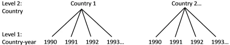
2009; Bernauer & Bohmelt,2013; Dolsak,2001; Lachapelle & Paterson,2013; von Stein,2008). Yet this article con-tends that the hierarchical structure of emissions trends violates the critical independence assumption that is implicit in single-level regression. For a variety of reasons–some of which are controlled for in this article– observations from the same country are more likely to be correlated than observations from different countries. Each observation of emissions trends is nested within a country, thus creating a two-level data structure as shown inFigure 1.

The veracity of this claim can be tested by conducting a likelihood ratio (LR) test on the emissions data to compare the two-level model described above with the equivalent single-level regression.8 Table 1shows the results of the null two-level model (excluding any predictors) and the LR test. Both of the variance com-ponents are significant at the 0.001 level. Regarding total variance in emissions levels, 91.4% occurs between countries, while the remaining 8.6% is attributable to longitudinal variation within countries. This is strong evi-dence that observations from the same country are correlated. Crucially, failure to account for clustering in the model could significantly underestimate the standard errors, resulting in erroneous inferences about the drivers of emissions trends.9Finding that economic development is robust to country-level clustering would provide strong evidence that it is an influential driver of emissions trends.

Figure 1.The hierarchical structure of emissions trends. Source: Word/PC.

Table 1.Results of the null two-level model.

Parameter Estimate

Fixed effects

Constant 159.41 (51.03)***

Random effects

Country variance 386,476.10 (44,959.00)***

Country-year variance 36,340.79 (898.47)***

LR test 7580.50***

Note: Coefficient entries are maximum likelihood estimates with estimated standard errors in parentheses. *Significant at 5% (p< 0.05).

Table 2provides an overview of the variables and data sources. Independent variables were centred in order to produce a stable succession of variance estimates across the models. EMTREND measures annual CO2

emis-sion levels in a country. The focus is on CO2levels because it is widely recognized as the worst offender and is

also the greenhouse gas for which the most comprehensive data are available. The dependent variable is

com-patibilitywith mitigation rather than mitigation per se. This is because the latter involves purposeful policies that

aim to promote emissions decoupling, whereas emissions trends (including reduction) can come about in the absence of purposeful policies (e.g. as a result of efficiency gains and technological changes).10Emissions data are taken from the World Resource InstituteClimate Data Explorer (CDE) database. Values range from near zero to 9312 MtCO2e, with higher scores denoting higher emissions.

Per capita GDP serves as a proxy for economic development. It provides a snapshot of average living standards, the cornerstone of socio-economic development, in a country in a given point in time. Arguably, then, per capita GDP is a better indicator of development than total GDP. Developed economies are associated with high per capita GDP levels. Per capita GDP data come from the World Bank WDI GDP figures for 1990 to 2012.

Since this article is primarily interested in the effect of economic development, the models hold constant the other (main) putative drivers of mitigation by including a series of control variables–namely: export diversity, annex status under the KP, share of national income derived from fossil fuels, renewable technology, population growth, emissions decoupling and democracy level.11Full details of the sources and coding strategy used to operationalize these variables can be found in the technicalappendix.

This article employs multilevel analysis to evaluate the influence of economic development on emissions trends.12It begins by setting up a single-level multivariate regression that incorporates all the variables from

Table 2. It then begins modelling the hierarchical data structure by setting up a random intercept model (RIM) which allows the intercepts to vary between countries. The final stage, the random coefficient model (RCM), also allows the effects of per capita GDP to vary between countries. Full details of the models and testing strategy are given in the technicalappendix.

Results

Table 3summarizes the results of the empirical analyses. The first set of interesting inferences are drawn from comparing the results of the single level and random intercept models, which are displayed in the first two columns. Crucially, as discussed above, the RIM coefficients are based on mean estimates across observations of emissions from the same country and thus indicate whether economic development effects are robust to country-level clustering. The RIM intercept indicates that the average country emits 78.4 MtCO2e per year.

After accounting for clustering and holding constant the other main putative drivers, increasing per capita GDP has a statistically significant, positive effect on emissions levels, suggesting that development is incompa-tible with mitigation. On average, a one-point increase in per capita GDP is associated with a 1.74 Mt increase in CO2emissions. Although the effect size is significant at the 0.05 level, it is only around a quarter of one standard

deviation of national emissions trends (651 points).

Would the results be any different if country-level clustering was unaccounted for? The OLS results in column one indicate that while economic development would continue to increase CO2 emissions levels,

Table 2.Variables.

Variable Definition Source

EMTREND Annual CO2emissions in a given country (MtCO2e) World Resource Institute Climate Data Explorer

GDP Per capita GDP (in US$ 1000s) World Bank World Development Indicators

EXPORTDIV Level of export diversification in the national economy International Monetary Fund Export Diversification Database

ANNEX Annex status in the climate regime Annex listings under the KP

FFDEP Ranked percentage of GDP dependent on fossil fuel income World Bank World Development Indicators TECH Annual proportion of renewable energy consumption as a

percentage of total national energy consumption

World Bank World Development Indicators

POP National population level United Nations Population Division database

EMDECOUP The ratio of change in CO2emissions to change in GDP World Resource Institute Climate Data Explorer and World Bank World Development Indicators

the effect would not be statistically significant. Although not the main focus in this article, the RIM indicates that the effects of most of the control variables are not robust to country-level clustering. In the flat regression, export diversification has a positive and significant effect on CO2 emissions. Yet this ceases to

be statistically significant in the RIM. Unexpectedly, emissions decoupling is associated with higher CO2

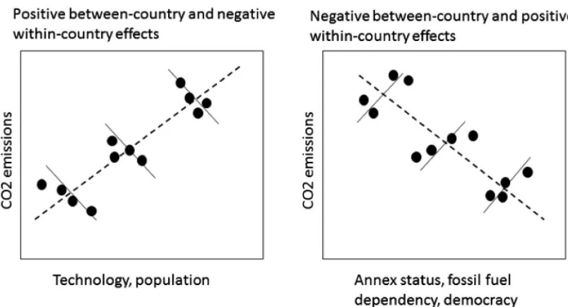
emis-sions in both models, although neither effect is statistically significant. Strikingly, the coefficients of all the other control variables undergo sign changes when country-level clustering is accounted for in the RIM. This important reversal in the direction of the effect of annex status, fossil fuel dependency, technology, popu-lation growth and democracy level points to the presence of cluster-confounding: these factors have contra-dictory effects on emissions trends within and between countries. Model 1 suggests that, on average, annex parties emit 24 MtCO2 emissions more than non-annex parties.13Yet model 2 suggests that a given country

is likely to emit 154 MtCO2more emissions when it is an annex party to the KP than it would otherwise emit

without annex status. From model 1, moving to a country with 1% higher reliance on fossil fuel incomes is (unexpectedly) associated with a 2.24 Mt decline in CO2 emissions. However, model 2 suggests that a 1%

increase in the fossil fuel dependency within the same country causes emissions to rise by 0.23 MtCO2.

Yet neither effect is statistically significant. The OLS suggests that, on average, CO2 emissions drop by

86.2 Mt with just one-point increase in the Freedom House democracy index.14Yet the RIM shows that, con-trary to widely held expectations, more democratic spells within the same country are associated with higher emissions, thus inhibiting mitigation.15Both the between and within-country effects of democracy are stat-istically significant. The remaining control variables suggest cluster-confounding in the opposite direction. The OLS shows that a country that derives 1% more of its total energy consumption derived from renewable technology tends to exhibit 2.49 MtCO2higher emissions. Yet in the RIM, technology has the expected

nega-tive effect on emissions: a 1% increase in the ratio of renewable energy consumption causes a 2.66 MtCO2

decline in emissions. Both technology effects are significant at the 0.001 level. Similarly, a country with a 1% higher population growth rate is associated with 0.25 MtCO2 higher emissions, although the effect is not

statistically significant. However, the RIM shows that a one-point increase in population growth rates within the same country is associated with a 2.25 MtCO2 decline in emissions, which is significant at the

0.01 level. A visual representation of the contradictory cross-sectional and longitudinal effects of these drivers is shown in the technical appendix.

Table 3.Compliance drivers.

Parameter Model 1 OLS Model 2 RIM Model 3 RCM

Fixed effects

Intercept 78.40 (27.04)*** 309.52 (66.64)*** 522.39 (228.51)*

Per capita GDP 1.09 (1.66) 1.74 (0.82)* 36.98 (20.52)

EXPORTDIV 1.81 (0.12)*** 0.06 (0.10) −0.01 (0.04)

ANNEX −0.24 (0.53) 1.54 (1.48) −1.00 (0.65)

FFDEP −2.24 (1.25) 0.23 (0.71) −0.18 (0.26)

TECH 2.49 (0.53)*** −2.66 (0.63)*** −1.00 (0.28)***

POP 0.25 (1.46) −2.25 (0.77)** −0.66 (0.26)*

EMDECOUP 0.35 (0.71) 0.03 (0.20) 0.03 (0.06)

DEM −8.62 (0.97)*** 1.77 (0.65)** 0.91 (0.23)***

Random effects

GDP random effect (u1) – – 49,078.55 (6805.53)***

Country variance – 467,883.90 (60773.70)***

R2:−21.06%

6185,963.00 (838,797.10)*** R2:−1500.60% Country-year variance 647.48 (9.57)***

Adj.R2: 12.03%

31,577.06 (959.65)*** R2: 13.11%

3048.95 (95.19)*** R2: 91.61%

LR testOLS – 5237.52*** 9803.31***

LR testNull – 15,574.62*** 20,140.41***

LR testRIM – – 4565.79***

Note: Single-level entries are ordinary least squares estimates and multilevel entries are maximum likelihood estimates with esti-mated standard errors in parentheses.

Modelling the random intercepts accounts for 13.1% of country-year level variance in the null model, only a small improvement from the 12% (adjusted) R-squared value in the single-level model.16Nonetheless, the LR tests confirm that the RIM performs significantly better than the equivalent OLS and null models.

Having established that economic development has a significant inhibitory effect on emissions reduction, the next step is to ascertain whether the effect is uniform. The third column inTable 3summarizes the results of the RCM with random country-level per capita GDP effects.

The first thing to report is the change in size and statistical significance of the per capita GDP coefficient. The fixed effect of per capita GDP increases substantially from 1.74 to 36.98, but ceases to be statistically significant in the new model. Crucially, this does not suggest that development is unimportant. In the RCM, the fixed effect estimate denotes theaverageeffect of per capita GDP when it is allowed to vary between countries. Yet, as illus-trated byFigure 3below, the average effect across all countries is a poor indicator of the typical effect of econ-omic development on emissions as the effect of per capita GDP varies significantly between countries.17Hence

thefixedeffect ceases to be statistically significant in the new model because the effect of per capita GDP varies

too much for the grand mean effect across all observations to be universally representative. Therefore, it would be wrong to generalize that economic development is strongly incompatible with mitigationin all countries. Moreover, the random effect term, u1, is highly significant at the 0.001 level, showing that per capita GDP is

indeed a significant driver of emissions trends, but has different effects on different countries.18The country-year level R-squared term and LR test result confirm that the RCM performs much better than the RIM and equiv-alent OLS.19Strikingly, the new model explains 91.61% of country-year variance, a significant improvement from the 13.1% R-squared value in the RIM.

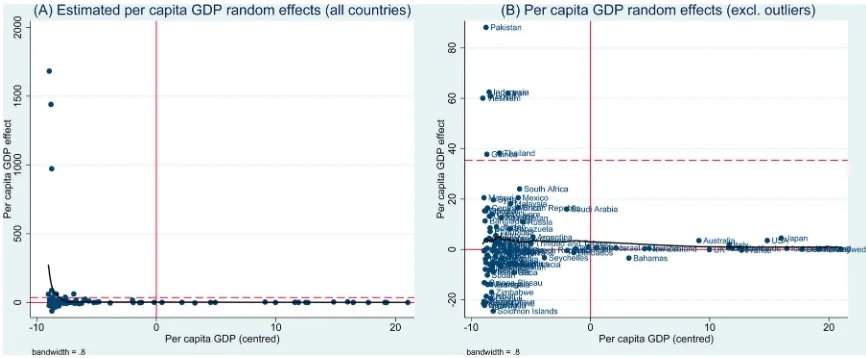
Having established that the influence of economic development on emissions trends varies significantly between countries, is it possible to say more about the nature of the heterogeneous effects?Figure 2plots the predicted country-specific (fixed plus random) effects of per capita GDP as a function of economic develop-ment (as indicated by per capita GDP). The dispersion of the country-specific effects around the fixed effect coef-ficient (represented by the horizontal dashed line) is striking. This is strong evidence that the fixed effect is a poor indicator of the role of economic development in shaping emissions.

Figure 2A plots the estimated effect of a one-point increase in per capita GDP (corresponding to US$ 1000) on each country’s CO2emissions. The dispersion of the points provides evidence of a mild negative relationship

between the effect and level of economic development. The graph starts off with a strong emissions-boosting effect at low levels of per capita GDP, and gradually weakens with economic development. The downward slope of the mean random effect line (random effects Lowess plot) indicates that economic development is associated with a decline in emissions-boosting effects on the y-axis. At high levels of economic development (on the right

Figure 2.Random country effects of per capita GDP on emissions trends. Source: Stata/PC.

of the x-axis), after US$ 15,000 beyond world average per capita GDP, further rises in per capita GDP exhibit negative effects on emissions, suggesting that development begins to become compatible with mitigation after this point.

The three points located in the top left quadrant ofFigure 3A exhibit exceptionally high random effects and may therefore skew the Lowess plot in favour of the negative relationship.Figure 2B checks for this possibility by plotting the same graph excluding the three outliers. The Lowess plot continues to slope downwards, showing that the negative relationship remains intact. Yet the gradient of the slope is much flatter at low levels of devel-opment where the outliers used to be, suggesting that improvements in per capita GDP are likely to drive up emissions levels by a significantly smaller amount than suggested inFigure 2A. On average, in the least devel-oped economies, a US$ 1000 increase in per capita GDP raises CO2emissions by 4 Mt, rendering it a moderate

impediment to mitigation in the poorest countries. Theoretically, then, the gradual decline in the emissions-raising effect of per capita GDP lends support to the EKC approach that economic development constrains climate policy until a certain level of development has been attained.

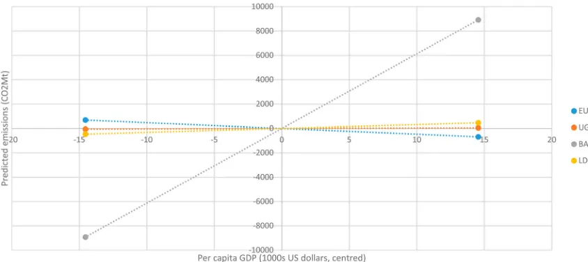
What do these findings tell us about the real world?Figure 3plots the mean posterior estimates of emissions trends of the four main bargaining blocks in the multilateral climate negotiations (namely: the Umbrella Group (UG), EU, BASICs and LDCs).20The lines represent the predicted economic development–emissions relationship for four hypothetical countries that possess the mean per capita GDP levels of each region across plus and minus one standard deviation per capita GDP. All other variables are set to zero, the grand mean across all observations on a centred scale, to isolate the independent effect of the predictor. Random intercepts were omitted to aid the visual comparison of the regional random effects from the same intercept.21

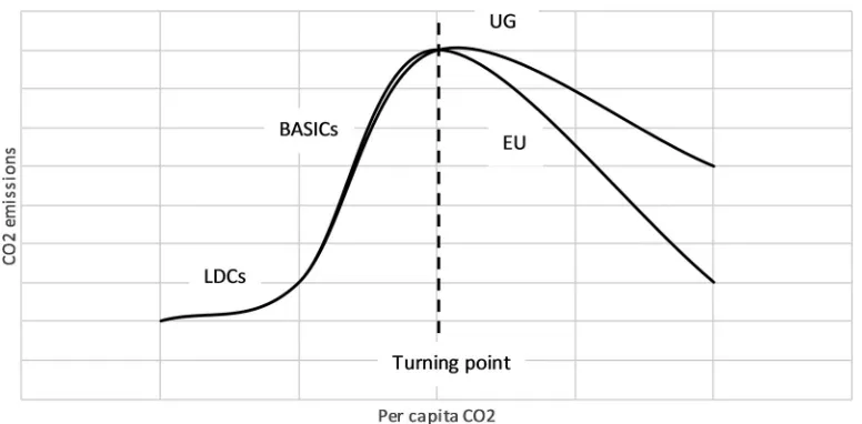
The angle and steepness of the line indicate the sign and magnitude of the effect respectively. Out of all four regions, the BASICs line exhibits the steepest slope, indicating that per capita GDP growth has the strongest emissions-raising effect in this region.22The LDCs line also follows a positive trajectory, indicating that develop-ment also drives up emissions in the poorest countries. Apparently, then, improvedevelop-ments in per capita GDP levels in the South are incompatible with mitigation, at least in the short-run. The flatter slope of the LDCs line relative to the BASICs slope suggests that the relationship is not linear as increases in per capita GDP do not result in parallel decreases in the emissions-raising effect of development. Instead, at least at low levels of per capita GDP, these predictions provide tentative evidence that the first part of the EKC is concave shaped–with the development effect starting out weak positive and becoming significantly stronger before flattening out at the turning point.23The proposed concave emissions-development relationship is depicted inFigure 4.

The regional simulations also provide some evidence of a turning point in the effect of per capital GDP growth on emissions. The flat slope of the UG line suggests that development is not an influential driver of emis-sions in the region. In other words, there has been a sharp reduction in the emisemis-sions-boosting effect of devel-opment, which, when combined with the high mean per capita GDP level of the region, locates the UG somewhere near the turning point inFigure 4. More interestingly, the negative slope of the EU line indicates that further bouts of development have the opposite effect of reducing emissions. The negative slope of the EU line suggests that the left-hand tail of the region’s EKC is sharper in comparison to the UG. Crucially, both regions are representative of the geopolitical North, in the sense that they have attained advanced levels of socio-economic development. Thus the findings of this article lend support to the popular claim that the relationship between economic development and emissions resembles an EKC. However, they do not explain why per capita GDP growth appears to have a stronger negative effect on emissions in the EU than the UG, suggesting the involvement of other factors (e.g. risk perception and energy lobbies).

While these results provide evidence of an EKC for emissions at the country level, emissions outsourcing cast doubt on whether these findings are likely to hold internationally. As various authors have pointed out (e.g. Pan, Phillips, & Chen,2009; Stern,2004; Stern, Common, & Barbier,1996), the transition to lighter industries such as services is usually accompanied by a rise in high-carbon imports. Although this does not negate the existence of an EKC-type relationship in the typical Northern country, it does suggest that the observed compatibility between development and mitigation in the North might come at the expense of increased incompatibility in the South. If the volume of emissions outsourcing continues to be high in the future, then, as latecomers to the economic development process, poorer countries are unlikely to be able to outsource carbon activity in the same way as their predecessors in the North, thereby locking them in the left side ofFigure 4.

Conclusion

The analyses presented in this article provide strong evidence that economic development is an influential driver of emissions trends. Even when country-level clustering is accounted for and the other leading putative drivers of emissions are held constant, per capita GDP was found to significantly affect national emissions levels. Most quantitative work in the field relies on fixed effect models, which estimate the average effect of develop-ment across all countries. The results of the RCM uncovered novel evidence that the effect of economic devel-opment on emissions varies significantly between countries. They also provided a more sophisticated insight

into the heterogeneous influence of economic development on emissions activity. At low levels of per capita GDP, economic development causes emissions to substantially increase. Yet the emissions-boosting effect of development gradually weakens as one moves to countries with relatively higher average per capita GDP levels, eventually reducing emissions. Both the positive sign of the fixed per capita GDP effect and gradual decline in the emissions-boosting effect of per capita GDP lend support to the EKC hypothesis that per capita GDP growth initially increases and then decreases environmental impact, suggesting that development eventually becomes compatible with mitigation.

The major policy implication of this research is that, at least in the short-run, economic development is likely to have the undesired effect of increasing emissions, making mitigation more difficult. The indications of this article are that this is likely to be happening in the most vulnerable regions which are still catching up with Northern living standards, especially in rapidly developing countries. Apparently, then, longstanding structural problems such as poverty eradication and dire living standards pose formidable obstacles to effective climate policy. This is probably compounded by emissions outsourcing from the North to the South. Thus further research needs to be done to identify the interrelated factors and processes that prevent the increased mitiga-tion capacity created by economic development from trickling down into emissions activity, particularly in the poorest parts of the world. Once these issues are addressed, conventional economic strategies designed to promote mitigation in the South should become significantly more effective. The good news is that economic development should begin to promote emissions reduction after developing countries have attained a certain level of economic development–so long as emissions outsourcing does not get in the way.

Notes

1. See, for example, Magnani (2001) and Stern (2004).

2. See, for example, Sengupta (1996), Dijkgraaf and Vollebergh (2001), Martinez-Zarzoso and Bengochea-Morancho (2004) and Galeotti, Lanza, and Pauli (2006).

3. This is sometimes referred to as the‘turning point’.

4. Dependency theorists refer to this as the‘declining terms of trade’. 5. Collectively, the LDCs and AOSIS comprise the most vulnerable states.

6. Country members of these groups can be found on the UNFCCC website:http://unfccc.int/parties_and_observers/parties/ negotiating_groups/items/2714.php.

7. As a robustness check, the models discussed below were also run on a smaller dataset spanning only the years in which Kyoto mitigation targets were active (i.e. over the FCP from 2008 to 2012) and showed no significant changes from the results obtained from the full dataset (from 1990 to 2012).

8. The LR value is the probability of obtaining the observed values (emissions data for the sample) if that model were true. 9. The risk of committing the type I error in single-level regression is well documented in the IR literature. See, for example, Jones

and Steenbergen (1997), Zorn (2001) and Bartels (2008). 10. Credit is due to two anonymous reviewers for pointing this out.

11. A series of lagged variables (t-1 to t-5) were initially included in the models to control for time dependency in emissions trends. Although the variables were statistically significant, the effect sizes were only small and, more importantly in the context of this research, did not significantly alter the coefficients of GDP or the control variables. Therefore, time series results are not reported in the results below.

12. All the models in this article were fitted using Stata’s xtmixed command.

13. The effect size of annex status is equal to 100 times the coefficient because ANNEX was multiplied by 100 to arrive at a com-parable range of values to the other independent variables.

14. Democracy scores were multiplied by ten during coding so the effect size is equal to ten times the DEM coefficient. 15. Battig and Bernauer (2009) find a similar effect and provide an in-depth discussion on why this might be.

16. The null model variance components were used to calculate the percentage of explained variance at each level of the model, which, according to Snijders and Bosker (1994), is the equivalent to having a separate R-squared value for each level of the multilevel model.

17. It is worth noting that, except for TECH and POP, all of the other control variables cease to be statistically significant once random per capita GDP effects are taken into account.

18. This is consistent with previous findings that development has heterogeneous effects on emissions across countries (e.g., Dijk-graaf & Vollebergh,2001and Martinez-Zarzoso & Bengochea-Morancho,2004).

20. Country members of these groups can be found on the UNFCCC website:http://unfccc.int/parties_and_observers/parties/ negotiating_groups/items/2714.php.

21. Consistent with the discussion above, the (absolute) sizes of the country intercepts are very large, which, when added to the estimated values in the figures, brings the emissions predictions within the expect range of values.

22. The regional simulations and negative slope of the Lowess lines inFigure 2give reason to expect that the steep BASICs line will gradually flatten and align with the other regional lines as the region meets its developmental needs.

23. Galeotti et al. (2006) report a similar finding.

24. To aid the interpretation of the democracy coefficient, the scores are inverted so that high (low) values denote high (low) levels of democracy.

25. Stata_’s unstructured covariance command was used to allow the random effects and intercepts to co-vary.

Disclosure statement

No potential conflict of interest was reported by the author.

Funding

This work was supported by the Economic and Social Research Council [grant number ES/J500100/1].

References

Bartels, B. (2008, July 9–11).Beyond‘fixed versus random effects’: A framework for improving substantive and statistical analysis of panel, time-series cross-sectional, and multilevel data.Paper presented at the Political Methodology Conference, Ann Arbor. Retrieved July 5, 2015, fromhttp://home.gwu.edu/,bartels/cluster.pdf

Battig, M., & Bernauer, T. (2009). National institutions and global public goods: Are democracies more cooperative in climate change policy?International Organization,63(2), 281–308.

Bernauer, T., & Bohmelt, T. (2013). National climate policies in international comparison: The climate change cooperation index.

Environmental Science and Policy,25, 196–206.

Betsill, M., Hochstetler, K., & Stevis, D. (Eds.). (2006).Palgrave advances in international environmental politics. Hampshire: Palgrave Macmillan.

Dijkgraaf, E., & Vollebergh, H. R. J. (2001).A note on testing for environmental Kuznets curves with panel data. Fondazinoe Eni enrico Mattei Working Paper N. 63.2001.

Dolsak, N. (2001). Mitigating global climate change: Why are some states more committed than others?Policy Studies Journal,29(3), 414–436.

Galeotti, M., Lanza, A., & Pauli, F. (2006). Reassessing the environmental Kuznets curve for CO2emissions: A robustness exercise.

Ecological Economics,57, 152–163.

Giljum, S. (2004). Trade, material flows and economic development in the south: The example of Chile.Journal of Industrial Ecology,8

(1–2), 241–261.

Gupta, J. (1997).The climate change convention and developing countries: From conflict to consensus?Dordrecht: Kluwer Academic. Jones, B., & Steenbergen, M. (1997, July 25).Modelling multilevel data structures. Paper presented at the 14th Annual Meeting of the

Political Methodology Society, Columbus, OH.

Lachapelle, E., & Paterson, M. (2013). Drivers of national climate policy.Climate Policy,13(5), 547–571.

Magnani, E. (2001). The environmental Kuznets curve: Development path or policy result?Environmental Modelling & Software,16, 157–165.

Martinez-Zarzoso, I., & Bengochea-Morancho, A. (2004). Pooled mean group estimation for an environmental Kuznets curve for CO2.

Economics Letters,82, 121–126.

Murthy, B. (2016). State of the environment in South Asia. In J. Raghbendra (Ed.),Routledge handbook of South Asian economics(pp. 289–308). New York: Routledge.

Pan, J., Phillips, J., & Chen, Y. (2009). China’s balance of emissions embodied in trade. In D. Helm & C. Hepburn (Eds.),The economics and politics of climate change(pp. 142–166). Oxford: Oxford University Press.

Prebisch, R. (1950).The economic development of Latin America and its principal problems.New York: United Nations.

Prum, V. (2007). Climate change and north–south divide: Between and within.Forum of International Development Studies,34(1), 223– 242.

Purdon, M. (2013). Neoclassical realism and international climate change politics: Moral imperative and political constraint in inter-national climate finance.Journal of International Relations and Development,2013, 1–38.

Roberts, T., & Parks, B. (2008). Inequality and the global climate regime: Breaking the north-south impasse.Cambridge Review of International Affairs,21(4), 621_–648.

Roberts, T., & Parks, B. (2010). Climate change, social theory and justice.Theory, Culture and Society,27(2_–3), 134_–166.

Roberts, T., Parks, C., & Vasquez, A. (2004). Who ratifies environmental treaties and why? Institutionalism, structuralism and partici-pation by 192 Nations in 22 Treaties.Global Environmental Politics,4(3), 22_–64.

Sengupta, R. (1996). CO2emission–income relationship: Policy approach for climate control.Pacific and Asian Journal of Energy,7, 207– 229.

Snijders, T., & Bosker, R. (1994). Modelled variance in two-level models.Sociological Methods and Research,22(3), 342_–363. von Stein, J. (2008). The international law and politics of climate change: Ratification of the United Nations framework convention and

the Kyoto Protocol.The Journal of Conflict Resolution,52(2), 243_–268.

Stern, D. (2004). The rise and fall of the environmental Kuznets curve.World Development,32(8), 1419_–1439.

Stern, D., Common, M., & Barbier, E. (1996). Economic growth and environmental degradation: The environmental Kuznets curve and sustainable development.World Development,24, 1151_–1160.

Sunstein, C. (2009).Worst case scenarios. Cambridge, MA: Harvard University Press.

Tuck, L., & Habib, B. (2014, July 9_–11).Climate change and relative gains in the wikileaks archive. Paper presented at the 6th Oceanic Conference on International Studies, Melbourne. Retrieved December 5, 2014, fromhttps://drbenjaminhabib.files.wordpress.com/ 2012/08/tuck-habib_ocis-2014_climate-change-and-relative-gains-in-the-wikileaks-archive.pdf

Vezirgiannidou, S. (2008). The Kyoto agreement and the pursuit of relative gains.Environmental Politics,17(1), 40_–57.

Technical Appendix

Control variables

As discussed in section two, Economic development and emission trends, most developing countries tend to be dependent on the export of unprocessed raw materials. Advanced economies, on the other hand, have the advantage of capital and know-how and thus tend to possess more diversified export sectors. (Betsill et al.,2006; Roberts & Parks,2007,2010; Roberts, Parks, & Vasquez,2004). EXPORTDIV is a continuous variable that measures a country’s reliance on the export of a few, barely processed raw materials, as a proportion of GDP. Data for export diversity come from the International Monetary Fund’s Export Diversification Index (EDI), which assigns countries a score from zero (low export diversity) to seven (high export diversity). ANNEX is a binary variable that is coded one for annex parties and zero for non-annex parties to the climate regime. Some argue that the lack of reciprocal quantitative targets for non-annex parties under the KP discourages annex parties from complying Kyoto emissions targets and, at least indirectly, inhibits mitigation policy (e.g. Purdon,2013; Tuck & Habib,2014; Vezirgiannidou,2008). Fossil fuel dependency (FFDEP) denotes the proportion of national income that comes from fossil fuels–either as an export or as a component of production. Countries with low dependency on fossil fuel incomes should comply more with the climate regime because they stand to gain from their ability to reduce emissions at a relatively lower opportunity cost than countries with high dependency (Sunstein,2009; Vezirgiannidou, 2008). Data for this variable come from the World Bank World Development Indicators (WDI) database records of the percentage of a country’s GDP that is accrued, in one way or another, from fossil fuels. Since this is (essentially) a neo-realist argument, which focuses on relative, as opposed to absolute, fossil fuel dependency levels, fossil fuel values from the WDI were centred for each year by subtracting the world mean fossil fuel dependency level in a given year from a country’s dependency score in that year. Democracies are regarded to be better at providing public environmental goods, therefore, they should comply more with Kyoto targets than non-democracies (Battig & Bernauer,2009; Bernauer & Bohmelt,2013). DEM is a discrete variable that is measured with the Freedom House political rights index. Countries are assigned separate scores from one (most democratic) to seven (least democratic) to denote the level of political rights and civil liberties.24_{Technology is expected to have positive effect on emissions}

reduction by improving efficiency in general (reducing the amount of input per unit of output) and purposefully reducing emissions per unit of output (Stern et al.,1996; Stern,2004). TECH models changes in emissions trends that are attributable to technology-induced efficiency gains by capturing the annual level of renewable energy consumption in a country as a percentage of final energy consumption based on data from the WDI database. POP uses data from the United Nations Population Division to measure annual demographic trends, which affect the demand for emissions activity. Sustainable development policy designed to reduce the environmental impact of economic activity should have a positive effect on attempts to reduce emissions irrespectively from the level of economic development. In accordance with the Organisation for Economic Co-operation and Development’s (OECD) authoritativeIndicators to Measure Decoupling of Environmental Pressure from Economic Growth(2005), this article operationalizes emissions decoupling by calculating the annual ratio of change in CO2emissions relative to change in GDP. Since decoupling seeks to divorce economic growth from emissions, EMDECOUP is only calculated for country-years with positive economic change values (i.e. economic growth). Scores are inverted to aid interpretation so that higher positive values denote more effective measures at decoupling than smaller positive values while negative scores indicate the very opposite of decoupling.

Testing strategy and models

Single-level model

EMTRENDij=b0+b1GDPij+b2EXPORTDIVij+b3ANNEXj+b4FFDEPij+b5TECHij

+b6POPij+b7DECOUPij+b8DEMij+eij.

(1)

The results of this model serve as reference for evaluating the insights of the two-level model described above.

Random intercept model

The next step is to check whether the effect of economic development that was identified in the OLS model is robust to country-level clustering. This is determined by examining the changes that occur in the signs, sizes and p-values of the coefficients once the same data is fed into the equivalent random intercept model (RIM):

EMTRENDij=b0+b1GDPij+b2EXPORTDIVij+b3ANNEXj+b4FFDEPij+b5TECHij

+b6POPij+b7DECOUPij+b8DEMij+uj+eij,

(2)

whereβ0is the overall mean compliance behaviour for all observations across all countries andβ0+ujis the mean compliance

Random coefficient model

The last stage in the analysis is to check for signs of heterogeneity in the effects of economic development by setting up a random coefficient model (RCM) which allows the slope of GDP to vary between countries:25

EMTRENDij=b0+b1GDPij+u1jGDPij+b2EXPORTDIVij+b3ANNEXj+b4FFDEPij+b5TECHij

+b6POPij+b7DECOUPij+b8DEMij+uj+eij. (3)

A significant random effect component (foru1jGDPij) would provide evidence of heterogeneous effects. The explanatory value

(equivalentR-squared values) of each model is evaluated by comparing the variance components with the null model results in Table 1and conducting LR tests between successive models.

Variables that exhibit cluster-confounding