Title:
Probabilistic analysis of a coal mine roadway including correlation control between model input parameters
Authors:
1. Andrew J Bootha– [email protected] (corresponding author) 2. Alec M Marshalla– [email protected]
3. Rod Stacea– [email protected]
aNottingham Centre for Geomechanics, Faculty of Engineering, The University Of Nottingham, University Park, Nottingham, NG7 2RD
Abstract:
Probabilistic analysis and numerical modelling techniques have been combined to analyse a deep coal mine roadway. Using the Monte Carlo method, a correlation control algorithm and a FLAC 2D finite difference model, a probability distribution of roof displacements has been calculated and compared to a set of measurements from an actual mine roadway. The importance of correlation between input parameters is also considered. The results show that the analysis performs relatively well, but does tend to over predict the magnitude of displacements. Correlation between parameters is shown to be very important, particularly between the three model stresses.
1. Introduction
There are two types of uncertainty; aleatory and epistemic [1]. In the context of geomechanics, aleatory uncertainty reflects underlying physical randomness and epistemic uncertainty a lack of knowledge about material and geometries [2,3]. Each must be treated differently; for example, it is possible to reduce epistemic uncertainty through field exploration or laboratory testing, in the sense that more information about a property reduces our uncertainty in it. However, more information will not reduce aleatory uncertainty [3]. This leads us to treating quantities in uncertainty analyses as random variables; that is, the quantity does not take a fixed value, but may assume any of a number of values, with it being impossible to know the true value until we observe it. Whitman [4] remarks that almost every factor dealt with in engineering analyses is truly a random variable, with some exhibiting more uncertainty than others.
Traditional design approaches are deterministic, where the lack of knowledge in the uncertainties is accounted for by introducing a factor of safety [5]. Analyses, sometimes referred to as reliability [5,6], probabilistic [7,8] or uncertainty [9,10], that try to account for the inherent variation in material properties, and other factors, are becoming more popular as the desire to assure satisfactory performance within the constraint of economy grows [5]. There are numerous approaches available, ranging in complexity and accuracy, to achieve these results, but what they all have in common is that they attempt to include the effects of property variability in a scientific way by using statistical methods [8].
In these approaches, all the model parameter inputs, whether they are, for example, dimensions, material properties, or stresses, are treated as random variables, expressed in the form of a probability density function (PDF). The aim of the exercise then becomes to estimate the PDF of some outcome, which is a function or dependent of the input random variables. It then becomes possible to give a probability to a certain value of the outcome occurring, such as the probability of failure, or more generally the probability of occurrence of an event.
One of the most widely used, and powerful, approaches to achieving this aim is the Monte Carlo method. First developed by researchers working on the development of the hydrogen bomb [11], the Monte Carlo method is now popular within fields ranging from finance to all manner of engineering. Baecher and Christian [2] divide Monte Carlo methods into two broad areas of use; firstly, the simulation of a process that is fundamentally stochastic, and secondly, problems that are not inherently stochastic but can be solved by simulation with random variables, such as the definite integration of a function. The work described in this paper falls into the first area.
Despite finding widespread popularity in many research topics of geomechanics, such as slope stability [13,21–24], tunnelling [25–27] and open pit mining [28–30], there are surprisingly few examples of its application to deep coal mining [10,31]. Brown [32] states that uncertainty analysis techniques, such as Monte Carlo, have found popularity in open pit mining over underground mining due to “the fact that the geomechanics risks associated with a given underground mining project or operation, including cases of deep and high stress mining, are likely to be more wide-ranging and varied than those associated with bench, inter-ramp and overall slope stability in a given open pit mine”. Canbulat [31] points to the difficulty in obtaining suitable and reliable distributions for the potentially many input parameters that can be required in an analysis of an underground mine. Some researchers have recognised the value of Monte Carlo analysis in the design and planning of deep coal mines, especially given that the need to assure economic viability of mining operations is at an all-time high. Lu et al. [10] and Canbulat [31] have both combined the Monte Carlo analysis with numerical methods to aid in the design and planning of roadways serving longwall panels in a coal mine. However, considering the significant variability encountered in deep coal mines, for example within material properties [31,33] and stresses [34,35], there is certainly scope for increased use and development.
Approaches often used to account for the variation in material properties include the single random variable (SRV) and random field [2,8,36]. Of the two approaches SRV is the simplest as the material properties are treated as random variables that do not vary across their region of definition [2], only between each model run. In the random field approach the spatial variation of material properties is taken into account through a spatial correlation structure, based on the spatial correlation length of the material property. The spatial correlation length parameter describes the distance over which material property values will be significantly correlated [21,23] and is currently not very well documented [13,21].
As part of work being conducted on an ongoing EU Research Fund for Coal and Steel (RFCS) project, a planning tool that will allow mining engineers to assess how much of a deep coal mine roadway may need additional work to ensure stability and operational requirements is being developed. As part of the same project, data regarding coal mine properties is being collected. This data was used in this work to obtain reliable probability distributions of input parameters, therefore addressing the issue raised by [31] and reducing the inherent epistemic uncertainty. The planning tool will use Monte Carlo analysis with the SRV approach for modelling the variability of material properties, in conjunction with numerical modelling, to provide a probability distribution of roof displacements. By using this distribution, an engineer will be able to estimate the probability of displacements exceeding a certain threshold level over the entire length of a mine roadway and to plan the mine development accordingly.
2. Sampling for the Monte Carlo analysis
Simplistically, any Monte Carlo analysis can be considered as an evaluation of the functionܡ=(ܠ), where the function f is the model under study,ܠ= [ݔଵ,ݔଶ, … ] is a vector of model inputs (also referred to as parameters or variables), each characterised by their own statistical distribution, and ܡ= [ݕଵ,ݕଶ, … ]is a vector of model predictions [9].
A sampling procedure must be chosen that generates samples from each input variable by randomly selecting values from each of their respective statistical distributions. In this way, analysis inputs are mapped to analysis results. Here, we consider two widely used sampling procedures; standard random sampling (SRS) and Latin Hypercube sampling (LHS). In SRS, the samples are generated independently from each PDF, with equal probability. The final sample takes the form
Equation 1
ܠ=ൣݔଵ,ݔଶ, … ,ݔ,൧,݅= 1,2, … ,݊ܵ,
wherenXis the number of input variables andnSis the desired number of samples. A drawback of this method is that values can be sampled from any position on the PDF; therefore, particularly important, low probability but high consequence values will possibly be missed [9].
To overcome this problem, in an easily implementable manner, McKay et al. [18] introduced the LHS procedure. This method ensures that each of the input variablesxihas all portions of its distribution
sampled from, by dividing each into nS strata of equal marginal probability 1/nS. nS samples are taken from eachxiby randomly selecting one value from each strata. ThenSvalues fromx1are then
paired at random with thenSvalues fromx2and so forth untilxnX.
To calculate the actual values from the statistical distribution of each input variable, the inverse cumulative distribution function (CDF) method can be used [37]. Using this technique, a randomly generated numberui, from the uniform distribution [0, 1], is entered into the equation of the Inverse
CDF of each variable, which calculates a value from the distribution. This is why suitable theoretical PDFs for the variables are required, as the inverse CDFF-1(ui) can be easily found. Both SRS and LHS
use this method to generate the values, the only difference being that in SRS the current random number can be generated from anywhere on the distribution [0, 1], whereas in LHS it must come from the current strata. One of the most important factors for conducting good Monte Carlo simulations is a mechanism that can produce long sequences of random numbersui[37]. To achieve
this, a pseudorandom number generator is used. These generators are actually deterministic algorithms and will therefore eventually produce repetition in the sequence of random numbers. To prevent this affecting the analysis, they should possess a very long period relative to the number of samplesnS, where the period is the length of the sequence before repetition occurs.
3. Correlation in uncertainty analyses
A fact that is generally overlooked in the majority of geomechanics uncertainty analyses is that input variables may be correlated. Ades and Lu [39] have written that if models are to deliver correct assessments of uncertainty, then correlation between input variables must be taken into account. A number of authors have considered this and investigated the effects of correlation, particularly between cohesionc and friction angle φ in the Mohr-Coulomb model.
It has been widely observed, and is now accepted, that due to the linearization of the Mohr-Coulomb failure envelope, a negative correlation exists betweenc and φ for both soil and rock [40].
Measurements made on many different materials have shown this relationship [40–42]. The coefficient of linear correlation gives a measure of the dependence of one random variable, x, on another,y. Usually denoted asρxy, the coefficient of linear correlation is calculated by:
Equation 2
ߩ௫௬=ܥݒߪ(ݔ,ݕ) ௫ߪ௬
WhereCovis the covariance ofxandy and σx and σyare their standard deviations.ρxyvaries within [-1,+1], where -1 shows a strict linear relation with negative slope and +1 a strict linear relation with positive slope. Zero correlation coefficient implies that there is no linear association betweenxand
y, but it does not imply that they are not deterministically associated if the relationship is strongly non-linear [2]. In other words, if x and yare known to be completely independent then it follows thatρxy= 0, but if the measured value of correlationρxy= 0, it does not necessarily follow thatxand
yare going to be independent, if their relationship is a highly non-linear function [17].
The importance of considering the negative correlation between c and φ was recognised relatively
early on in the development of uncertainty analyses for geomechanics problems. Yucemen et al. [41] noted, in a probabilistic study of safety and design of earth slopes, that not including the negative correlation between c and φ gives results which tend to be conservative. Further workers have
corroborated this point of view [6,16,30,42].
Cherubini [42], in a reliability study of the bearing capacity of a foundation on a soil characterised by effective cohesion c’ and friction angle φ’, found that higher reliability indexes were found when
correlation betweenc’ and φ’ was negative, and that as the magnitude of the negative correlation
increased so did the reliability index. Using the Monte Carlo analysis method coupled with limit equilibrium slope stability analysis, Chiwaye and Stacey [30] found that the probability of failure of an open pit mine rock slope increased from 0.3 to 0.4 as the correlation between cohesion and friction angle ranged from -1.0 to 1.0. Li and Low [6] compared the behaviour of a circular tunnel in rock under hydrostatic stress for negative and no correlation between cohesion and friction angle. They found that as the negative correlation decreased from -1.0 to 0.0 the probability of failure increased from 0.18 to 0.28. Fenton and Griffiths [16] studied the bearing capacity of a spatially random ‘c– φ soil’. Using Monte Carlo analysis, in conjunction with random fields to represent the
Despite the conclusion of Fenton and Griffiths [16] that the effect of correlation was not significant,
all the other reviewed works, where c and φ were treated as single random variables and not a random field, suggest that negative correlation between c and φ can have an important role to play
in the performance of uncertainty analyses in a geomechanics context. Due to this, it was decided
that in this work the c - φ correlation should be considered, so as to evaluate its possible importance
and effects. This was achieved by running two analyses, one that does not consider the correlation and the second that does. Further to this, correlation between more model parameters was identified and also included in the correlated Monte Carlo analysis.
3.1 Correlation Control
When a sample for a Monte Carlo analysis is initially created, whether using SRS or LHS, there are two issues that should be addressed. Firstly, during sampling, an undesired correlation can be introduced between random variables, and secondly, how to introduce prescribed statistical correlations between pairs of variables [44].
Issue 1 can be of particular concern in very small samples where strong, undesired correlations can be present as a result of the sampling process. Issue 2 arises when there are known correlations between variables in the analysis that cannot be ignored. The question is how the sample can be rearranged in such a way as to fulfil the two requirements of removing undesired correlation, but at the same time introducing prescribed correlations [44].
The approach taken in this work was the use of an optimisation algorithm. The Simulated Annealing (SA) type algorithm developed by Vorechovsky & Novak [44] can remove undesired and induce required correlations in a Monte Carlo sample. The algorithm works by seeking to minimise an objective function, which is a function of the correlation between all variables in the sample. The function is minimised once the desired correlations between variables are achieved; interested readers should refer to Vorechovsky and Novak [44] for a detailed description.
The correlation control algorithm was programmed into the C++ Monte Carlo sampling programme developed for this work. It was then used to generate a correlated sample for use in a Monte Carlo analysis which is described in Section 5.
4. Numerical model
To develop and validate the planning tool, a deep coal mine roadway at UK Coal’s Thoresby Colliery, located in the north of the county of Nottinghamshire, in central England, was studied. It is one of the last remaining deep coal mines in the UK from which data for model validation could be sourced. Multiple seams have been mined at the colliery, including the Parkgate, Deep Soft, Top Hard and High Hazels seams. The seams lie within the UK Coal Measures, characterised by sandstones, siltstones and mudstones.
varying between 715 and 760 m. Two roadways served the panel, running its entire length; the loader gate and the supply gate, which both measured 6 m wide x 3.6 m high. Roof support was provided by alternate rows of 8, 2.4 m long steel roof bolts at 1.2 m centres, with an additional 2 roof bolts between these rows. In this work, the supply gate was modelled and measurements of roof displacement taken from site are used for validation purposes. Borehole logs, taken at the Thoresby colliery, have been resolved into basic lithological units [45] which have been used in the development of a numerical model of the roadway.
Using the available data, a FLAC 2D [46] numerical model of the supply gate roadway was created (Figure 1). The chosen numerical model was a simple mechanical model, using the Mohr-Coulomb failure criterion for the rock. Symmetry about the y-axis was used so as to reduce the required model size by half. Fixed boundary conditions on the bottom and rollers to the sides were used, as well as an applied stress to the top to represent the overburden of more than 700 metres (Figure 1a).
Steps were taken to minimise the required size of the model and to find the most efficient mesh, in terms of run-time and model performance. This was achieved by running a worst case model (i.e. one with low material properties and high in-situ stress), with steadily increasing boundary size and decreasing mesh size until consistent displacements and stresses were achieved, showing that there were no boundary or mesh size effects on the model output. Figure 1a and c show the final model dimensions and finite difference mesh around the roadway, respectively. The zone size is the smallest (0.25 x 0.25 m) around the roadway region, where the model strains will be the highest. At the model boundaries the zone size is a maximum of 1.5 x 1.5 m. Also shown in Figure 1c is the location of roof support installed in the model.
The simplicity of the model and mesh refinement were very important, as at the model development stage it was not known whether hundreds or even thousands of numerical simulations would have to be run in order to obtain good statistical distributions of predicted displacements.
Strata Thickness: m Lithology E: GPa ν c: MPa φ: ° ρcφ
L1 5.2 Siltstone 18.0 0.19 15.7 31 n/a
F 1.0 Seatearth 4.7 0.14 7.1 25 n/a
C 2.1 Coal 3.1 0.20 13.8 30 n/a
R 2.1 Mudstone 16.1 0.18 14.8 30 -0.29
L2 5.0 Siltstone 18.0 0.19 15.7 31 n/a
Table 1: Nominal material property values assigned to the geological strata of FLAC 2D numerical model (Figure 1).
Seams above and below the Deep Soft seam have been mined in the past, which has locally affected the stresses within the Deep Soft seam. The Parkgate Seam, underlying the Deep Soft Seam by 40m, was mined between 1985 and 1995 in the study area of the DS4 longwall panel. Due to the mining of this seam, and subsequent redistribution of stresses, the stresses in the Deep Soft seam locally deviate significantly from the expected in-situ values. In-situ measurements, MAP3D numerical modelling of the Thoresby Colliery Deep Soft and Parkgate seam by Golder Associates and further FLAC 3D numerical modelling has shown that prior to excavation of the DS4 roadway significant variability in the stresses was present, with the vertical stresses ranging between 5 and 55 MPa. Strong correlations between stress components in the FLAC 3D model were observed. The correlation coefficients, from the FLAC 3D numerical modelling, between the vertical stress componentsyyand the two horizontal stress componentssxxandszzin the numerical model were: syy – sxx = 0.850, syy – szz = 0.914 and sxx – szz = 0.971. These correlation coefficients show that when high vertical stresses are present, it is highly probable that high horizontal stresses will also be present. The repercussions for an uncertainty analysis of this observation are unknown, which motivates the inclusion of this correlation between stresses to be included in the work described in Section 5.
5. Experimental programme
The aim of the work presented in this paper was to develop a planning tool and to investigate the importance of correlation when using uncertainty analysis techniques. Two analyses were run to achieve
this:-1. LHS, with no correlation –LHSuncor
2. LHS, including correlation between cohesion and friction angle values, and between the stresses syy, sxx and szz –LHScor
In LHScor, the correlations described above were used forsyy - sxx,syy - szz, andsxx – szz, and the
correlation in
Table 1: Nominal material property values assigned to the geological strata of FLAC 2D numerical model (Figure 1).
for cohesion and friction angle of mudstone. Note that FLAC 2D notation was used here; syy is vertical stress andsxxandszzare horizontal stresses,szzbeing out of plane.
In each Monte Carlo analysis, seven parameters were considered; vertical stress syy, the two horizontal stresses sxx and szz, Young’s modulus E, cohesion c and friction angle φ of the
Mohr-Coulomb model, and Geological Strength Index (GSI). These parameters were chosen following an initial sensitivity analysis of the Thoresby colliery roadway numerical model. The parameters tested in these analyses were Young’s modulus, Poisson’s ratio, cohesion, friction angle, GSI, density, vertical stress, stress ratio, roadway width and roadway height. The effect of varying each of these parameters, over their whole range, on the magnitude of central roof displacements of the roadway was considered. The results of the sensitivity analyses are provided in Appendix A.
Including the three stress components as random variables was considered to be very important. Due to the observed in-situ variation and the results of the sensitivity analyses it was believed that only by considering the stress components could proper distributions of displacements be calculated.
5.2 Probability distributions
Theoretical probability density functions for each parameter are required to employ the Monte Carlo method. Accurately fitting a PDF to the parameters is perhaps the most important factor influencing the quality of any Monte Carlo analysis. Therefore, a suitably rigorous method should be chosen so that confidence in this can be had. PDFs are mathematical functions that approximate the actual probability distribution of a random variable [2], therefore they do not provide exact probabilities of certain outcomes.
Distribution fitting can be carried out using a set of statistical tests known as goodness-of-fit tests, such as Kolmogorov-Smirnov or Anderson-Darling. These tests compare the observed values in a set of data to values expected in a given model (in this case the theoretical distribution), using the discrepancy between values to calculate a statistic that tells the user whether the theoretical distribution is a good fit for the data.
Goodness-of-fit tests have been carried out on each of the seven model parameters. Table 2 summarises the identified distributions and fitting values for the parameters which can be fit using a continuous distribution.
5.2.1 Probability distributions for strength and stiffness parameters
The statistical tests revealed thatc and φ could both be fit with a normal distribution. By using the
normal distribution it would be possible that in some circumstances negative values could be sampled, which would be meaningless in the context of this work. To avoid this problem, the lognormal [36] or beta [47] distribution are frequently used. The lognormal distribution is bounded byݔ> 0, where the fitting parameters are the mean and standard deviation of the underlying normally distributed random variableln X.The beta distribution is bounded byܽ≤ݔ≤ܾ, wherea
andbare the minimum and maximum values of the variable in question. The fitting parameters of the beta distribution, defined over the range [a, b] are given by α and β. These parameters can be
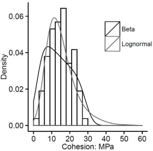
The lognormal and beta distributions were tested forc, φ and E. For all variables it was decided that the beta distribution did not provide a good enough fit to the majority of the data. For example, Figure 3 shows a histogram of cohesion values for mudstone extracted from the CMDB; plotted on the same figure are the theoretical beta and lognormal PDFs. For the majority of the data the lognormal distribution provides a much better fit to the laboratory data. The sensitivity analysis showed that forc, φ and E, the lower values were much more influential; therefore it was deemed that distributions that best fit the lower range of these parameter values were more appropriate. 5.2.2 Probability distribution for GSI
GSI has been defined on a normal distribution, which is justified by considering that it is determined from visual observation and is consequently affected by the subjective judgement of the geologist [12,48]. Hoek [48] therefore suggests that a range of values will be more appropriate than a single ‘exact’ value, with a standard deviation of 2.5, but possibly more in complex geological environments where 2.5 may be too optimistic.
GSI values for the coal measure rocks located at the Thoresby colliery have been suggested [45,49], with values ranging from 49 to 85 for mudstone identified. By selecting the middle of this range, 67, as the mean of a normal distribution with standard deviation of 5 the distribution shown in Figure 5 is produced, covering the range of suggested values. This is quite a conservative approach, but reflects the uncertainty in the GSI parameter that arises in its subjective evaluation in such a complex situation as a deep coal mine.
Parameter Distribution Fitting parameters Plot
E Gamma Shape = 6.212 Rate = 0.385 GPa Figure 2
c Lognormal Mean = 2.594 MPa SD = 0.492 MPa Figure 3
φ Lognormal Mean = 3.374° SD = 0.207° Figure 4
GSI Normal Mean = 67 SD = 5 Figure 5
Table 2: Identified distribution and fitting parameters for those parameters able to be fit with a continuous distribution.
5.2.3 Probability distributions for the stress components
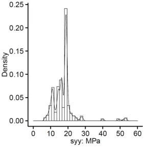
Suitable theoretical, continuous distributions for the stresses have not been found. Figure 3 shows the PDF of syy taken from the Thoresby Colliery FLAC 3D model; similar PDFs were observed for sxx and szz. It is impossible to fit a theoretical model to this distribution; therefore another approach must be taken so that LHS with the inverse CDF method may be applied to the variable, ensuring consistency.
5.3 Sampling, correlation control and analysis monitoring
Table 3 shows how this would be achieved if the distribution was split into strata of 10 MPa. For each strata the probability is calculated, then the cumulative probability. To generate sample values, the randomly generated number, from the uniform distribution [0, 1], is compared to the cumulative probabilities. For example, if the drawn random number is 0.5, the value will be taken from the 10 – 20 strata; if 0.99 it would be taken from the 50 – 60 strata.
syy: MPa Probability Cumulative probability
0 - 10 0.0675 0.0675
10 - 20 0.8313 0.8988
20 - 30 0.0767 0.9755
30 - 40 0.0061 0.9816
40 - 50 0.0061 0.9877
50 - 60 0.0123 1.0000
60 - 70 0.0000 1.0000
Table 3: Discretisation of syy into 10 MPa strata. The cumulative probabilities are used to generate the samples.
2000 samples (meaning a potential of 2000 model runs) are created for each analysis. The variables
E, c, φ and GSI are sampled with LHS, in conjunction with the Inverse CDF method, whereas the
stresses, syy, sxx and szz are all discretised into 0.5 MPa strata and then sampled using LHS with the discretisation method.
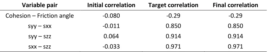
[image:11.595.68.508.603.689.2]In LHScor, the correlation control algorithm is applied to the sample, with the target correlations shown in Table 4. These correlations are entered into the C++ sampling program, from which the target correlation matrix is formed, with correlations of 0.0 for all other parameter pairs.
Table 4 shows the initial and final correlation coefficients between the variable pairs with prescribed correlation, before and after the algorithm was applied. Between all other variable pairs the algorithm acted to remove undesired correlation. Initial correlations between these pairs ranged from -0.079 to 0.064, which could have adversely affected the analysis. Once the algorithm was applied, correlations were reduced to between -0.0002 and 0.0009, with the majority being in the order of between 10-5and10-7.
Variable pair Initial correlation Target correlation Final correlation
Cohesion – Friction angle -0.080 -0.29 -0.29
syy – sxx -0.011 0.850 0.850
syy – szz 0.064 0.914 0.914
sxx – szz -0.033 0.971 0.971
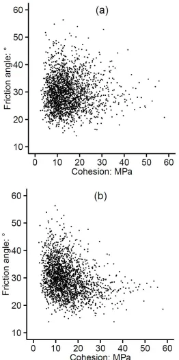
Figure 7a and b show 2000 samples of cohesion – friction angle before (ρ= 0.004) and after (ρ = -0.29) the application of the correlation control algorithm. The samples do appear to be similar but there is a noticeably more negative trend in the correlated sample which, as well as actual measurements of correlation coefficient, shows that the correlation control algorithm was successful.
Each analysis, LHSuncor and LHScor, was set up so that a total of 2000 models could be run. However, it was possible to monitor the results and other measures of quality throughout the runs, so that if decided, analyses could be stopped when the desired accuracy of results was reached. These measures were monitored by using accumulators ܵଵ and ܵଶ [37].ܵଵis the accumulation of each model’s output of roof displacementsݕ, such that the present estimate of the mean value of displacements is given byܵଵ⁄ܰ, where Nis the current number of completed model runs. Theܵଶ accumulator sums the value of each ݕଶ and is used to calculate the relative error, ܴ= ඥܵଶ⁄ − 1ܵଵଶ ⁄ܰ, whereRgives a measure of the statistical precision of the estimated mean value. 5.4 Measured displacements
Figure 8 shows the measured roof displacements obtained from UK Coal’s Thoresby Colliery in DS4 longwall panel’s supply gate. The measurements were made by dual height tell-tales (extensometers), installed at 20 m intervals along the roadway roof at the same time as the installation of the roof bolt support. The two anchor heights of the dual height tell-tales was such that one measured roof movement within the 2.4m roof bolted height and the other roof movement up to 5.0m into the roof; a detailed description of the installation and operation of the tell-tales can be found in [50]. Therefore the plot in Figure 6 shows the total movement, obtained by summing the two values measured by the separate anchors. Note that at some locations along the roadway the measured movement is equal to zero. All values were measured once the roadway was completely excavated.
The results of the two Monte Carlo analyses, LHSuncor and LHScor, will be compared to these central roof displacements. The observed displacements will give a good idea of how well the analyses perform in matching the magnitudes and distribution of the displacements. In the numerical model, central roof displacements were recorded for two separate stages; the first from the beginning of excavation until the installation of roof support and the second from the installation of support until the numerical model reached equilibrium.
The reason for taking this approach is explained by considering the longitudinal displacement profile (LDP) of the roadway. The LDP is the graphical representation of displacements that occur along the axis of an unsupported excavation [51]. The LDP shows that a point within the rock mass, initially well ahead of the advancing roadway face, will have already experienced up to a third of its total displacement once coincident with the face [52]; this quantity is known as the pre-deformation [53]. Numerous equations exist that are used to estimate the LDP of radial displacements for circular tunnels [51,53,54], although they have also been used to estimate the LDP of an almost square tunnel [55].
which is greater than the pre-deformation d0, showing that when the tell-tales are installed it is possible that at least 31% of total displacement, dmax, will already have occurred [51]. The displacement measured by the tell-tales is therefore dmax – dins. Therefore, to ensure that the numerical model provides suitable comparison the displacements were split into two stages. In Section 6, all presented analysis displacements are those measured after the installation of support in the numerical model, the second stage.
6. Results
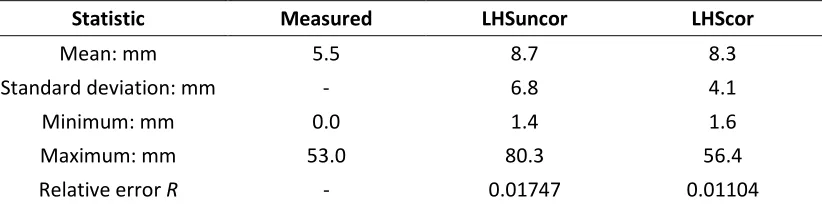
The measurements of central roof displacement, recorded for each model run in the analyses LHSuncor and LHScor, are presented in the form of cumulative distribution functions (CDF) in Figure 10a and b; both are compared to the measured values from the Thoresby roadway (Figure 8). The result statistics are summarised in Table 5. By looking at these plots and the statistics, it is possible to quickly judge the relative performance of each analysis. Overall, analysis LHScor has better matched the measured behaviour, especially in terms of the magnitude of displacements. In LHScor, the maximum values of displacement are 56 mm, comparing more favourably to the observed maximum of 53 mm than the LHSuncor results where they are 80 mm.
Both analyses, when compared to the measured values, overestimate the mean slightly, LHSuncor more so. This is not surprising when looking at the CDFs. The near majority of measured displacements (approx. 50%) are actually zero, whereas in both LHScor and LHSuncor, 50% of the calculated displacements are up to 13mm. Overall, it can be said that the LHSuncor results are slightly more conservative than LHScor considering the maximum displacements and mean value, which, based on the literature, is to be expected.
Statistic Measured LHSuncor LHScor
Mean: mm 5.5 8.7 8.3
Standard deviation: mm - 6.8 4.1
Minimum: mm 0.0 1.4 1.6
Maximum: mm 53.0 80.3 56.4
[image:13.595.72.483.451.554.2]Relative errorR - 0.01747 0.01104
Table 5: Selected statistics of each Monte Carlo analysis after 2000 model runs, compared to the measured results.
At lower values of central roof displacements, the CDFs from the two analyses are very similar, overlapping for displacements less than 15 mm. This suggests that correlation between variables was only influential in affecting the magnitude of higher displacements. Figure 11 goes some way to confirming this, by presenting ranked, from highest to lowest, central roof displacements against a log10scale. The plot shows that it is only within the top 100 greatest displacements where there is a noticeable difference between the correlated and uncorrelated analyses, and the top 50 where this difference is significant.
To have confidence in the results it is important to carry out a post analysis of certain statistics generated during the runs. The evolution of the mean value of each set of roof displacements was recorded, as well as the relative error, using the methods described in Section 5.3. The statistical law of large numbers states that as the size of the sample increases, the mean should tend to a constant value. Therefore it is expected that as the number of model runs increases the mean of the central roof displacements will tend to a constant value.
Figure 12 shows the trend of the mean of the central roof displacements as the number of model runs progresses towards 2000 for LHSuncor and LHScor. There is a clear tendency towards a constant value in both analyses. This trend suggests that the analyses have been successful; telling us that the parameter values have been well sampled from their distributions and that the number of model runs was more than adequate to obtain good mean values.
The relative errorRgives a measure of the statistical precision of the mean value. Dunn and Shultis [37] suggest that a good result should haveܴ≤ 0.05. Table 5 confirms that both analyses have a value ofR well below this threshold, suggesting that confidence can be had in the accuracy of the estimated mean value from each analysis. The slightly higher value for LHSuncor suggests that there is more variance in these results which is confirmed by the values of standard deviation.
7. Discussion
As expected from studying the literature, the analysis not including correlation between parameters was conservative in its results. The maximum displacements in LHSuncor were significantly higher than the maximum values obtained in LHScor and the mean value of displacement was also higher. Due to suggestions and findings of other authors, it was thought that these observations would be due to the included correlation betweenc and φ in the Mohr-Coulomb model. It is suggested here that by including negative correlation between these two parameters, on average, higher values of φ
will have been paired with lower values of c in LHScor, effectively lessening the effects of low cohesion.
To investigate this, the relationship between the parameters and the calculated central roof displacements is considered. This has been achieved by calculating another set of correlations from the results, between each parameter and the calculated central roof displacements. If including negative correlation between c and φ in the analysis does affect the results, noticeably different
correlation coefficients could be expected.
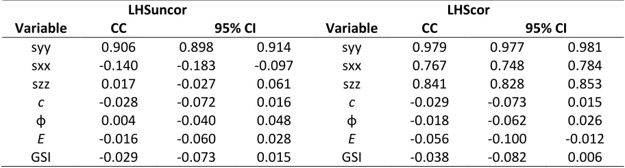
Table 6 presents the correlation coefficient (CC) and 95% confidence interval (CI) of those correlation coefficients, between each parameter and the calculated values of central roof displacements in each analysis. The difference between the correlation coefficients of c-Displacement and φ-Displacement from LHSuncor to LHScor is negligible. The c-Displacement correlation coefficient is
LHSuncor LHScor
Variable CC 95% CI Variable CC 95% CI
syy 0.906 0.898 0.914 syy 0.979 0.977 0.981
sxx -0.140 -0.183 -0.097 sxx 0.767 0.748 0.784
szz 0.017 -0.027 0.061 szz 0.841 0.828 0.853
c -0.028 -0.072 0.016 c -0.029 -0.073 0.015
φ 0.004 -0.040 0.048 φ -0.018 -0.062 0.026
E -0.016 -0.060 0.028 E -0.056 -0.100 -0.012
[image:15.595.64.522.125.248.2]GSI -0.029 -0.073 0.015 GSI -0.038 -0.082 0.006
Table 6: Correlation coefficients and 95% confidence intervals between each model parameter and central roof displacements for LHSuncor and LHScor.
Due to the seemingly negligible effect of includingc – φ negative correlation in the analysis, it seems
likely that there were some other factors influencing the results. Table 6 shows that there is a large difference between the CCs for the stresses between LHSuncor and LHScor. In LHSuncor the correlation between sxx and szz and the total central roof displacements is low, whereas in LHScor they are very strongly positive. This observation suggests that the correlation between the three stresses has affected the results of LHScor.
Figure 13 shows the values of vertical (syy) and horizontal (sxx) stress pairs that resulted in the top 50 largest roof displacements in the LHSuncor and LHScor analyses. There are clearly different values and relationships of the two stresses in each analysis. The spread of sxx is much greater in LHSuncor, whereas in LHScor the magnitude of sxx is centred on 25 MPa. Due to the correlation between stresses in LHScor, higher values of sxx are more likely to be paired with higher values of syy. This is supported by the calculated correlation coefficients for syy-sxx from Figure 13, which are 0.308 for LHSuncor and 0.791 for LHScor. Therefore, it seems that the higher values of sxx in LHScor will lessen the effect of high syy values, which is plausible since the effect is to lessen the magnitude of deviatoric stress within the rock, resulting in fewer occurrences of yield, thereby reducing displacements. It is likely that this effect would not exist if horizontal stresses exceeded the vertical; Lawrence [56] has shown that roadways where horizontal stress exceeds vertical stress can be the worst case in terms of the magnitude of roof instability.
Magnitudes of stress and confining stress also explain the observations made in Figure 11, which showed that there was no difference in the magnitude of displacements between LHSuncor and LHScor below the top 100 displacements. These lower values of displacement occur when the vertical stress is also low, meaning that high confining stress is not particularly necessary to lessen the effects.
[image:15.595.65.521.126.249.2]Despite the best efforts to match the actual situation of excavation and installation of the tell-tales there will still be some discrepancy in the numerical model, which is difficult to avoid, particularly in this simple 2D numerical model. Regarding the statistical distributions, it is noted that the GSI distribution was a conservative estimate due to being based on limited observations and would therefore tend to produce larger displacements. This is not negated by the higher values of GSI (i.e. > mean value) as the initial sensitivity analysis showed that the relationship between GSI and roof displacements is not a linear decrease, but is constant once GSI increases above the mean value (see results in Appendix A).
8. Summary
In this paper, a method for predicting the likely distribution of roof displacements occurring in a deep coal mine roadway has been developed. Two different approaches were taken, each applying the Monte Carlo uncertainty analysis method in differing ways. The first analysis used Latin Hypercube sampling with seven uncorrelated input parameters, the second used the same seven parameters but with correlation included betweenc – φ in the Mohr-Coulomb model and between
stress components.
From the literature, it was expected that the correlation between c – φ could be of major
importance, leading to less conservative results. However, the analysis showed that it actually did not influence the magnitude of displacements. The correlation between the stress components proved to be much more important. By including the strong positive correlation between horizontal and vertical stresses in the correlated analysis, higher values of horizontal stress are more likely to be paired with higher values of vertical stress. This acts to lessen the effects of high vertical stress, by increasing the confining stress.
From these results it is clear that including correlation between the stress components is important to obtain reliable results, particularly from this kind of uncertainty analysis where the aim is to calculate the probability of certain low probability events occurring. If the aim was to simply calculate the mean value then its inclusion, depending on the desired accuracy, may not be as vital. The importance of c – φ negative correlation is much less clear; the correlation coefficients
presented in Table 6 indicate that there was no effect on the analysis. The importance of c – φ
correlation from the literature is inconclusive; more research into this area is required before making any suggestions beyond what have already been made.
Proper definition of the parameter distributions is critical to achieving good results in these types of uncertainty analyses. Lack of access to sufficient quantities of good quality data is a major obstacle which could prevent the use of these methods completely. Availability of a large database of historic laboratory test results meant that confidence in the material property distributions could be had in this work, which subsequently reduced the inherent epistemic uncertainty and gave confidence in the accuracy of results.
it is certainly viable at the planning stage of mine development; with a modern computer good results can be obtained in around one day of model run-time.
Acknowledgements
The authors would like to thank Lorraine Kent of Golders Associates (UK) Ltd for proof reading and her assistance in obtaining the data from Thoresby Colliery, DS4 Longwall panel and to research partner UK Coal Production Ltd for allowing the use of this data. This work has been funded by the European Commission through the collaborative work on the Research Fund for Coal and Steel, Contract RFCR -CT-2013-00001, ‘AMSSTED – Advancing Mining Support Systems to Enhance the Control of Highly Stressed Ground’.
Appendix A
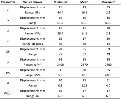
Table A.1 shows the results of the initial sensitivity analysis performed to establish the most important parameters to include in the Monte Carlo analysis. Analyses were carried out on the Young’s modulusE, Poisson’s ratioν, cohesionc, friction angle φ, GSI, density γ, vertical stresssyy, stress ratioK, roadway width and roadway height.
[image:17.595.69.475.436.768.2]For each parameter the minimum and maximum displacement and the displacement at the mean value of the parameter are shown. In the range row for each parameter, the values represent the corresponding parameter value for that displacement; for example the Young’s modulus results show that as the value ofEdecreases the displacements increase.
Table A.1: Results of the initial sensitivity analysis used to choose the relevant parameters for the Monte Carlo analyses.
Parameter Values shown Minimum Mean Maximum
E Displacement: mm 11 13 55
Range: GPa 44.4 16.1 2.8
ν Displacement: mm 15 16 16
Range 0.32 0.18 0.06
c Displacement: mm 15 15 20
Range: MPa 29.7 14.8 2.1
φ Displacement: mm 15 17 30
Range: degrees 50 30 14
GSI Displacement: mm 28 35 69
Range 85 67 49
γ Displacement: mm 14 15 15
Range: kg/m3 2400 2570 2800
syy Displacement: mm 4 30 55
Range: MPa 5.0 32.5 60.0
K Displacement: mm 20 25 51
Range 0.5 2.25 4.0
Height Displacement: mm 14 15 15
Range: m 4.0 3.8 3.6
Appendix B
Table B.1 and B.2 show the statistical parameters for the material properties of the rocks of the UK
[image:18.595.72.522.234.331.2]coal measures, from the CMDB. The selected statistical parameters are the mean μ, standard deviation σ, coefficient of variation COV and the minimum and maximum values.
Table B.1: Statistical parameters for the material properties Young’s modulus and Poisson’s ratio of the UK coal measure rocks, from the CMDB.
Rock type μ Young’s modulus: GPaσ COV Min Max μ σPoisson’s ratioCOV Min Max
Coal 3.07 0.98 0.32 1.1 7.7 0.20 0.01 0.05 0.19 0.21
Mudstone 16.1 6.5 0.40 2.8 44.4 0.18 0.07 0.39 0.06 0.32
Sandstone 18.1 11.3 0.62 4.8 71.7 0.19 0.07 0.37 0.06 0.48
Siltstone 18.0 7.5 0.42 4.8 57.9 0.19 0.05 0.26 0.10 0.35
[image:18.595.67.522.384.480.2]Seatearth 4.7 2.0 0.43 1.1 9.3 0.14 0.13 0.93 0.05 0.32
Table B.2: Statistical parameters for the material properties cohesion and friction angle of the UK coal measure rocks, from the CMDB.
Rock type μ σCohesion: MPaCOV Min Max μ Friction angle: degreesσ COV Min Max
Coal 13.8 4.7 0.34 7.8 18.1 30 7 0.23 22 40
Mudstone 14.8 6.0 0.41 2.1 29.7 30 6 0.20 14 50
Sandstone 13.7 6.7 0.49 1.7 29.2 38 7 0.18 25 61
Siltstone 15.7 7.7 0.49 2.5 41.6 31 7 0.23 16 49
Seatearth 7.1 1.9 0.27 4.4 8.5 25 6 0.24 20 35
Table B.3 and B.4 show the best fit probability distributions for the material properties of the rocks of the UK coal measures, from the CMDB. Distributions have not been provided where the sample size was too small to carry out a reliable fitting process.
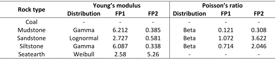
[image:18.595.68.523.647.745.2]For each distribution there are two fitting parameters, FP1 and FP2. For each distribution type these are; beta (FP1 = alpha, FP2 = beta), lognormal (FP1 = mean, FP2 = standard deviation), gamma (FP1 = shape, FP2 = rate) and Weibull (FP1 = shape, FP2 = scale).
Table B.3: Best fit probability distributions for the Young’s modulus and Poisson’s ratio of the UK coal measure rocks, from the CMDB.
Rock type DistributionYoung’s modulusFP1 FP2 DistributionPoisson’s ratioFP1 FP2
Coal - - -
-Mudstone Gamma 6.212 0.385 Beta 0.121 0.308
Sandstone Lognormal 2.727 0.581 Beta 1.072 3.622
Siltstone Gamma 6.087 0.338 Beta 0.714 2.046
-Table B.4: Best fit probability distributions for the cohesion and friction angle of the UK coal measure rocks, from the CMDB.
Rock type Distribution CohesionFP1 FP2 DistributionFriction angleFP1 FP2
Coal - - -
-Mudstone Lognormal 2.594 0.492 Lognormal 2.594 0.492
Sandstone Weibull 2.2 15.5 Lognormal 3.626 0.168
Siltstone Weibull 2.19 17.77 Gamma 20.055 0.649
Seatearth - - -
-References
[1] Hacking I. The emergence of probability. London: Cambridge University Press; 1975.
[2] Baecher GB, Christian JT. Reliability and statistics in geotechnical engineering. Chichester: John Wiley & Sons; 2003.
[3] Christian JT. Geotechnical engineering reliability: how well do we now what we are doing? J Geotech Geoenvironmental Eng 2004;130:985–1003.
[4] Whitman R V. The seventeenth Terzaghi lecture: evaluating calculated risk in geotechnical engineering. J Geotech Eng 1984;110:143–88.
[5] Fenton GA. Probabilistic Methods in Geotechnical Engineering 1997.
[6] Li H-Z, Low BK. Reliability analysis of circular tunnel under hydrostatic stress field. Comput Geotech 2010;37:50–8. doi:10.1016/j.compgeo.2009.07.005.
[7] Kim K, Gao H. Probabilistic approaches to estimating variation in the mechanical properties of rock masses. Int J Rock Mech Min Sci Geomech Abstr 1995;32:111–20.
[8] Griffiths DV, Fenton GA, Tveten DE. Probabilistic geotechnical analysis. Int. Conf. Probabilistics Geotech., vol. 17, 2002. doi:10.1053/j.tvir.2014.08.001.
[9] Helton JC, Davis FJ. Latin hypercube sampling and the propagation of uncertainty in analyses of complex systems. Reliab Eng Syst Saf 2003;81:23–69. doi:10.1016/S0951-8320(03)00058-9.
[10] Lu Z, Reddish DJ, Stace LR. Uncertainty analysis in a numerical modelling context – an example application on a coal mine roadway design. Min Technol 2005;114:232–40.
doi:10.1179/037178405X74068.
[11] Metropolis N, Ulam S. The monte carlo method. J Am Stat Assoc 1949;44:335–41.
[12] Li AJ, Cassidy MJ, Wang Y, Merifield RS, Lyamin AV. Parametric Monte Carlo studies of rock slopes based on the Hoek–Brown failure criterion. Comput Geotech 2012;45:11–8.
[image:19.595.67.524.131.229.2][14] Rohaninejad M, Zarghami M. Combining Monte Carlo and finite difference methods for effective simulation of dam behavior. Adv Eng Softw 2012;45:197–202. doi:10.1016/j.advengsoft.2011.09.023.
[15] Misra A, Roberts L a., Levorson SM. Reliability analysis of drilled shaft behavior using finite difference method and Monte Carlo simulation. Geotech Geol Eng 2006;25:65–77. doi:10.1007/s10706-006-0007-2.
[16] Fenton GA, Griffiths DV. Bearing-capacity prediction of spatially random c − φ soils. Can Geotech J
2003;65:54–65. doi:10.1139/T02-086.
[17] Zevgolis IE, Bourdeau PL. System reliability analysis of the external stability of reinforced soil structures. Georisk 2010;4:148–56. doi:10.1080/17499511003630496.
[18] McKay MD, Beckman RJ, Conover WJ. A comparison of three methods for selecting values of input variables in the analysis of output from a computer code. Technometrics 1979;21:239–45.
[19] Helton JC, Davis FJ. Illustration of sampling-based methods for uncertainty and sensitivity analysis. Risk Anal 2002;22:591–622.
[20] Morin MA, Ficarazzo F. Monte Carlo simulation as a tool to predict blasting fragmentation based on the Kuz–Ram model. Comput Geosci 2006;32:352–9. doi:10.1016/j.cageo.2005.06.022.
[21] Griffiths DV, Fenton GA. Probabilistic slope stability analysis by finite elements. J Geotech Geoenvironmental Eng 2004;130:507–18. doi:10.1061/(ASCE)1090-0241(2004)130:5(507).
[22] Calvo B, Savi F. A real-world application of Monte Carlo procedure for debris flow risk assessment. Comput Geosci 2009;35:967–77. doi:10.1016/j.cageo.2008.04.002.
[23] Griffiths DV, Huang J, Fenton GA. Influence of Spatial Variability on Slope Reliability Using 2-D Random Fields. J Geotech Geoenvironmental Eng 2009;135:1367–78.
[24] Hicks MA, Spencer WA. Influence of heterogeneity on the reliability and failure of a long 3D slope. Comput Geotech 2010;37:948–55. doi:10.1016/j.compgeo.2010.08.001.
[25] Russo G, Kalamaras GS, Origlia L, Grasso P. A probabilistic approach for characterizing the complex geologic environment for design of the new Metro Do Porto 2001;III:463–70.
[26] Valley B, Kaiser PK, Duff D. Consideration of uncertainty in modelling the behaviour of underground excavations. 5th Int. Semin. Deep High Stress Min., 2010, p. 423–35.
[27] Vargas JP, Koppe JC, Pérez S. Monte Carlo simulation as a tool for tunneling planning. Tunn Undergr Sp Technol 2014;40:203–9. doi:10.1016/j.tust.2013.10.011.
[28] Khalokakaie R, Dowd PA, Fowell RJ. Incorporation of slope design into optimal pit design algorithms. Min Technol 2000;109:70–6. doi:10.1179/mnt.2000.109.2.70.
[29] Abdel Sabour SA, Dimitrakopoulos RG, Kumral M. Mine design selection under uncertainty. Min Technol 2008;117:53–64. doi:10.1179/174328608X343065.
[30] Chiwaye HT, Stacey TR. A comparison of limit equilibrium and numerical modelling approaches to risk analysis for open pit mining. J South African Inst Min Metall 2010;110:571–80.
[32] Brown ET. Progress and challenges in some areas of deep mining. Min Technol 2012;121:177–91. doi:10.1179/1743286312Y.0000000012.
[33] Medhurst TP, Brown ET. A study of the mechanical behaviour of coal for pillar design. Int J Rock Mech Min Sci 1998;35:1087–105.
[34] Mark C, Gadde M. Global trends in coal mine horizontal stress measurements. Undergr. Coal Oper. Conf., 2010, p. 21–39.
[35] Coggan J, Gao F, Stead D, Elmo D. Numerical modelling of the effects of weak immediate roof lithology on coal mine roadway stability. Int J Coal Geol 2012;90-91:100–9. doi:10.1016/j.coal.2011.11.003.
[36] Fenton GA, Griffiths DV. Risk assessment in geotechnical engineering. Hoboken: John Wiley & Sons; 2008.
[37] Dunn WL, Shultis JK. Exploring monte carlo methods. Oxford: Academic Press; 2012.
[38] Matsumoto M, Nishimura T. Mersenne Twister : A 623-dimensionally equidistributed uniform
pseudo-random number generator. ACM Trans Model Comput Simul 1998;8:3–30.
[39] Ades AE, Lu G. Correlations between parameters in risk models: estimation and propagation of uncertainty by Markov Chain Monte Carlo. Risk Anal 2003;23:1165–72.
[40] Tang X-S, Li D-Q, Rong G, Phoon K-K, Zhou C-B. Impact of copula selection on geotechnical reliability under incomplete probability information. Comput Geotech 2013;49:264–78.
doi:10.1016/j.compgeo.2012.12.002.
[41] Yucemen MS, Tang WH, Ang A.-S. A probabilistic study of safety and design of earth slopes. 1973.
[42] Cherubini C. Reliability evaluation of shallow foundation bearing capacity on c ′ , φ ′ soils. Can Geotech
J 2000;37:264–9.
[43] Fenton GA, Griffiths DV. Reply to the discussion by R. Popescu on “Bearing capacity prediction of spatially random c - phi soils.” Can Geotech J 2004;369:368–9. doi:10.1139/T03-080.
[44] Vořechovský M, Novák D. Correlation control in small-sample Monte Carlo type simulations I: A
simulated annealing approach. Probabilistic Eng Mech 2009;24:452–62. doi:10.1016/j.probengmech.2009.01.004.
[45] Whittles DN, Lowndes IS, Kingman SW, Yates C, Jobling S. Influence of geotechnical factors on gas flow experienced in a UK longwall coal mine panel. Int J Rock Mech Min Sci 2006;43:369–87.
doi:10.1016/j.ijrmms.2005.07.006.
[46] Itasca. Fast Lagrangian Analysis of Continua (FLAC) ver 6.0. Minneapolis: Itasca Consulting Group; 2008.
[47] Harr ME. Reliability-based design in civil engineering. 1987.
[48] Hoek E. Reliability of the Hoek-Brown estimates of rock mass proerties and their impact on design. Int J Rock Mech Min Sci 1998;35:63–8.
[50] Deep Mines Coal Industry Advisory Committee. Guidance on the use of rockbolts to support roadways in coal mines. Sudbury (UK): HSE Books; 1996.
[51] Carranza-Torres C, Fairhurst C. Application of the convergence-confinement method of tunnel design to rock masses that satisfy the Hoek-Brown failure criterion. Tunn Undergr Sp Technol 2000;15:187– 213. doi:10.1016/S0886-7798(00)00046-8.
[52] Hoek E, Kaiser PK, Bawden W. Support of underground excavations in hard rock. 2000.
[53] Unlu T, Gercek H. Effect of Poisson’s ratio on the normalized radial displacements occurring around the face of a circular tunnel. Tunn Undergr Sp Technol 2003;18:547–53.
doi:10.1016/S0886-7798(03)00086-5.
[54] Chern JC, Shiao FY, Yu CW. An empirical safety criterion for tunnel construction. Reg. Symp. Sediment. Rock Eng., 1998, p. 222–7.
[55] Hoek E. Cavern reinforcement and lining design. 2011.
Figure captions
Figure 1: Diagrams of the Thoresby colliery FLAC 2D numerical model, showing; (a) dimensions and boundary conditions, (b) geological strata surrounding the roadway and (c) the mesh around the roadway, with location of roadway support.
Figure 2: Beta and gamma probability density functions fit to a histogram of the Young’s modulus data from the CMDB. The gamma distribution was chosen for this property.
Figure 3: Beta and lognormal probability density functions fit to a histogram of the cohesion data from the CMDB. The lognormal distribution was chosen for this property.
Figure 4: Beta and lognormal probability density functions fit to a histogram of the friction angle data from the CMDB. The lognormal distribution was chosen for this property.
Figure 5: Normal distribution with mean = 67 and standard deviation = 5 chosen for the GSI variable. Figure 6: Histogram and PDF of vertical stresses, representing how the continuous distribution may be discretised such that the LHS method can still be applied. The plot shows that the majority of stress values are in the range 10 – 20 MPa, with smaller peaks around 40 and 50 MPa, which represent in-situ stresses above the ribs of the previously mined areas in the Parkgate seam. Figure 7: (a) Uncorrelated sample of cohesion - friction angle used in LHSuncor, whereρcφ= 0.005.
(b) Correlated sample of cohesion – friction angle used in LHScor, whereρcφ= -0.29.
Figure 8: Measured roof displacements in the Thoresby Colliery Deep Soft seam supply gate serving longwall panel DS4. Measure mark 0 m represents the entrance of the roadway; therefore
excavation progressed in the direction 0 m to 2500 m.
Figure 9: Possible LDP for the Thoresby colliery roadway. The equation for d0is that of Carranza-Torres and Fairhurst [51].
Figure 10: CDF of central roof displacements for (a) LHSuncor and (b) LHScor, compared to the measured values from the Thoresby Colliery.
Figure 11: Ranked total central roof displacements for both analyses on log10scale.
Figure 1: Diagrams of the Thoresby colliery FLAC 2D numerical model, showing; (a) dimensions and boundary conditions, (b) geological strata surrounding the roadway and (c) the mesh around the roadway, with location of roadway support.
[image:24.595.132.463.376.702.2]Figure 3: Beta and lognormal probability density functions fit to a histogram of the cohesion data from the CMDB. The lognormal distribution was chosen for this property.
[image:25.595.169.431.449.703.2]Figure 5: Normal distribution with mean = 67 and standard deviation = 5 chosen for the GSI variable.
[image:26.595.155.441.394.683.2]Figure 7: (a) Uncorrelated sample of cohesion - friction angle used in LHSuncor, whereρcφ= 0.005.
[image:27.595.167.429.75.601.2]Figure 8: Measured roof displacements in the Thoresby Colliery Deep Soft seam supply gate serving longwall panel DS4. Measure mark 0 m represents the entrance of the roadway; therefore
excavation progressed in the direction 0 m to 2500 m.
[image:28.595.147.444.429.702.2]Figure 11: Ranked total central roof displacements for both analyses on log10scale.
[image:30.595.154.441.399.695.2]