Data collection with in-network fault detection
based on spatial correlation
Lei Fang, Simon Dobson
School of Computer Science
University of St Andrews, UK
Email: [email protected], [email protected]
March 3, 2015
Abstract
Environmental sensing exposes sensor nodes to environmental stresses that can lead to various kinds of sampling failure. Recognising such faults in the network can improve data reliability therefore making sensor net-works suitable candidate for critical monitoring applications. We develop a technique that builds a spatial model of a sensor network and its obser-vations, and show how this can be updated in-network to provide outlier detection even for non-stationary time series. The solution does not re-quire local storage of learning data or any centralised control. The method is evaluated by both real world implementation and simulation, and the results are promising.
Key words: Fault detection, Sensor networks, Online learning, Energy effi-ciency
1
Introduction
Wireless sensor networks (WSNs) are prime candidates for the application of both autonomic and cloud computing techniques. Considered in the large, they observe, collect, and deliver events and/or data from a distributed system to a data store for further analysis. On a small scale, they must function in a hostile environment with limited power budgets, communications and computational capabilities. Since the data observed by WSNs may later be used for scientific or policy purposes, it is vital that the results can be trusted, despite the lack of human-in-the-loop oversight and independent ground truth.
deliberate attack. While the observations of a single node are questionable, the existence of observations from other, nearby nodes observing the same phe-nomena may be used to provide corroborating evidence, allowing the network as a whole to be more accurate than its individual components. The situation is however complicated by two factors. First, the phenomena being observed are by definition dynamic, and may present discontinuous rapid changes be-tween more stable regimes (such as when temperature changes rapidly before a storm). Failing at recognising this change will lead to high false alarm rates, as good data will be classified as faults for its mismatch with the stale model. Second, as resource constrained computing devices, sensors cannot host compu-tational expensive models nor even large scale storage of learning data. Both effects complicate the statistical techniques required, and in particular make in-network decision-making and machine learning more difficult.
Mathematically, the network must process a data stream presenting non-stationary statistical characteristics. The various nodes in the WSN have differ-ent views on the phenomena being observed: some will be independdiffer-ent, others will be correlated, depending both on physical placement and environmental influences. The problem is then to subject this compound system to statisti-cal analysis and develop a model that can autonomously manage and improve the quality of the information being deduced from the raw data streams, which can then either be returned for analysis in the cloud or used for local decision-making.
Sensor data usually exhibits strong spatial correlation: sensor readings mea-sured at close distance are more similar. For example, at a specific time point
s, we should not expect two temperature readings,ti,sandtj,s, measured at
co-located positions,i, j, to deviate significantly. In general, the spatial correlation assumption holds true for most sensor applications, as long as the underlying physical process over the space is continuous.
In this paper, we introduce a novel on-line in-network sensor fault detection algorithm that accounts for spatial correlation. The algorithm autonomously se-lects nodes to be used to verify observed readings, and uses dynamic learning to construct and maintain spatial models of the expected observational correlation. This solution has the following important features.
1. The proposed algorithm performs formal, well-founded fault detection but remain lightweight enough to be carried out locally on resource-constrained sensors. (We have implmented it on TMote Sky nodes.)
3. The learning algorithm is robust to noisy sensor data, working even when faults are present in the training data.
4. The model adapts to the changes in the underlying physical process, so that false positives originating from stale models are minimised.
The structure of the paper is as follows. In section 2 we first present the spatial assumption model used for the algorithm and introduce the fault detec-tion technique in detail in the next secdetec-tion. The combinadetec-tion of the technique with existing data collection protocol as well as implementation details are il-lustrated in section 4. The performance evaluation of the proposed algorithm is presented in section 5. We briefly compare our approach to other related work in section 6 before concluding in section 7 with some future directions.
2
Model Assumptions
Spatial Correlation Model
We use{Yi,t} to denote a time series of observations fort≥0 of some physical variable Y at location i. Given two series {Yi,t} and {Yj,t} of the same
phe-nomenon observed from two locationsiandj, we assume that both are unbiased observations of some true signal plus Gaussian white noise:
Yi,t=µ(xi, t) +t, t iid
∼ N 0, σ21
(1a)
Yj,t=µ(xj, t) +εt, εt iid
∼ N 0, σ22
, (1b)
whereµ(x, t) represents the ground truth of the underlying physical process at the location ofxand time instancet.
For co-located sensorsi, j, we can further assumeµ(xi, t)≈µ(xj, t), as their
distancedij is close. The approximate equality is valid as long as the physical process is diffusive and continuous. Without loss of generality, we assume the true signal difference is a small constantδij =µ(xi, t)−µ(xj, t).
The spatial model simply states that for any two co-located sensor series
{Yi,t}and{Yj,t}, the synchronised difference{et=Yi,t−Yj,t, t≥0} is a Gaus-sian random variable. That is to say,
etiid∼ N(δij, σ2e). (2)
The model can be easily verified given (1). Note that the varianceσ2
e can be treated as a known constant in most WSN
context, sinceσ2
e = Var[−ε] =σ21+σ22, whereσiis the measurement uncertainty
System Assumptions
The following assumptions are made in addition to the spatial correlation as-sumptions from above:
• We consider monitoring applications of WSNs, which require designated sensor nodes continuously to send back real-time sampled sensor data to one or more sinks. We assume that an appropriate routing protocol exists that can direct message flows from each local node to a sink.
• The network topology is assumed to be set in advance and known by local sensor nodes. This assumption is usually true for static WSN deployments, although not for, for example, air-deployed networks.
• Local synchronisation is maintained by local sensor clusters. Time syn-chronisation can be easily achieved by adding an integer type value into radio messages [1].
It is also advantageous (although not required) that the specification of the hardware – the mote and sensor chips – used in the deployment is known be-forehand. However, the relevant parameters can be estimated from sensor data if no such description is available.
3
Statistical model
3.1
Two Inference Problems
The proposed solution revolves with two sub-problems. The first is verifier selection: each source node needs to find its qualified verifier nodes in the sense that valid spatial correlation is held between their data traces. Second, after the appropriate verifiers are selected, how the sampled sensor data at source node can be validated. We are going to show these two problems can be solved as probabilistic inferences by formal statistical tests.
Verifier Node Selection
The problem can be defined as follows: Given a sensor network that continuously monitors a continuous physical variable, for each nodeiwith physical neighbours
Nbr(i), design a distributed algorithm to find a subsetV rf(i)⊆Nbr(i) such that the spatial correlation is valid.
Based on the spatial assumption model, δij, the true signal difference be-tween two co-located sensors, should be a small quantity for spatial correlated nodes, i.e. they are essentially measuring the same phenomenon with marginal difference. Therefore, to filter out irrelevant nodes, one only needs to make inference on the size of δij. Formally we set P(|δij| < ∆µ|e1:n) ≥ 0.95 for
some predefined small constant ∆µ in order to get the standard 95% confidence
interval. In Bayesian terms, the distribution, δij|e1:n, is called the posterior
distribution.
Fault Detection
After the verifier node selection step, each source nodeinow has the knowledge of its data verifier setV rf(i). The problem of fault detection can be formed as follows: For a source nodeiand collected sensor readingYi,t, given its verifiers V rf(i) and their sensor readings Yj,t, j ∈ V rf(i), design a distributed data validation algorithm to test whetherYi,t is sensor data fault or not.
To validate new sensor readings, instead of making inference on δij, the hidden physical signal, we are going to make inference on the new observation
en+1 =Yi,n+1−Yj,n+1 directly. The distribution of en+1 given historical data
set e1:n, i.e. en+1|e1:n is calledpredictive distribution. Based on it, the fault
detection problem can be solved by calculating the probability of observing the new data: if the chance is small then it should be classified as a fault and vice versa.
In summary the solution boils down to two steps:
1. learn the relevant probability distributions; and then
2. solve the problems by forming statistical tests.
The detailed tests which depends on the distributions, are presented later in section 3.3 after the model learning algorithms are introduced.
3.2
Learning model
Efficient Online Learning
In this section, we are going to show the two distributions can be learnt in a on-line sequential way with minimum computational overhead and constant storage requirement, which is desirable for resource constrained devices like sensors.
According to Bayesian statistics, one can show that, by using uninformative prior [2, 3, 4]:
1. The posterior is
δij|e1:N ∼ N
ˆ
µ,σ
2
e N
; (3)
2. The prediction is
eN+1|e1:N ∼ N
ˆ
µ,(N+ 1)σ
2
e N
; (4)
where ˆµ, N1 PN
i=1ei.
Case 2: σe is unknown
1. The posterior distribution is Student T distributed with mean ˆµ, variance sN2, andN−1 degree of freedom
δij|e1:N ∼ T(ˆµ, s2
N, N−1); (5)
2. The prediction is
eN+1|e1:N ∼ T(ˆµ,(N+ 1) s2
N, N−1); (6)
wheres2
, N1−1
PN
i=1(ei−µˆ)2
To put this another way, we predict the expected signal difference and noise-driven error using a distribution learned in the previousN steps. Note that Case 2 distributions share the same mean but use an estimators2instead of the known variance, comparing with Case 1. For both cases, the predictive distributions are identical to their posterior counterparts except the inflated variances (by a factor ofN+ 1). Therefore, one only needs to learn the shared parameters once to obtain the two distributions.
It can be shown that the distributions for both cases can be learnt efficiently with linear growth time complexity and constant memory storage. Theorem 1 shows this claim.
Theorem 1 (Efficient Model Learning). The posterior distribution δij|e1:N ∼
T(ˆµ,sN2, N−1) can be learnt in an on-line fashion with space complexityΘ(1),
and time complexityΘ(N)via the following recursive procedure:
¯
µn= ¯µn−1+
1
n(en−µn¯ −1), (7a)
Sn=Sn−1+ (en−µn¯ −1)(en−µn¯ ), , (7b)
s2(n) = Sn
n−1 (7c)
and
ˆ
µ= ¯µN and s
2
N =
SN
Proof. By defining ¯µ1 = e1 and S1 = 0, for 1 < k ≤ N, ¯µk and Sk can
be calculated at constant cost as a sum of ¯µk−1, Sk−1 and an adjusting term
involvingek. The time complexity is Θ(N) fork=N. Throughout the process,
three parameters ¯µk, Sk and ek are maintained, so the space complexity is of Θ(1). The proof of the given recursive procedures is omitted due to space limit.
The learning formula for Sn is due to Knuth [5]. There are other one-pass algorithms for computing sample variance, notably
Sn=
n
X
i=1
e2i −
1
n
n X
i=1
ei
2
However, this equation needs to maintain two additional parameters in memory and then perform the subtraction of two substantial sums, which risks larger relative error.
Robust Learning by Markovs’ Inequality
Just like normal sensor data, the learning data is subject to faults as well. We believe the assumption of error free learning data is not realistic; therefore, an additional step of error data filtering is added to make the algorithm robust. The filtering test applies Markov’s inequality.
Theorem 2 (Markov’s Inequality). Let ξ be a non-negative random variable
and its meanE[ξ]exists, For anyt >0
P(ξ > t)≤E
[ξ]
t (9)
Proof. Sinceξ >0,
E[ξ] =
Z +∞
−∞
ξp(ξ)dξ=
Z +∞
0
ξp(ξ)dξ=
Z t
0
ξp(ξ)dξ
+
Z +∞
t
ξp(ξ)dξ≥
Z +∞
t
ξp(ξ)dξ≥t
Z +∞
t
p(ξ)dξ
=tP(ξ > t).
Let ξ = (ei−µ¯n)2, then its mean E[ξ] can be estimated by ¯µξ = Snn =
1
n
Pn
i=1(ei−µn¯ )
2. When a new learning data entryekis arrived, the probability
of observing some value as extreme as it isP(ξ > ξk) whose value is smaller than
¯
µξ/ξk, whereξk = (ek−µk¯ −1)2. By selecting a test probability threshold like
pthred= 1%, we can filter out the noisy learning data. Note that the filtering test
3.3
Statistical Tests
Verifier Node Selection Test
As discussed in Section 2, to find spatial correlated nodes, one only needs to make inference on δµ by calculating the probability P(|δµ| < ∆µ|e1:N) and
comparing it with some predefined confidence level. The exact probability can be calculated by integration. However, to ease the computation, we instead derive the following test rule.
Theorem 3(Verifier Node Test). If
Case 1: δij|e1:N ∼ N
ˆ
µ,σ2e
N
,
ˆ
µ+tα,∞
r
σ2
e
N <∆µ and µˆ−tα,∞
r
σ2
e
N >−∆µ, (10)
Case 2: δij|e1:N ∼ T(ˆµ,s
2
N, N−1),
ˆ
µ+tα,N−1
r
s2
N <∆µ and µˆ−tα,N−1
r
s2
N >−∆µ, (11)
then
P(|δij|<∆µ|e1:N)≥1−2α, (12)
where∆µ is a positive constant, andtα,N−1 is the critical percentile value from
the corresponding Student T distribution. tα,∞ is the Gaussian counterpart.
Proof. The transformed random variable
δij−µˆ
p
s2/N
e1:N ∼ T(0,1, N−1).
SoP(−tα,N−1< √δij−µˆ
s2/N
< tα,N−1|D) = 1−2α, leading to
P µˆ−t
r
s2
N < δij <µˆ+t
r s2 N D !
= 1−2α.
If (11) holds, then
P(|δij|<∆µ|D) =P µˆ−t
r
s2
N < δij <µˆ+t
r s2 N D !
+P −∆µ< δij≤µˆ−t
r s2 N D !
+P µˆ+t
r
s2
N ≤δij<∆µ
D !
By the converging property for Student T distribution, the proof for case 1 follows by settingN=∞.
According to Theorem 3, there are three user controlled parameters: the learning data size N, critical percentile value tα,N−1 and predefined spatial
difference threshold ∆µ. Some general rule of thumbs can be applied to select
them. For example, confidence intervals of 95% and 90% (α= 0.025 or 0.5) are commonly used in statistical tests. Learning data size should be relative large number, such asN≥500, which implies a more stable learnt model but also the Student T distribution converges to a Gaussian distribution: the corresponding Gaussian critical values can be used instead. The spatial difference threshold ∆µ is used to specify how close co-located sensor readings are. Some expert
field knowledge or even common sense can guide the selection of the value. For example, for a normal sensor application with average node distance of 10 meters, we should not expect two co-located temperature readings differ by 1℃.
Data Fault Test
The following theorem presents the statistical test to find out whether a new observation is faulty or not. A positive result from the test implies the proba-bility of observing a value as extreme as the current one is small. The theorem actually rephrases a regular Student t-test, whose proof is omitted.
Theorem 4(Data Fault Test). Given observationsYi,N+1,Yj,N+1from sensor
i,j,∆N+1=Yi,N+1−Yj,N+1, and nodej ∈V rf(i). If
Case 1: eN+1|e1:N ∼ N
ˆ
µ,(N+ 1)σ2e
N
,
ˆ
µ+tα,∞
r
(N+ 1)σ
2
e
N <∆N+1
_
ˆ
µ−tα,∞
r
(N+ 1)σ
2
e
N >∆N+1, (13)
Case 2: eN+1|e1:N ∼ T(ˆµ,(N+ 1)s
2
N, N−1),
ˆ
µ+tα,N−1
r
(N+ 1)s
2
N <∆N+1
_
ˆ
µ−tα,N−1
r
(N+ 1)s
2
N >∆N+1, (14)
then
Multiple Verifiers Test For multiple verifiers, we can collect verification information from all (or a sub-set) ofvrf(i): if at least one verification result supports the suspect data, we mark the data as non-faulty. This mechanism protects against the risk of the breakdown of pairwise spatial correlations, since the synchronised differenceetis only partially stationary, meaning that, which
et remains stationary locally, it still evolves over the long term resulting in a
learned historic model breaking down over time. It is substantially less likely that a node’s observation will betotallydifferent from those ofallits neighbours. The following test rule is used.
faulty : if
vrf(i)
^
j=1
boolj(Yi,t) ==true (16)
3.4
Spatial model update
After the modeleN+1|{Yi,t}is learned initially from the first batch ofN
obser-vations, it needs to be updated as more data are observed. There are essentially three reasons for updating:
1. The spatial difference et is only partially stationary, and so will evolve over time and invalidate the learned model;
2. Future data provide improved temporal correlations, allowing inference on the whole observed data series rather than only on the learned prefix; and
3. The computational effort involved in updating the model is significantly less than that involved in learning a new model from scratch if the initial model becomes outdated.
We further argue that only the mean estimator ˆµneeds to be updated, while the variances2 can be ignored. Under our spatial assumption, σ
e representing
Time
ei
0 200 400 600 800 1000 1200
0.05
0.10
0.15
0.20
0.25
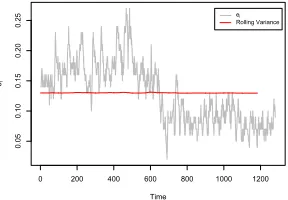
[image:11.612.231.375.133.233.2]ei Rolling Variance
Figure 1: Spatial difference sensor dataei with its mean adjusted rolling
vari-ance.
Obviously only data classified as non-faulty should be admitted into the model as it is updated. We reuse the test in Theorem 4 to check the eligibility of a data entryetto be incorporated into the model. However, a different, or more
conservative, critical valuetα should be used. The motivation is to protect the model update from over data selection. For example, if 90% confidence interval was used, then there would be approximately 10% of good data being excluded from update. To differentiate these two thresholds, we denote the significance level used for update selection asαupdateandαftestfor the other.
Temporally close observations should resemble each other in the same way as spatially close observations. Another way of looking at this is that different elements of{Yi,t}carry different amounts of information. Therefore, for predic-tion, each data entry ine1:N carries a different level of information. It is natural
to give them varying weights based on this correlation.
Note the model update procedure for the mean in Theorem 1, however, gives equal weights. To see this, the formula can be rewritten as
¯
µn= n−1
n (
n−2
n−1µn¯ −2+ 1
n−1en−1) + 1
nen
= 1
nen+
1
nen−1+
1
nen−2+. . .
We use the following recursive formula instead to update the model to take temporal correlation into account. The modified procedures provide estima-tors with time varying weighting such that newer data entries are given higher weights.
˜
µn= ˜µn−1+ψ(en−µn˜ −1) (17)
Note that (17) can be rewritten as ˜µn =ψen+ (1−ψ)˜µn−1. By induction, it
can be shown that
˜
µn=ψen+ (1−ψ)ψen−1+. . .+ (1−ψ)ne0
=
n
X
i=1
(1−ψ)n−iψei+ (1−ψ)ne0=
n
X
i=0
wiei,
where w0 = (1−ψ)n, wi = (1−ψ)n−iψ for 1 ≤ i ≤ n. The time varying
weighting is evident as the weight decays exponentially as time traces back. Note that ˜µn is a convex combination of the observations, i.e. the weights sum to one, which makes ˜µn an unbiased estimator.
Weight
0.00
0.02
0.04
0.06
Weight
0.00
0.05
0.10
0.15
[image:12.612.227.371.284.413.2]Time
Figure 2: Time Varying Weights with ψ = 0.1 (top) and ψ = 0.3 (bottom) respectively.
The smoothing constant, ψ, is a user controlled parameter. As can be seen from Figure 2, large ψ, leading to a lighter tail, will give recent observations heavier weights. In other words, differentψwill make the system responsive to physical process changes at different rates. To help user specify the value, the following heuristic rule is derived.
The sum of partial weights on thek recent observations is
n
X
i=n−k+1
wi=ψ
1−(1−ψ)k
1−(1−ψ)
= 1−(1−ψ)k;
Therefore, the weights over the firstn−k historic data are given by
W(ψ) = (1−ψ)k.
15 seconds. It is safe to assume observations within 10 minutes lag are more temporal correlated; so we should setk= 40. Therefore, selectingψ= 0.3 will make sureW(ψ)≈0.
4
Protocol Design and Implementation
[image:13.612.222.387.244.344.2]In this section, we present how the technique is incorporated into existing WSN data collection protocols.
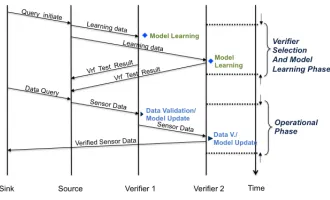
Figure 3: An Overview of the Message Passing Sequence.
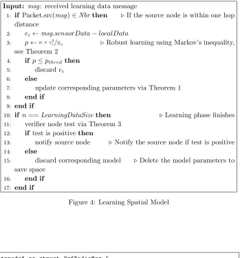
A sequence diagram showing the whole life cycle of the proposed solution is listed in Figure 3. The whole data collection procedure starts with a learning phase, in which the objective is to learn the two distributions, which later will be used for the verifier selection test and fault detection in operational phase. More specifically, the relevant source nodes broadcast its sensor readings to its one-hop distance neighbours as learning data. Each potential verifier then learns the corresponding spatial modelvia (7). After a model with a predefined amount of learning data is learnt, each potential verifier carry out the verifier selection test by Theorem 3. The test result, if positive, is sent back to the corresponding source node. Upon this point, each source node and its corresponding eligible verifier nodes have established their source-verification relationships. Note that we differentiate source node and verifier node here only for the sake of clar-ity; however, each sensor can serve as both roles at the same time. Figure 4 summarises the steps involved in the learning phase.
Input: msg: received learning data message
1: if Packet.src(msg)∈Nbrthen . If the source node is within one hop distance
2: ei←msg.sensorData−localData
3: p←n×e2i/Sn .Robust learning using Markov’s inequality,
see Theorem 2
4: if p≤pthred then
5: discardei
6: else
7: update corresponding parameters via Theorem 1
8: end if
9: end if
10: if n==LearningDataSize then . Learning phase finishes
11: verifier node test via Theorem 3
12: if test is positive then
13: notify source node .Notify the source node if test is positive
14: else
15: discard corresponding model .Delete the model parameters to save space
16: end if
[image:14.612.133.482.146.520.2]17: end if
Figure 4: Learning Spatial Model
t y p e d e f n x _ s t r u c t V r f R a d i o M s g {
n x _ u i n t 1 6 _ t id ; /* N o d e id of s o u r c e m o t e . */
n x _ u i n t 1 6 _ t c o u n t ; /* E p o c h c o u n t */
n x _ u i n t 8 _ t q I n d e x ; /* F r o n t of t h e v r f q u e u e */
n x _ u i n t 8 _ t q S i z e ; /* T h e s i z e of t h e q u e u e */
n x _ u i n t 1 6 _ t v r f Q u e u e [ M A X _ N B R S I Z E ]; /* V e r i f i e r a d d r s Q u e u e */
n x _ u i n t 1 6 _ t v o l t a g e ;
n x _ u i n t 1 6 _ t s e n s o r D a t a ; /* S e n s o r d a t a f r o m s o u r c e */
n x _ u i n t 8 _ t v r f R s t ; /* A B o o l e a n f l a g s t h e v r f r e s u l t so f a r */
} V r f R a d i o M s g _ t ;
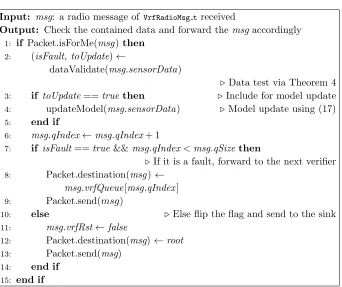
message destination either to the next verifier in the queue, or the sink, if the test result is negative, i.e. not faulty. The data message will finally be delivered to the sink by normal WSN routing protocols such as the Collection Tree Protocol [7]. The verifiers who test the data also need to update its local model according to (17). To give each verifier equal chance to update their local models and, more importantly, to balance the work load, it is advisable for the source node to change the verifier sequence queue from time to time by rotating the queue or even shuffle the sequence. The algorithm for data validation procedure is summarised in Figure 6.
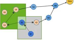
[image:15.612.233.379.379.458.2]Figure 5 shows an example of deployment featuring the proposed data validation technique. There are two source nodes, S1 and S2; each with its verifier node set {S2, V2} and{V3, V4, V5} respectively. Note thatS2 serves as both source node and verifier node forS1 in this case. We use hollow arrows to represent the message passing for local data validation; while the regular arrows are used to mark the message relay to the sink. In this case,S2 sets its verification sequence as [V3, V4, V5]. However, the group validation mechanism finalises its decision before reachingV5; therefore, the verified data is enroute to the sink directly.
Figure 5: A WSN Deployment with Spatial Fault Detection
5
Evaluation
We access the solution in various aspects. First, to show the proposed algorithm is lightweight enough to run in sensors, we implement the solution and deploy it to sensor nodes. Second, numeric simulation is done to access the detection accuracy.
5.1
Implementation
Input: msg: a radio message of VrfRadioMsg treceived
Output: Check the contained data and forward themsgaccordingly 1: if Packet.isForMe(msg)then
2: (isFault, toUpdate)←
dataValidate(msg.sensorData)
. Data test via Theorem 4
3: if toUpdate==true then . Include for model update
4: updateModel(msg.sensorData) .Model update using (17)
5: end if
6: msg.qIndex←msg.qIndex+ 1
7: if isFault==true &&msg.qIndex<msg.qSizethen
. If it is a fault, forward to the next verifier
8: Packet.destination(msg)←
msg.vrfQueue[msg.qIndex]
9: Packet.send(msg)
10: else .Else flip the flag and send to the sink
11: msg.vrfRst←false
12: Packet.destination(msg)←root
13: Packet.send(msg)
[image:16.612.138.480.241.528.2]14: end if 15: end if
Table 1: Program Size Comparison
Without SDV SDV (increase) P. of total
RAM (in Bytes) 492 576 (17%) 5.6%
ROM (in Bytes) 15860 20872 (24%) 42.5%
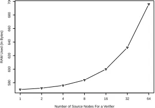
processor running at maximum 8MHz and RAM of 10 KB [9]. The relative small RAM size becomes a major hindrance for the system and application program. The footprint of a typical node which serves as both source and verifier is reported in Table 1. Comparing with a pure data collection implementation, a marginal increase of 17% in RAM with the spatial data validation (SDV) augmented solution is observed. Actually, the program size only depends on the number of spatial models kept locally, Figure 7 shows this relationship. Note that even for the extreme case of 64, i.e. a verifier serving 64 source nodes at the same time, the RAM is 696 bytes, only constituting 6.8% of the total memory (the ROM is 20876 bytes).
580
600
620
640
660
680
700
Number of Source Nodes For a Verifier
RAM Used (In Bytes)
1 2 4 8 16 32 64
Figure 7: Memory Footprint of the Solution Versus the Number of Local Spatial Models
5.2
Numerical simulation
To better understand the detection accuracy of the solution, we use a real-world data set: the Intel Lab Data [6] to run numerical simulation. All the experimental results are obtained from simulations written in R [10]. The user controlled parameters used for the evaluation are listed in Table 2.
[image:17.612.229.380.365.470.2]Table 2: A Summary of Key Parameters
Name Value Used Description
N Learning data size 500
pthred Probability threshold set to
fil-ter out erroneous learning data; see Section 3.2
1%
∆µ Spatial difference threshold for
co-located sensor readings
0.5℃
αvtest Significance level set for verifier
selection test
0.25%
αf test Significance level set for data val-idation test
0.25%
αupdate Significance level set for selected
update test
0.05%
ψ Decaying parameter set for time varying parameter update
0.3
Table 3 summarises the definitions, models and the parameters used for the different faults. The parameters are selected based on existing works [11, 12].
Detection Accuracy The faults detected mainly can be categorised into the following four classes: data points correctly detected as faulty (true positive, TP); data points correctly detected as non-faulty (true negatives, TN); data points incorrectly detected as faulty (false positives, FP); and data points in-correctly detected as non-faulty (false negatives, FN). Two simulation scenarios are considered:
1. Injecting errors only in source nodes;
2. Injecting errors in both a source node and its neighbours.
Two measurements, sensitivity and specificity, are reported. Note that
Sensitivity = TP
TP + FN (18)
Specificity = TN
FP + TN. (19)
Table 4: Simulation Results of Detection Accuracy
SHORT CONST. NOISE DRIFT
CASE 1 Sens. 1.0 1.0 0.774 0.996
Spec. 1.0 1.0 1.0 1.0
CASE 2 Sens. 1.0 1.0 0.682 0.996
Spec. 0.999 0.999 0.999 0.999
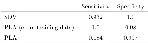
Table 5: Comparing with PLA
Sensitivity Specificity
SDV 0.932 1.0
PLA (clean training data) 1.0 0.98
PLA 0.184 0.997
correctly identified. On the other hand, specificity measures the proportion of negatives, i.e. innocent sensor data, which are correctly identified as such; there-fore, good specificity also means low false positive rate. According to Table 4, we observe the solution performs well for Short, Constant, and Drift fault types. It successfully detects almost all the faults but keeps the false positive rate low. For case two, the performance degrades a bit when faults are introduced to ver-ifiers as well. However, because of the employed Multiple Verver-ifiers Test, the risk of detection errors is shared among the verifiers, leading to a minor degradation. The relative poor performance of fault type Noise is due to the fact that the added noises are zero mean Gaussian samples, which lead to minor faults, i.e. deviating too marginally from the truth to be identified as a fault.
The good specificity means the solution has a very low false positive rates. As pointed in [13, 14], false positives are usually caused by mismatching detection models. As sensor data is always evolving, models learnt by historic data, if not updated, will not commensurate with the changing phenomenon, leading to false positives. The relative low FP rate is attributed to the employed time varying model update procedure, which makes the spatial model adaptive to the changing phenomenon. Figure 8 shows an example of this adaptiveness. The upper figure shows the evolution of a pair of sensor data; while the second figure shows the corresponding spatial differenceet, and the solution successfully catches this evolution by updating its model parameter (the red line)via (17).
[image:20.612.183.424.266.337.2]T
emper
ature
0 200 400 600 800 1000
18
20
22
24
26
Time ei
0 200 400 600 800 1000
−0.5
0.0
0.5
1.0
1.5
2.0
[image:21.612.219.390.124.258.2]Diff Updated Mean
Figure 8: Time Varying Model Update
this effect by injecting errors into learning data set and compare the perfor-mance with the solution proposed in [11]. The method [11], called PLA here, employs a ad hoc heuristic rule to derive the faulty data threshold. As shown in Table 5, after introducing errors into learning data, the performance degrades in sensitivity (decrease 6.8%) while the false positive rate is still great. On the other hand, PLA suffers a more severe sensitivity degradation (over 81.6%) in comparison with its error free learning counterpart.
6
Related work
Ni [15] presents a detailed taxonomy of sensor data faults; however, no detailed detection method is proposed. Sharma [12] also studies data faults, as well as their possible causes. Four different data fault detection methods are com-pared: heuristic methods, estimation methods, time series analysis methods, and learning-based methods. The authors found that these four classes sit at different points on the detection accuracy spectrum. But none of the four are on-line and distributed solutions neither not adaptive. They depend heavily on domain/expert knowledge to set learning parameters beforehand rather than adjusting the learned model adaptively. A good survey on outlier detection techniques is presented by Zhang et alia [16], although most of the solutions work off-line.
suf-fer from memory explosion [17]. An alternative solution [18] presents a on-line solution based on statistical tests and the technique can distinguish between erroneous measurements and events. However, no flexible adaptive procedure is given to update the model and no details on the integration of the solution and existing data collection protocol is presented.
7
Conclusion
We have proposed an online, distributed fault detection technique. The solution is lightweight and integrates well with existing data collection protocols for WSNs. To make the solution adaptive to the changing physical phenomenon, we make use of a time varying model update procedure. Simulation results show that the solution can effectively detect short, constant, and drift faults. We have also implemented the solution on real-world sensors, with a memory footprint less than 6% of the total available memory.
Some parts of the solution still need further investigation. For instance, due to time limits, we only implemented the core part of the solution and no compre-hensive evaluation on the real-world deployment has been carried out. Because ground truth for regular sensor data is missing, most fault detection works are evaluated by injecting artificially-created faults. However, we think it would be better to directly apply the solution blindly to original sensor data and compare the result over different solutions. For example, we may compare the test result of our computationally cheap solution with more complex solutions featuring more sophisticated statistical models, like Gaussian process or Bayesian space-time models, computed at server-side. The sophisticated solutions can serve as reference models in the absence of ground truth.
References
[1] P. Levis and D. Gay,TinyOS programming. Cambridge University Press, 2009.
[2] D. S. Sivia, Data analysis: a Bayesian tutorial. Oxford university press, 1996.
[3] K. P. Murphy,Machine learning: a probabilistic perspective. MIT Press, 2012.
[4] G. Petris, S. Petrone, and P. Campagnoli,Dynamic linear models with R. Springer, 2009.
[5] D. E. Knuth, “The art of computer programming, 3rd edn., vol. 2,”
[6] INTEL, “Intel Berkeley Laboratory sensor data set,” http://db.csail.mit.edu/labdata/labdata.html, 2004.
[7] O. Gnawali, R. Fonseca, K. Jamieson, D. Moss, and P. Levis, “Collection tree protocol,” in Proceedings of the 7th ACM Conference on Embedded
Networked Sensor Systems. ACM, 2009, pp. 1–14. [Online]. Available:
http://dl.acm.org/citation.cfm?id=1644040
[8] P. Levis, S. Madden, J. Polastre, R. Szewczyk, K. Whitehouse, A. Woo, D. Gay, J. Hill, M. Welsh, E. Brewer, and D. Culler, “TinyOS: An Operating System for Sensor Networks,” in Ambient
Intelligence, W. Weber, J. Rabaey, and E. Aarts, Eds. Berlin/Heidelberg:
Springer Berlin Heidelberg, 2005, ch. 7, pp. 115–148. [Online]. Available: http://dx.doi.org/10.1007/3-540-27139-2 7
[9] Moteiv, Tmote Sky Datasheet
http://www.sentilla.com/pdf/eol/tmote-sky-datasheet.pdf, 2006.
[10] R Core Team,R: A Language and Environment for Statistical Computing, R Foundation for Statistical Computing, Vienna, Austria, 2012, ISBN 3-900051-07-0. [Online]. Available: http://www.R-project.org
[11] A. R. M. Kamal, C. Bleakley, and S. Dobson, “Packet-Level Attestation (pla): A framework for in-network sensor data reliability,” ACM Trans.
Sen. Netw., vol. 9, no. 2, pp. 19:1–19:28, Apr. 2013. [Online]. Available:
http://doi.acm.org/http://dx.doi.org/10.1145/2422966.2422976
[12] A. Sharma, L. Golubchik, and R. Govindan, “Sensor faults: Detection methods and prevalence in real-world datasets,” ACM Transactions on
Sensor Networks, vol. 6, no. 3, pp. 23–33, 2010.
[13] J. Gupchup, A. Sharma, A. Terzis, A. Burns, and A. Szalay, “The perils of detecting measurement faults in environmental monitoring networks,”
in Proceedings of the International Workshop on Wireless Sensor Network
Deployments (WiDeploy), 2008.
[14] L. Fang, S. Dobson, and D. Hudges, “An error-free data collection method exploiting hierarchical physical models of wireless sensor networks,” in
Proceedings of the 10th ACM Symposium on Performance Evaluation of
Wireless Ad Hoc, Sensor, & Ubiquitous Networks, ser. PE-WASUN
’13. New York, NY, USA: ACM, 2013, pp. 81–88. [Online]. Available: http://doi.acm.org/10.1145/2507248.2507255
“Sensor network data fault types,” ACM Transactions on Sensor
Networks, vol. 5, no. 3, pp. 25:1–25:29, 2009. [Online]. Available:
http://doi.acm.org/10.1145/1525856.1525863
[16] Y. Zhang, N. Meratnia, and P. Havinga, “Outlier detection techniques for wireless sensor networks: A survey,” Communications Surveys Tutorials, IEEE, vol. 12, no. 2, pp. 159–170, 2010.
[17] E. Elnahrawy and B. Nath, “Context-aware sensors,” inWireless Sensor
Networks. Springer, 2004, pp. 77–93.