Prototype for Multidisciplinary Research
in the context of the Internet of Things
Miguel López-Benítez
∗, Timothy D. Drysdale
†, Simon Hadfield
‡and Mohamed Ismaeel Maricar
§ ∗Department of Electrical Engineering and Electronics, University of Liverpool, United KingdomEmail: [email protected]
†Department of Engineering and Innovation, The Open University, United Kingdom
Email: [email protected]
‡Centre for Vision, Speech and Signal Processing, University of Surrey, United Kingdom
Email: [email protected]
§George Green Institute for Electromagnetics Research, University of Nottingham, United Kingdom
Email: [email protected]
Abstract—The Internet of Things (IoT) poses important challenges requiring multidisciplinary solutions that take into account the potential mutual effects and interactions among the different dimensions of future IoT systems. A suitable platform is required for an accurate and realistic evaluation of such solutions. This paper presents a prototype developed in the context of the EPSRC/eFutures-funded project “Internet of Surprise: Self-Organising Data”. The prototype has been designed to effectively enable the joint evaluation and optimisation of multidisciplinary aspects of IoT systems, including aspects related with hard-ware design, communications and data processing. This paper provides a comprehensive description, discussing design and implementation details that may be helpful to other researchers and engineers in the development of similar tools. Examples illustrating the potentials and capabilities are presented as well. The developed prototype is a versatile tool that can be used for proof-of-concept, validation and cross-layer optimisation of multidisciplinary solutions for future IoT deployments.
I. INTRODUCTION
Communication networks no longer connect just people, but are evolving into billions of interconnected smart devices (sensors, controllers, machines, autonomous vehicles, drones, etc.) [1], with embedded electronics and a number of com-mon basic functionalities (communications and networking protocols, operating systems and software). These objects are interconnected anytime and anywhere with the aim of enabling the automatic collection and exchange of data (possibly with little or no human intervention). This concept, known as the Internet of Things (IoT) [2–4], virtually allows any object to be sensed and controlled remotely across existing network in-frastructure, creating unlimited opportunities for the integration of the physical world into automated computer-based systems equipped with intelligence and smart features.
IoT is seen as the next stage of the information revolution and, with an estimated 50 billion devices connected by 2020 [5], it is becoming a reality. IoT has the potential to revo-lutionise our lives through many applications in future smart cities, composed of smart domains such assmart homes,smart e-healthcare,smart transportation,smart energy management,
smart security, etc. [6]. The smart-Xconcept is aimed at pro-viding, with the help of novel information and communication technologies, a set of new generation services that will lead to improved efficiency and socio-economic benefits [7–9].
Smart systems will soon be overloaded by data from billions of objects that are part of the IoT. Data sets are expected to be so large and complex that traditional data pro-cessing approaches are deemed inadequate, thus claiming for innovative solutions to extract relevant and useful information. An important finding of Communication Theory is that the more surprising a message is, the more information it contains [10, 11]. This suggests that under big data IoT scenarios the value will not come from the volume of traffic already known but from finding unexpected orsurprisingnew trends or events. If the information is exactly as expected, then it likely needs no special handling. Only in unexpected scenarios is intervention required. If data processing is constrained to find information that is already known to look for, the potential for surprise is reduced, and the full potential output from the data is not reached. However, by looking for emergent properties, surprising connections may be found, even (or especially) with data from dumb objects.
An illustrative example of this concept could be for in-stance a smart coffee shop where the behaviour of an ad-hoc community (customers) would be monitored with NFC sticker tags attached to the bottom of the customer’s cup, which would provide details on the customer’s choice of drink. Tables with NFC readers would allow customers to vote for environmental aspects (e.g., type of music) by placing the cup over a particular NFC reader, which would allow to identify potential correlations between drink choice and music taste, or between drink choice and seating position. Additionally, environment sensors (e.g., temperature and light) could be used to establish connections between temperature and drink choice, and whether light and temperature at certain parts of the room would affect the customer choice to sit in a particular position. This information could be exploited for a smart auto-configuration of the environment.
The system here envisaged would embrace a large number of heterogeneous devices, including both smart and dumb
1) Hardware design. The envisaged IoT system requires the ability to add IoT capability to almost any object, not only smart but also dumb objects. These interconnected devices need to be small and inexpensive. Novel hardware designs are required to enable ultra-compact wireless sensors (approximately the size of a human thumb or smaller). While the size of the hardware associated to computation and signal processing can be reduced significantly with state-of-the-art nanoscale technology, reducing the size of the hardware associated with the radio transmission of signals is more challenging. This is particularly true for certain elements such as antennas whose size can be constrained by the frequency of operation. New antenna designs that can be attached to almost any small object are required. In this context, soft antennas and stretchable antennas are some particularly promising solutions, however they require a detailed research study in the context of IoT. Additionally, IoT devices need to be energy efficient. In industrial applications, IoT devices will often need to be able to run for at least ten years on a single battery. The battery size (and consequently its capacity) may be constrained by the size of the IoT object. Moreover, if there are to be billions or trillions of IoT devices then it will be impossible to use batteries for every single IoT device (it would be impractical, costly, and unsustainable). Energy harvesting techniques are particularly relevant in the context of IoT [12, 13], which require novel tailored antenna and circuit designs [14, 15].
2) Communications.A significant portion of IoT devices (dumb objects in particular) will be based on low-cost hardware with low computation capabilities and inaccurate clocks. Novel communication protocols with low complexity that can maintain reliable links in such scenario are required. Current communication networks are designed and optimised for the traffic generated by a moderated number of users of high data-rate services (e.g., video streaming, interactive gaming, enhanced web browsing). IoT is expected to introduce a much higher number of users (devices) generating low data-rate traffic, which will represent a radical change in current network traffic patterns. Existing network infrastructures and communication protocols may be inefficient for these new traffic patterns and new protocols and solutions may be required. In addition to this, a significant amount of devices are expected to be connected to the IoT via wireless links using a wide variety of radio access technologies. Forecasts of billions of IoT devices in the foreseeable future along with crowded frequency allocation charts claim for extremely efficient ways to access the spectrum. The introduction of spec-trum sharing approaches based on dynamic specspec-trum access and cognitive radio constitutes a promising solution in the context of IoT, however this requires the identification of appropriate frequency bands of operation and the development of reliable mecha-nisms to enable interference-free coexistence among radio communication systems.
3) Data processing. With billions of devices generat-ing data, efficient data processgenerat-ing methods are of paramount importance. Given the expected size and complexity of future date sets, traditional data pro-cessing approaches are unlikely to be suitable. Novel data processing solutions to extract relevant and useful information, possibly by looking at potential relations between apparently unrelated data, may lead to the discovery of surprising connections with the potential to provide new applications. In this context, it is necessary not only to review existing techniques from diverse domains (e.g., data mining, artificial in-telligence, machine learning, database systems, statis-tics), analysing their suitability in the context of large-scale IoT, but also develop new tailored solutions.
When facing the above mentioned challenges, it is impor-tant to develop solutions that can address these problems not only individually but also from a multidisciplinary perspective, taking into account the possible mutual effects and interactions among the considered dimensions (i.e., hardware design, com-munications, and data processing) and providing a joint system optimisation. An accurate and realistic evaluation of such solu-tions requires a suitable platform. While mathematical analyses and software simulations may be suitable for the evaluation of certain individual aspects of the system, the development of an adequate prototype would enable a comprehensive and more realistic performance evaluation, including possible relations among multidisciplinary aspects of the system that would be difficult or impossible to capture with mathematical analyses or software simulations, and enabling a joint optimisation of the relevant system aspects.
In this context, this paper presents a prototype developed in the framework of the EPSRC/eFutures-funded project “Internet of Surprise: Self-Organising Data”. This prototype has been designed to effectively enable the joint evaluation of multidis-ciplinary aspects of the envisaged IoT concept. In particular, this paper provides an in-depth description of the hardware and software components, discussing design and implementation details that may be helpful to other researchers and engineers in the development of similar tools. Examples illustrating the potentials and capabilities of the developed platform are pre-sented as well. The developed prototype provides researchers and engineers with a fully functional tool for proof-of-concept, validation and cross-layer optimisation of multidisciplinary solutions before bringing them to real IoT deployments.
The rest of this paper is organised as follows. First, Section II provides a general overview of the developed prototype. The three main parts or subsystems integrating the prototype are then described in detail in Sections III, IV and V. Some examples illustrating the capabilities and studies enabled by the developed prototype are presented in Section VI. Finally, Section VII summarises and concludes the paper.
II. OVERVIEW
The developed prototype is composed of three main parts or subsystems as shown in Fig. 1, namely anIoT subsystem, a
Central processing
unit
Node A Node B Node C Node D IoT subsystem
Computer Transmitter
Computer Receiver
Computer Receiver
Coexisting radio
subsystem Spectrum analyser Computer
[image:3.595.310.561.52.392.2]Spectrum monitoring subsystem
Fig. 1. Overview of the developed prototype.
and processed by a central processing unit. The coexisting radio subsystem represents an additional radio communication system composed of a transmitter and two receivers, all of them operating in the same frequency band as the IoT subsystem (this subsystem may coexist in an interference-free manner with the IoT subsystem or generate certain interference patterns). Finally, the spectrum monitoring subsystem is used to monitor the spectral activity in the frequency band shared by the other two subsystems. Sections III, IV and V provide a more detailed description of each subsystem, including the motivation, design and hardware/software implementations.
III. IOT SUBSYSTEM
The IoT subsystem emulates an IoT network, including a number of nodes equipped with different types of sensors that generate a diverse variety of data and a central processing unit that gathers and processes the data generated by the sensor nodes in order to extract relevant information. This is the main subsystem of the prototype since all IoT-related functions are implemented and evaluated in this subsystem.
A. Hardware Implementation
The central processing unit is a conventional computer that performs advanced data-processing operations on the raw data generated by the sensor nodes. This computer is the core of the IoT subsystem and where the intelligence is implemented (more details will be provided in Section III-B).
The IoT sensor nodes are equipped with a wide variety of sensors that generate different types of data. The current implementation comprises four IoT sensor nodes (from Node A to Node D), however the number of nodes can be extended in a straightforward manner as the overall IoT subsystem is in fact designed to be easily scalable. Two options were considered in the design of the sensor nodes, namely a scenario-specific
design with a particular scenario or application in mind (e.g., the smart coffee shop example described in Section I) where the nodes would include a specific set of sensors as required by the considered scenario, and ascenario-agnosticdesign where the sensor nodes would include a generic set of sensors without any particular scenario in mind. The latter option was finally selected since it was considered to be adequate as a proof-of-concept of the envisaged IoT system and it would not constrain the applicability of the prototype in other possible studies as
1
2
3
4
5
6
7
8
Fig. 2. View of an IoT sensor node.
it might be the case of the former option. Consequently, the sensor nodes were equipped with an arbitrary set of sensors embracing a wide variety of physical parameters.
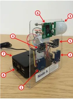
Fig. 2 shows the view of one of the four sensor nodes. Each sensor node is composed of six physical sensors (elements 1 to 6) connected to a Raspberry Pi minicomputer (element 7), which connects to the central processing unit by means of a USB wireless/WiFi adapter (element 8). The sensors included in each IoT node are as follows:
1) Momentary capacitive touch sensor based on the AT42QT1010 sensor (Adafruit 1374). This sensor provides a logical high output when touched by the user, and a logical low output otherwise. This sensor can be used to generate on/off patterns manually.
2) Toggle capacitive touch sensor based on the AT42QT1012 sensor (Adafruit 1375). This sensor alternates between high and low output states when touched by the user and can also be used to generate on/off patterns manually.
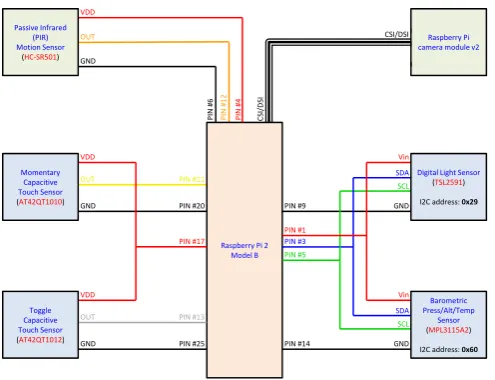
[image:3.595.43.294.57.205.2]VDD
GND
OUT
Raspberry Pi 2 Model B VDD GND OUT PIN #11 PIN #13 Vin GND SCL SDA Vin GND SCL SDA PIN #3 PIN #5 VDD GND
OUT Raspberry Pi camera module v2
CSI/DSI CSI /D SI P IN #4 P IN #6 P IN #1 2 Passive Infrared (PIR) Motion Sensor
(HC-SR501)
Momentary Capacitive Touch Sensor
(AT42QT1010)
Toggle Capacitive Touch Sensor
(AT42QT1012)
Barometric Press/Alt/Temp
Sensor
(MPL3115A2) I2C address: 0x60
Digital Light Sensor
(TSL2591) I2C address: 0x29
[image:4.595.43.291.53.243.2]PIN #1 PIN #9 PIN #14 PIN #20 PIN #25 PIN #17
Fig. 3. Connection of physical sensors to the Raspberry Pi 2 Model B.
4) Light sensor based on the TSL2591 sensor (Adafruit 1980). This high-range luminosity sensor contains both infrared and full-spectrum diodes that can provide illuminance measurements (in lux) of the infrared and full-spectrum light. Both values can be used to compute the illuminance in the human-visible spectrum (as the difference between both) and the corresponding luminosity perceived by the human eye (by means of an empirical formula). In practice, this physical sensor integrates four logical sensors.
5) Barometric pressure, altitude and temperature sensor based on the MPL3115A2 sensor (Adafruit 1893). This sensor contains a barometric pressure sensor that provides pressure measurements (in Pascals) and the equivalent altitude (in metres) along with temperature measurements (in Celsius).
6) Raspberry Pi camera module version 2, based on the Sony IMX219 8-megapixel image sensor. This mod-ule can provide 3280×2464 pixel static images and supports 1080p30, 720p60 and 640×480p90 video.
The six physical sensors are connected to a Raspberry Pi 2 Model B (element 7 in Fig. 2) as shown in Fig. 3. Except the camera module, which uses its own camera/display serial interface (CSI/DSI), the rest of sensors are connected via the general-purpose input/output (GPIO) pins. While sensors 1-3 provide simple logical binary (high/low) outputs and can be connected to standard logical input pins, sensors 4-5 are based on the I2C bus protocol and are therefore connected to the SDA/SCL pins. All sensors are powered from 3.3-volt pins so that the logical outputs provide a voltage compatible with that of the GPIO pins (i.e., 0 volts for logical low and 3.3 volts for logical high), except the motion sensor which requires at least 5 volts (but provides a 0/3.3-volt output). Table I shows the maximum current consumption of each sensor. Due to the limitations of the internal 3.3-volt voltage regulator of the Raspberry Pi, the GPIO pins can safely draw a maximum of 50 mA distributed across all 3.3-volt pins (including input, output, and 3.3-volt power pins). The maximum current consumption
TABLE I. MAXIMUM CURRENT CONSUMPTION OF EACH SENSOR.
Sensor Maximum (mA)
Momentary touch sensor (1) 2.03†
Toggle touch sensor (2) 1.67‡
Light sensor (4) 0.4§
Press. / alt. / temp. sensor (5) 2¶
Motion sensor (3) 65
Camera (6) 250
Fig. 4. View of the four IoT sensor nodes.
of the sensors connected to these pins (1, 2, 4 and 5) is around 6 mA, and the current through any individual pin does not exceed the 16 mA limit. The motion sensor is powered via a 5-volt pin and the camera module is powered via the CSI/DSI interface; for these two sensors there is no current limit other than that of the main power supply. The maximum current consumption of the Raspberry Pi 2 Model B board under stress conditions (including USB devices) is 820 mA1, which along with the camera module (250 mA), motion sensor (65 mA) and rest of sensors (6 mA), leads to a maximum consumption of 1141 mA per sensor node (2000 mA power supply is used).
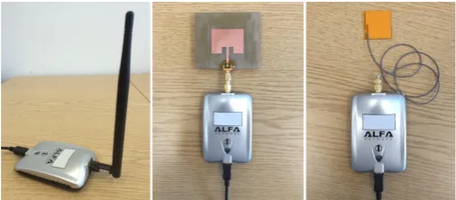
IoT sensor nodes are identical and implemented as detailed above (see Fig. 4). The connectivity between the IoT nodes and the central processing unit is accomplished by means of IEEE 802.11 wireless links. To this end, the IoT nodes and the central processing unit are equipped with 2.4 GHz USB wireless adapters Edimax EW-7811UN (element 8 in Fig. 2), which offer a wide range of configuration options for a fine tunning of the radio operation conditions. The prototype offers the possibility to employ other antennas by means of an external adapter (Alfa Network AWUS036H), which provides an SMA connector for external antennas. Fig. 5 shows the external adapter with different types of antennas. This feature is particularly appealing when evaluating a particular antenna design and its potential impact on other components of the system, both at the link and system level. For example, flexible antennas may be suitable for certain IoT devices (e.g., wearables) but their radiation pattern, directivity and other properties may be affected by the different positions to which they may be subjected, which may also have an impact on the quality of the wireless link (and interference patterns) and affect ultimately the data processed at the application layer.
1http://www.raspberrypi.org/help/faqs/#powerReqs
∗Obtained by interpolating the consumption values provided in the datasheet
(378.5µA@3V and 542.5µA@4V, i.e. 427.7µ[email protected]) and including the
current consumption of the LED (1.6mA).
†Obtained by interpolating the consumption values provided in the datasheet
(59µA@3V and 88µA@4V, i.e. 67.7µ[email protected]) and including the current
consumption of the LED (1.6mA).
‡Maximum current consumption when actively sensing.
[image:4.595.309.561.67.245.2]Fig. 5. External 2.4 GHz USB wireless adapter with different antenna designs: whip antenna (left), microstrip antenna (center), flexible PCB antenna (right).
B. Software Implementation
The IoT network can be configured in different ways in order to meet particular needs. Communication between the central processing unit and the IoT sensor nodes relies on Matlab features for remote access of Raspberry Pi computers, which is based on TCP/IP. This means that the IoT sensor nodes employed in the prototype could be virtually anywhere on the world and would be able to communicate with the cen-tral processing unit as long as they have a valid IP address. For convenience, the IoT network in the prototype is configured as a local ad-hoc network with private IP addresses where the central processing unit acts as an access point to which the IoT nodes are connected as terminals. This is a simple and convenient setup for experiments in a laboratory environment and moreover represents a realistic configuration since many future IoT devices are likely to be connected to the Internet via wireless access points or similar network infrastructures.
The central processing unit runs Microsoft Windows 7 op-erating system and employs theMicrosoft Virtual Wifi Miniport Adaptertechnology to provide connectivity as an access point to the IoT sensor nodes. This technology enables a physical wireless adapter to be virtualised into several logical adapters, which can be useful for example to access several WiFi networks with the same physical adapter or to share an Internet connection with other wireless devices. This technology is used here to configure the central processing unit as an access point to which the IoT sensor nodes can connect, thus enabling the direct communication among nodes in the IoT network.
The central processing unit is configured as an access point by running the following two commands (as administrator):
1) netsh wlan set hostednetwork mode=allow ssid=IoT-testbed key=eFutures
2) netsh wlan start hostednetwork
The first command configures the central processing unit as an access point hosting a network with name/service set identifier (SSID) IoT-testbed and access password eFutures. The second command starts the network. Once the hosted network has been started, any WiFi-equipped device will be able to connect to the network IoT-testbed (using the password eFutures) and communicate with other devices connected to the same network. This network is used to enable communication between the central processing unit and the IoT sensor nodes. For this to be possible, the IoT sensor nodes are configured to automatically search and connect to this
network at startup. This is easily accomplished by adding to the
file /etc/wpa_supplicant/wpa_supplicant.conf
of the Raspbian operating system running on the IoT sensor nodes the following lines:
network={
ssid="IoT-testbed" psk="eFutures" }
This information will be employed by the IoT sensor nodes to connect automatically to the IoT network hosted by the central processing unit at startup. By default, this network will use private IP addresses in the range192.168.137.0/24, where the default gateway IP address 192.168.137.1 is assigned to the central processing unit (since Window’s hosted network functionality is intended to share a computer’s Internet connection with other wireless devices) and the rest of network nodes (i.e., the IoT sensor nodes) are assigned random IP addresses by the central processing unit via Dynamic Host Configuration Protocol (DHCP). To facilitate the identification of the IoT nodes in the network, they are configured with pre-defined host names following the formatRBPi2-Node-X
where X can be A, B, C or D. Since a Windows hosted network will have by default a domain name mshome.net, the IoT sensor nodes can be accessed remotely by their complete host/domain nameRBPi2-Node-X.mshome.net
regardless of the IP address assigned by the central processing unit - the Domain Name System (DNS) protocol will translate each host/domain name to the corresponding IP address. This approach removes the need to configure and manage fixed IP addresses, which may lead to some issues for example when adding or removing nodes to the system.
Communication between the central processing unit and the IoT sensor nodes currently relies on Matlab functions for remote access of Raspberry Pi computers. This feature of Matlab simplifies the remote access to the IoT sensor nodes, however it has some limitations, in particular regarding the ability of the IoT nodes to initiate or trigger certain events and communications. While the current implementation based on Matlab’s communications features is sufficient for experimentation and proof-of-concept, future plans to extend the prototype include the implementation of communication protocols that remove the above mentioned limitations such as the Message Queuing Telemetry Transport (MQTT) pro-tocol. MQTT is an ISO standard (ISO/IEC PRF 20922) [16] messaging transport protocol based on a client-server publish-subscribe model that runs on top of TCP/IP and is light weight, open, simple, and designed to be easy to implement, which is particularly important in low-cost low-complexity IoT nodes where a small code footprint is required and/or network bandwidth may be limited. A variation aimed at embedded devices on non-TCP/IP networks, such as ZigBee, is available as well [17]. Other alternative protocols are Advanced Message Queuing Protocol (AMQP) [18, 19], Constrained Application Protocol (CoAP) [20], and Extensible Messaging and Presence Protocol (XMPP) [21–25].
possible to emulate other network topologies (e.g., forwarding a message from one IoT sensor node to another via the central processing unit), this is currently not needed and, as mentioned above, the current implementation is sufficient for experimen-tation and proof-of-concept. Nevertheless, the implemenexperimen-tation of communication protocols as the ones mentioned above may extend the prototype capabilities by enabling direct node-to-node links without involving the central processing unit.
Communication between the IoT sensor nodes and the central processing unit takes place via direct wireless links. In a real IoT network, certain fixed network infrastructure is likely to be present between both, which may result in packet delays and packet losses depending on the network congestion situation. A computer could be introduced in the prototype between the IoT sensor nodes and the central processing unit to capture TCP/IP packets sent by the IoT sensor nodes and selectively delay or discard some of them in order to reproduce network congestion situations. However, a simpler approach to achieve a similar effect is to selectively delay (in the central processing unit) the data reports from the IoT nodes before processing them, or discard them, according to a suitable packet delay/loss model [26, 27], which removes the need for an additional computer in the prototype.
The central processing unit first establishes a TCP/IP connection with each IoT sensor node. Once an individual network connection is established with each node, the central processing unit configures (for each node) the GPIO pins taking into account the connections shown in Fig. 3, creates an I2C connection with the light and pressure/altitude/temperature sensors based on their I2C addresses (see Fig. 3), configures the I2C sensors (in particular: the gain for the light sensor can be configured as low/1x, medium/25x, high/428x and maximum/9876x; the integration time of the light sensor can be configured from 100 ms for bright light to 600 ms for dim light in increments of 100 ms; and the oversampling ratio for the pressure/altitude/temperature sensor can be configured from 1 to 128, which leads to minimum time intervals between samples from 6 to 512 ms), and finally creates a connection with the cameras and configures their parameters (resolution, image quality, rotation, horizontal/vertical flip, frame rate, brightness, contrast, saturation, sharpness, exposure/exposure compensation modes, and image effects).
Once IoT sensor nodes are configured, the central process-ing unit can start gatherprocess-ing data from the sensors. Each sensor node can provide camera snapshots and videos in addition to the reading from a total of ten sensors, namely momen-tary touch sensor state, capacitive touch sensor state, motion detection state, illuminance (in lux) in the infrared/human-visible/full spectrums and human eye perception (based on an empirical formula), pressure (in Pascals), altitude (in metres), and temperature (in Celsius). Note that this represents a net-work with an effective total of 40 sensors (distributed among 4 sensor nodes) in addition to the picture/video sensors of each node. In order to emulate different scenarios that can be found in IoT networks, the prototype offers the possibility to gather data in the following ways:
• Synchronous full data reporting. In this mode of operation, the central processing unit collects data periodically from all sensors in all nodes. A config-urable data polling period determines the time interval
between two consecutive data polling events. In every data polling event, the central processing unit requests a reading from each of the 10 sensors installed in each of the 4 IoT sensor nodes. This mode of operation emulates an IoT network where all sensors provide periodic data reports in a synchronous way.
• Synchronous partial data reporting. This mode of operation is similar to the synchronous full data re-porting mode, with the exception that only a certain percentage (lower than 100%) of the sensors available in the network provide a data report in every periodic data polling event (if the percentage is configured as 100%, then this mode of operation is equivalent to the synchronous full data reporting mode). In this mode, the central processing unit computes first the number of sensors to be polled (i.e., the number of data polling events) based on the selected percentage of sensors and the total number of sensors available in the network. In each data polling event, one of the four IoT sensor nodes is selected randomly (by generating a random integer number from 1 to 4) and then one of the ten sensors available in that node is selected randomly (by generating a random integer number from 1 to 10). The process is repeated until the required number of sensors per data polling event is reached. This mode of operation emulates an IoT network where sensors provide periodic data reports in a synchronous way but not all sensors have new data to report in every data reporting event.
• Asynchronous data reporting.In this mode of opera-tion the time instants of the data reporting events are individually decided for each sensor available in the network based on a Poisson point process with an indi-vidually configurable interarrival time for each sensor, or another suitable model. The central processing unit checks constantly the polling time scheduled for each sensor in the network. When the polling time for a particular sensor is reached, the sensor is polled (i.e., a data report is provided by the sensor) and the next polling time is generated based on the corresponding Poisson point process or the employed model. This mode of operation emulates an IoT network where sensors provide data reports in an asynchronous way.
avoid interference and enable spectral coexistence with other existing radio communication systems (as explained in more detail in Section IV). These are just some examples of the type of experiments in the context of IoT enabled by the developed prototype. Detailed examples will be provided in Section VI.
The data collected from the sensors available in the net-work is processed in the central processing unit, where the intelligence is implemented, using Matlab. Matlab was selected given its comprehensive set of powerful and versatile functions that enable sophisticated data operations and simplifies the processing of complex data sets. Some illustrative examples on novel data processing methods evaluated with the developed prototype are provided in Section VI-A.
When an experiment is finished, the prototype is shut down by following two steps. First, the IoT sensor nodes are shut down remotely from the central processing unit by running the following command for each node:
start /B plink.exe -l pi -pw raspberry RBPi2-Node-X.mshome.net sudo poweroff
where X is replaced with A, B, C and D. This command uses Plink2 (a free and open-source command-line network connection tool) to shut down each node individually. Finally, the IoT network is stopped by running the command:
netsh wlan stop hostednetwork
which stops the hosted network in the central processing unit.
IV. COEXISTINGRADIOSUBSYSTEM
As mentioned in Section I, a significant amount of devices are expected to be connected to the IoT via wireless links using different types of radio access technologies such as IEEE 802.11 WLAN (WiFi) networks or mobile communication net-works. Forecasts of billions of IoT devices in the foreseeable future indicate that there will be a high demand for spectrum, however the frequency allocation charts of most countries are currently overcrowded. In this context, spectrum sharing approaches based on dynamic spectrum access and cognitive radio techniques are particularly promising in the context of IoT and the availability of adequate platforms to assess the performance of new spectrum access approaches is of great importance. The developed prototype includes a coexisting radio subsystem operating in the same frequency band as the IoT subsystem, i.e., the 2.4 GHz Industrial, Scientific and Medical (ISM) band. While the IoT subsystem is constrained to the IEEE 802.11 communication standard, the coexisting radio subsystem relies on a flexible design based on Software-Defined Radio (SDR) devices that can virtually implement any radio communication technology. This subsystem can be configured to coexist in an interference-free manner with the IoT subsystem or generate certain interference patterns. This subsystem extends significantly the range of experiments that can be conducted with the developed prototype by introducing a spectrum-sharing dimension and enabling the study of inter-actions of an IoT network with other communication systems as well as the analysis of the resulting impact at higher layers.
2http://www.chiark.greenend.org.uk/~sgtatham/putty/download.html
A. Hardware Implementation
The coexisting radio subsystem is composed of one trans-mitter and two receivers. The transtrans-mitter (receiver) is im-plemented with USRP B200 (B210) SDR devices, respec-tively (see Fig. 6). While the USRP B200 is equipped with one transceiver, the USRP B200 includes two transceivers, which enables the implementation and evaluation of diversity reception techniques at the receivers. Moreover, one of the USRP B210 units can be used as a transmitter in order to introduce Multiple-Input Multiple-Output (MIMO) techniques (the two USRP B210 channels can be used as two synchronised transmitters and/or receivers, thus enabling a full 2×2 MIMO system, or higher order if synchronised with other units).
In reception, USRP devices capture and amplify the radio-frequency signal received by the antennas (dual-band 2.4/5 GHzλ/2 whip antennas, model Mobilemark PSKN3-24/55S), performs down-conversion to a lower intermediate frequency at which the signal is sampled at a configurable sample rate up to 61.44 MS/s with a resolution of 12 bits, and decimates the samples to baseband before sending them (in complex I/Q format) to a host computer via a USB connection. A computer implementing the receiver in software captures and processes the signal samples. In transmission, the computer implements in software a transmitter that generates signal samples, which are interpolated by the USRP to the appropriate intermediate frequency, converted to the analog domain and up-converted to the radio-frequency for transmission. USB 3.0 connections allow up to 56 MHz of instantaneous bandwidth in SISO (1x1) mode and up to 30.72 MHz in MIMO (2x2) mode (USB 2.0 connections allow a maximum rate of 8 MS/s and an approximate maximum usable bandwidth of 7-8 MHz).
When experiments are conducted in an indoor environment (in particular inside the same room), transmission/reception power limitations should be observed to ensure that all devices operate under safe conditions. The USRP B200/B210 can transmit at a maximum output power of 20 dBm and tolerates a maximum input power of -15 dBm. The receiver might be damaged if placed too close to the transmitter. A radio propagation model suitable to the scenario of operation can be used to determine the minimum separation distance between transmitter and receivers. According to the indoor pathloss model of the recommendation ITU-R P.1238-8 [28], for a frequency of operation of 2400 MHz (lowest point and worst case of the 2.4 GHz ISM band), a power loss coefficient of 30 (office environment at 2.4 GHz), and devices operating in the same floor, a distance of 1 metre (minimum distance for which the model is valid) provides an atennuation of 40 dB, which is greater than the minimum 35 dB required to guarantee a safe operation at maximum transmission power.
B. Software Implementation
Fig. 6. Coexisting radio subsystem: Transmitter based on USRP B200 (left) and receivers based on USRP B210 (right).
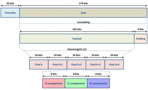
For proof-of-concept studies and demonstrations, the co-existing radio subsystem currently implements in Matlab a simple communication system designed for the transmission of a unidirectional and constant flow of data. Source data are interpreted as a sequence of bytes that are converted into bits for transmission using Quadrature Phase Shift Keying (QPSK) modulation. Data are transmitted in frames of 200 bits. The first 26 bits are header bits used for frame synchronisation at the receiver. The header bits are obtained by oversampling by two a 13-bit Barker code (i.e., repeating the Barker code bits twice), which ensures the transmission of the Barker code on both in-phase (I) and quadrature (Q) components of the QPSK-modulated signal. The remaining 174 bits are used for data transmission and can be configured in a flexible manner.
Fig. 7 shows an example of frame format for the transmis-sion of true-colour (24-bit) images (although the same format can be used or easily adapted for the transmission of any other type of data). A true-colour image with a height ofNh pixels and a width ofNwpixels can be represented as aNh×Nw×3 matrix containing three sub-matrices, each of which represents the corresponding values for the red (R), green (G), and blue (B) colour components for each pixel. Each pixel value is coded with 8 bits (numerical range from 0 to 255). Thus, the transmission of one pixel requires 24 bits. Each frame contains 5 consecutive pixels as shown in Fig. 7, which are read from the source image left-to-right and top-to-bottom. The 5 pixels (120 bits) are encoded with a Hamming(15,11) code to protect the information against transmission errors. This code has a rate of 11/15 ≈0.73 and outputs 165 bits, which constitutes the payload of the frame. The remaining 9 bits are padded with random bits. The payload and padding bits are scrambled over the data field of the frame using the generator polynomial
p(x−1) = 1 +x−1 +x−2 +x−4. The purpose of this is
twofold. First, transmission errors typically occur in bursts of consecutive bits and the effectiveness of error-correcting codes in general decreases when the erroneous bits are close to each other. The descrambling performed by the receiver spreads the erroneous bits, thus increasing the effectiveness of the employed error-correcting code. Secondly, scrambling guarantees a balanced distribution of zeros and ones, which facilitates the timing recovery at the receiver.
Frames are modulated using QPSK (with Gray mapping), up-sampled by a factor of 4, and filtered with a Square Root Raised Cosine (SRRC) filter (to minimise inter-symbol interference) with a roll-off factor of 0.5 and a span of 10 symbols (i.e., 40 samples). The filtered samples are sent to the
Preamble
Payload
Pixel k+1 Pixel k+2 Pixel k+3 26 bits
165 bits
24 bits 24 bits 24 bits 24 bits 24 bits
8 bits
G component
8 bits 8 bits
Padding 9 bits
R component B component
Pixel k Pixel k+4
Hamming(15,11) Data 174 bits
[image:8.595.40.293.54.164.2]Scrambling
Fig. 7. Link level frame format for the transmission of images.
USRP transmitter, which is configured to operate at a sample rate of 20 MS/s. Since this sample rate may be excessive for real-time operation with an average computer, the output of the SRRC filter is set at 200 kS/s and the samples are interpolated by a factor of 100. This leads to an effective data rate of 50·103 QPSK-modulated symbols per second (i.e., 100 kbps),
which can be increased for powerful computers by reducing the interpolation factor. The USRP transmitter operates at a configurable frequency within the 2.4 GHz ISM band, which can be selected (along with the transmission power) to generate specific interference patterns on the IoT subsystem.
In order to recover the original image, the receiver needs not only to revert the operations performed by the transmitter but also compensate the impairments of the wireless channel. To achieve this, the receiver includes Fast Fourier Transform (FFT)-based coarse frequency compensation, Phase-Locked Loop (PLL)-based fine frequency compensation, timing re-covery with fixed-rate re-sampling and bit stuffing/skipping, frame synchronisation, and phase ambiguity resolution (imple-mentation details are omitted for brevity, see [29] for details). Moreover, the receiver also needs to identify the beginning of a new image (i.e., the pixel on the top-left corner of the image). In order to facilitate this, the transmitter sends a predefined number of frames with the 120 bits of the message set to zero to indicate the beginning of a new image. The first non-zero framecorresponds to the first 5 pixels of the image. Note that this sequence of zeros is equivalent to 5 consecutive black pixels (the black colour is encoded as [0,0,0] in the RGB space). Therefore, an image with many black pixels may be incorrectly decoded at the receiver. To prevent this problem, all zero values in the original image are replaced with a value of 1 (the difference is not noticeable to the human eye).
Fig. 8. Spectrum monitoring subsystem.
V. SPECTRUMMONITORINGSUBSYSTEM
The purpose of the spectrum monitoring subsystem is to monitor and record (for off-line analysis) the spectral activity in the frequency band shared by the other two subsystems. This can be useful to understand how several systems and radio technologies coexist in the same frequency and identify particular interference patterns between systems. Spectrum analysers can provide relevant information such as effective channel occupied bandwidth, spectral masks, Received Sig-nal Strength (RSS), channel power measurements for several radio technologies, Adjacent Channel Power/Leakage Ratio (ACPR/ACLR), etc. It can also be employed to understand how different systems react to interference (e.g., moving to a different radio channel) or associate certain errors observed in one system at a particular time instant with interference from another system that was active at the same time instant.
This subsystem does not require a specific implementation since a standard spectrum analyser can be employed. Some of the illustrative results provided in Section VI were obtained using an Aaronia Spectran HF-60105 V4 X spectrum analyser (see Fig. 8) with the same antenna used by the transmitter and receivers of the coexisting radio subsystem (dual-band 2.4/5 GHz λ/2 whip antenna, model Mobilemark PSKN3-24/55S). This is a low-cost USB spectrum analyser and despite some limitations it is sufficient for the purposes of the prototype.
VI. ILLUSTRATIVEEXAMPLES
This section presents some examples illustrating the poten-tials and capabilities of the developed prototype in the study of future IoT systems. The developed prototype is flexible enough to embrace a wide variety of experiments in the context of IoT systems and the examples shown in this section are just a small subset of possible experiments. Other types of studies and experiments enabled by the developed prototype, although not shown here, are discussed in Section I.
A. Smart IoT data processing
As discussed in Section I, data sets in future IoT systems are expected to be so large and complex that traditional data processing approaches are deemed inadequate, thus claiming for innovative solutions to extract relevant and useful infor-mation. This first example shows how the prototype can be employed to explore new smart IoT data processing methods in order to extract meaningful information from the received data.
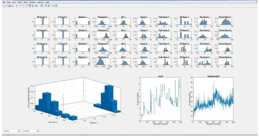
The implemented system effectively counts with a high number of sensors as discussed in Section III-B (40 sensors distributed among 4 sensor nodes in addition to the picture/video sensors of each node). Fig. 9 shows a screenshot of one of the several visualisation screens implemented in the central processing unit of the IoT subsystem. Each subfigure shows in real-time the history of measurements reported by each sensor node for a particular parameter (the last 20 measurements for each sensor are shown). This shows how a relatively low/moderate number of sensors can produce a significant amount of data and highlights the need and importance of developing adequate and efficient smart IoT data-processing methods.
In this illustrative example, a simple yet insightful method for data processing inspired by Information Theory is imple-mented. An important finding of Information Theory is that the more surprising a message is, the more information it contains [10, 11]. Therefore, in scenarios with high volumes of data, the value will not come from the volume of traffic but from finding unexpected or surprising new trends or events. Using the terminology from Information Theory, the amount of informationI carried by a messagexk from a set{xk}Kk=1
ofKmutually-exclusive messages is inversely proportional to its probability of occurrence P(xk)and can be defined as:
I(xk) = log2
1
P(xk)
(1)
wherek= 1, . . . , K, and PK
k=1P(xk) = 1. The base of the
logarithm in (1) determines the units ofI (bits for base 2).
Eq. (1) considers the case of a single source of information. The developed prototype implements multiple sensors, each of which can be seen as a source of information. In this context, (1) can be rewritten for convenience as:
I(xm,n) = log2
1
P(xm,n)
(2)
where the index m = 1, . . . , M identifies an individual sensor (M is the number of sensors in the system, i.e.,
M = 40 in the current prototype implementation), and the index n = 1, . . . , Nm identifies the message sent by the
mth sensor (Nm is the number of elements in the set of
possible messages{xm,n}Nm
n=1for themth sensor). In sensors
with discrete outputs (e.g., binary on/off sensors such as the touch and motion sensors) the application of this model is straightforward (e.g.,Nm = 2for binary sensors). In sensors with continuous outputs such as temperature and pressure, the likely range of output values for each sensor can be classified into a set ofNmbins with a bin width wmsuch that:
Nm=
max
n{xm,n} −minn{xm,n}
wm
(3)
A continuous output value xm is then classified into the nth bin ifxm∈[minn{xm,n}+ (n−1)wm,minn{xm,n}+nwm].
Fig. 9. Screenshot showing the real-time monitoring of all the available sensor data.
Consider initially the outputs xm1,n1 and xm2,n2 of two
sensors with indices m1 and m2, respectively. In this case a
joint surprisalparameter can be defined as:
Sjoint(m1, m2) = log2
1
P(xm1,n1, xm2,n2)
(4)
where P(xm1,n1, xm2,n2) is the joint probability of
simulta-neous occurrence of output xm1,n1 in sensor m1 and xm2,n2
in sensorm2. This definition can be extended to an arbitrarily
large set of sensors, leading to the more general definition:
Sjoint(M) = log2
1
P(xm1,n1, . . . , xm|M|,n|M|)
!
(5)
whereMis a predefined set of sensor indices and|M|is the cardinality (number of elements) of the set. This definition, however, can lead to practical implementation problems even for a relatively moderate number of sensors. In a practical implementation, the joint probability for M sensors can be characterised by anM-dimensional histogram whose elements can be computed based on the history of past outputs. If each sensor can output Nm different values, the histogram would need to storeQM
m=1Nmelements. For Nm=N ∀mthe size
of the M-dimensional histogram would be of NM elements.
This problem can be overcome by introducing the assumption of independent sensors, which would lead to the introduction
of anindependent surprisalparameter defined as:
Sindep(M) = log2
1
Q
m∈MP(xm,n)
(6)
When setM is selected as the set of all sensors available in the system (i.e.,M={1, . . . , M}), (6) can be expressed as:
Sindep(M) = log2
1
QM
m=1P(xm,n)
!
(7)
The implementation of this alternative definition only requires an individual one-dimensional histogram for each sensor, and the total number of elements to be estimated and stored reduces toPM
m=1Nm(onlyM N elements in the example above).
Fig. 10. Screenshot showing the real-time computation of sensor data histograms and the surprisal parameterS(M).
the number of considered sensors is low, otherwise (6) would be more convenient. If a small number of sensors is considered, then (5) may be used regardless of the data reporting mode.
Note that the probabilities in the denominators of (4)–(7) characterise the joint probability that the sensors inMoutput a particular set of values simultaneously. Those combinations of outputs that are more infrequent will have a lower joint probability and therefore the surprisal parameter S(M) will take a higher value. The variations in the value ofS(M)can be used to automatically identify and react to relevant events.
The ability of the proposed data processing method to detect relevant events was assessed with an experiment con-ducted in an office environment where a person was working on a computer. This represents a static scenario with sporadic movements of the worker around the office. The window was equipped with blinds to control the light intensity in the room.
Fig. 10 shows a screenshot of a visualisation screen im-plemented in the central processing unit to show the real-time computation of the sensor data histograms and both versions of the surprisal parameter. The small subfigures on the top half of the screen show the (individual one-dimensional) histograms of the data reported by the sensors (4 sensor nodes, 10 parameters per sensor). Every histogram is updated every time a new data report (value) is received (the last value is shown as a vertical red line in each histogram). The histograms of sensors with binary on/off outputs (three first columns of figures on the left-hand side) are composed ofNm = 2 bins (note that the touch sensors were not operated in this example) and the rest of sensors (with continuous outputs all of them) are discretised to Nm = 10 bins. All histograms are normalised
so that the value of every bin represents the probability of
receiving a message whose value falls within that bin. These probabilities are used to compute the independent surprisal parameterSindep(M)based on (6), where the setMis defined
as the set of all sensors providing a valid data report in the last data polling event (the IoT system operated in synchronous partial data reporting mode with about 60% of the sensors providing a data report in every data polling event). The time evolution of Sindep(M) is shown in Fig. 10 in the figure
labelled as Independent. Moreover, the joint 2-dimensional histogram/probability distribution of the motion sensor of node A and the visible light sensor of node C is computed (shown on the bottom-left corner of Fig. 10) and used to compute the joint surprisal parameterSjoint(M) based on (4)-(5). The
time evolution ofSjoint(M)is shown in Fig. 10 in the figure
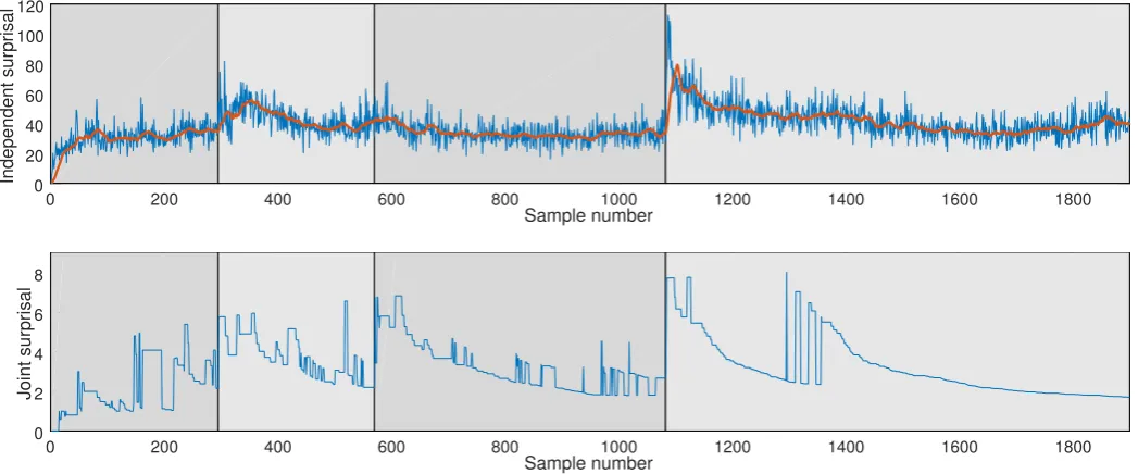
labelled as Joint. Fig. 11 shows a detailed view of how the surprisal parameters evolve over time in this experiment (the top figure also shows in red a moving-averaged version).
0 200 400 600 800 1000 1200 1400 1600 1800
Sample number
0 20 40 60 80 100 120
Independent surprisal
0 200 400 600 800 1000 1200 1400 1600 1800
Sample number
0 2 4 6 8
[image:12.595.42.566.55.273.2]Joint surprisal
Fig. 11. Time evolution of surprisal parameters.
fit reasonably well with the distribution of past values and therefore the independent surprisal parameter remains approxi-mately constant, with some peaks when movement occurs (this trend is better appreciated in the moving-averaged sequence). On the other hand, the joint surprisal parameter shows more drastic variations every time some movement is detected. The reason is that this version of the surprisal parameter depends on only two parameters/sensors and is therefore more sensitive to the variation of one of these parameters (moreover, a joint histogram needs more observations to be estimated accurately and the joint distribution is not well modelled at this point). The worker remains static most of the time during the first phase of the experiment, and when some movement is detected this represents an unusual event since it does not fill well with the distribution of past values. As a result, the surprisal parameter increases suddenly as soon as the movement occurs.
In the second phase of the experiment (sample numbers 295-570) the worker was moving constantly around the room (the blinds remained closed as in phase one). A similar pattern can be identified in both surprisal parameters. The value of the surprisal increases suddenly as soon as the worker starts mov-ing at the beginnmov-ing of phase two. This sudden increase occurs because the new measurements reported by the sensors do not fit well with the distribution of past measurements (when the worker was static) and as a result they are initially seen as unlikely events (because their corresponding probabilities in the histogram are low when they happen for the first time). When more similar measurements are reported by the sensors, the corresponding histograms are updated and their relative probabilities of occurrence increase, thus making them less unlikely and as a result the surprisal starts decreasing gradually. After certain time, this new situation becomes as frequent as the situation in phase one and the surprisal parameter decreases until it reaches a value similar/comparable to that of phase one.
In the third phase of the experiment (sample numbers 570-1083) the worker returns to the chair (with the blinds still closed), which is the same scenario as in phase one. One
might expect that this event would not be detected by the system since it would in principle be a situation the system is already familiar with. However, Fig. 11 clearly shows this is not the case since the system immediately detects the event via the increase of the surprisal parameter. In the case of the independent surprisal parameter, the increase is not very significant (probably due to the existence of similar sets of measurements in the histograms) but in any case it is notable enough to be detectable. In the case of the joint surprisal parameter it is interesting to note that the increase is actually very significant, which can be explained by the fact that the new sets of measurements received while the worker was moving resulted in a reshaping of the original histogram so that when the worker comes back to the original situation of phase one the reported measurements are not as likely as they used to be in the first phase of the experiment. In any case, after some time, the surprisal parameter decreases as the system becomes more familiar with the new situation.
Finally, in the last phase of the experiment (sample num-bers 1083-1900) the worker opens the blinds and returns again to a static position on the chair. As soon as the blinds open, the surprisal parameters increase suddenly and reach their highest peaks. This significant increase can be explained by the fact that this is the first time the system is exposed to a high light intensity and, even if the rest of parameters remain unaltered, the new values of light intensity reported by the sensors are so far from the distribution of past values that they are seen as very unexpected values and as a result the overall values of the surprisal parameters are affected. As in previous phases, as the system receives more measurements from the new scenario, the situation becomes less unlikely and the surprisal parameter decreases gradually (the peaks observed in sample numbers 1300-1400 were caused by the movement of some clouds, which led to some alternated periods of light/darkness).
2430 2437 2440 2446 2450 2457 2460 2465 2468 Frequency (MHz)
-100 -90 -80 -70 -60
Power (dBm)
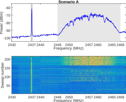
Scenario A
2430 2437 2440 2446 2450 2457 2460 2465 2468
Frequency (MHz) 50
100 150 200
[image:13.595.313.564.53.257.2]Sweep number
Fig. 12. Coexistence Scenario A (without inter-system interference).
world and react to them. The system keeps an updated version of the histogram of the values reported individually by each sensor and this information is exploited to determine how likely or unlikely a new set of data reports is. When an unexpected event occurs, the measurements reported by the sensors lead to a set of values with a low probability of occurrence and this helps the system identify such event and take actions automatically. The proposed method could be extended with features such as processing of surprisal values to determine what events are more relevant and should trigger a reaction from the system, which is proposed as future work.
The proposed method, while based on rather simple princi-ples, paves the way for the development of more sophisticated methods exploiting the full potentials of advanced fields such as data mining, artificial intelligence, or machine learning, among others. While the example shown in this section has not made use of the camera sensors, they can also be exploited in more sophisticated methods. For example the images captured by the sensors can be processed forego-motiondetection (i.e., the motion and rotation of the camera axes), which can be useful in applications where the sensors are worn or mounted on something that moves, the detection of people in front of the camera (in this case the camera would behave as an on/off sensor for the detection of human beings or objects), the identification of the type of environment (indoor, outdoor, urban, rural, etc.), or the extraction of descriptors that encode properties of the images as a whole. The range of possibilities is virtually unlimited and the developed prototype provides a suitable and flexible tool for a realistic evaluation of such innovative solutions in the context of IoT systems.
The illustrative example discussed in this section not only demonstrates that it is possible to design smart data processing methods to extract meaningful information from large volumes of data and effectively detect relevant events in the context of IoT systems, but also shows the ability of the developed prototype to implement and evaluate such type of methods under configurable and controllable realistic scenarios.
2430 2435 2440 2446 2450 2457 2460 2465 2468
Frequency (MHz) -100
-90 -80 -70 -60 -50
Power (dBm)
Scenario B
2430 2435 2440 2446 2450 2457 2460 2465 2468
Frequency (MHz) 20
40 60 80 100 120
[image:13.595.43.292.54.256.2]Sweep number
Fig. 13. Coexistence Scenario B (with inter-system interference).
B. Radio coexistence
In the example presented in Section VI-A the IoT sub-system operated without interference from other sub-systems (i.e., the coexisting radio subsystem was deactivated). This section presents an example where the IoT subsystem coexists with the coexisting radio subsystem (and other radio systems) in the same frequency band. The spectrum monitoring subsystem is used to monitor and record the spectral activity of both systems in the selected band of operation (the 2.4 GHz ISM band).
Two different coexistence scenarios are considered in this experiment, which are illustrated in Figs. 12 and 13 (these figures were obtained with the spectrum monitoring subsys-tem). In both scenarios the IoT subsystem operates in channel 10 of the 2.4 GHz ISM band as defined by the IEEE 802.11 standard (2446-2468 MHz) and its operation can be divided into three phases. In the first phase (approximately the first third of sweeps shown in Figs. 12 and 13) the IoT network is established but the IoT subsystem remains inactive. In this phase there is no communication between the IoT nodes and the central processing unit, and therefore there is no spectral activity, except for the beacon signals that the central processing unit transmits periodically (some of which are captured by the spectrum monitoring subsystem). In the second phase (approximately the second third of sweeps) the IoT subsystem is active and operates in synchronous partial data reporting mode, with around 60% of the sensors sending data reports in every data polling event, which results in some intermittent usage of channel 10. In the third and final phase of the experiment (approximately the last third of sweeps) one of the IoT nodes sends video with a resolution of 1920×1080 pixels at 30 frames per second in real-time, which requires a high data rate, thus forcing an intensive (constant) usage of channel 10 as it can be appreciated in Figs. 12 and 13.
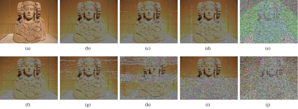
(a) (b) (c) (d) (e)
[image:14.595.47.557.54.241.2](f) (g) (h) (i) (j)
Fig. 14. Image transmitted and received by the coexisting radio subsystem under various operation conditions.
the coexisting radio subsystem operates at 2457 MHz (i.e., the center frequency of channel 10). Therefore, in scenario A there is no interference between both radio systems, while in scenario B the interference is maximum. The coexisting radio subsystem transmits an image file in a cyclic loop, thus resembling the transmission of a video, with the exception that the transmitted image is always the same, which allows a more accurate evaluation of the impact of interference on the system performance. The coexisting radio subsystem implements the physical layer features required for the successful transmission of data based on a QPSK modulation (as detailed in Section IV-B) but does not implement any interference prevention or interference management techniques thus making it very vulnerable to interference, as opposed to the IoT subsystem, which is based on IEEE 802.11 links and therefore counts with sophisticated methods to avoid and react to packet collisions.
This setup allows a detailed evaluation of the impact that the interference from an IoT system could have on other systems operating in the same frequency band, not only at the physical layer (e.g., bit, symbol or frame rates) but also at the application layer (e.g., visual quality of the received image).
During the experiment, the IoT subsystem did not appear to be affected by interference, at least to a significant extent. The data reported by all sensors were correct at all times. Only during some periods of interference the reception of data reports from the sensors experienced a noticeable delay (proba-bly because of packet collisions), and only in one occasion the connectivity was lost during a moment of high interference but was recovered some time later. On the other hand, the impact of interference on the coexisting radio subsystem, which does not implement mechanisms as sophisticated as those included in the 802.11 standard, was much more noticeable.
Fig. 14 illustrates the impact of interference on the co-existing radio subsystem. Fig. 14(a) shows the transmitted image and the rest of figures show the image received under different operation conditions. Fig. 14(b) shows the image received in Scenario A when the overall activity in the 2.4 GHz ISM band was extremely low and there was virtually no interference from any other systems. Although the image does not show any noticeable artefacts, it is slightly darker than the
original image, which could be explained by the transmission-reception process (in particular the up/down-sampling along with the use of SRRC filters). Figs. 14(c) and 14(d) show two images received in Scenario A with the IoT subsystem deactivated (first phase). Both figures show some lines with different numbers of consecutive incorrect pixels correspond-ing to frames received in error as a result of interference. Recall that pixels are transmitted from left-to-right and top-to-bottom, therefore interference leads to horizontal lines of consecutive erroneous pixels and the length of the line is proportional to the duration of the interference. Since the IoT subsystem was operating at a different frequency and with no ongoing communications, this interference was caused by other systems. While the interference pattern observed in Fig. 14(c) is rather irregular, the pattern in Fig. 14(d) appears to indicate that the interference was caused by a frequency hopping system, since interference intervals are observed at periodic time instants (when the interfering system hops to a frequency that overlaps with that of the coexisting radio subsystem) and with very similar durations (proportional to the time interval that the frequency hopping system remains in the same frequency). Since the coexisting radio subsystem and the IoT subsystem operate in different channels in Scenario A, one may expect they could never interfere with each other in such scenario. However this is not necessarily true. As a matter of fact, the image shown in Fig. 14(e), which corresponds to the third phase of the experiment (IoT subsystem transmitting video), indicates that the coexisting radio subsystem was severely affected by out-of-band emissions, or possibly by an increased noise floor, resulting from the transmission power of the IoT subsystem (17±1.5 dBm at maximum power).