Stability Boundary Analysis in Single-Phase
Grid-Connected Inverters with PLL by LTP Theory
Valerio Salis,
Student Member, IEEE,
Alessandro Costabeber,
Member, IEEE,
Stephen M. Cox,
Pericle Zanchetta,
Senior Member, IEEE,
and Andrea Formentini,
Member, IEEE
Abstract—Stability analysis of power converters in AC net-works is complex due to the non-linear nature of the conversion systems. Whereas interactions of converters in DC networks can be studied by linearising about the operating point, the extension of the same approach to AC systems poses serious challenges, especially for single-phase or unbalanced three-phase systems. A general method for stability analysis of power converters suitable for single-phase or unbalanced AC networks is presented in this paper, based on Linear Time Periodic (LTP) theory. A single-phase grid-connected inverter with PLL is considered as case study. It is demonstrated that the stability boundaries can be precisely evaluated by the proposed method, despite the non-linearity introduced by the PLL. Simulation and experimental results from a 10kW laboratory prototype are provided to confirm the effectiveness of the proposed analysis.
Index Terms—Linear Time Periodic Systems, Harmonic State Space Model, Stability Analysis, Power Converters, PLL
I. INTRODUCTION
A
C power systems based on power converters are complex and highly non-linear because both converters and loads often show a non-linear behaviour. Several practical cases of instability issues in such systems are discussed in the literature. For example, [1] reports an incident occurring on the Swiss railway power network due to the high level of harmonics generated by the interaction of new generation locomotive inverters. A more comprehensive review of potential instabil-ities affecting different railway systems is presented in [2]. In [3] it is stated that similar instability issues also affect LCC HVDC converters. Finally, [4] and [5] discuss several harmonic-related interactions, like the harmonics generated by the connection of wind and solar sources to the AC grid, causing resonances at low frequencies and leading to voltage and current distortions.Based on these examples, it follows that a theory for stability analysis of such systems is required. Existing analysis techniques can be broadly categorized into frequency and time-domain methods. When a balanced and symmetric three-phase AC system is considered, the analysis can be performed in the dq reference frame [6], but this is no longer the
This paper is an extension of a conference paper (Stability analysis of single-phase grid-feeding inverters with PLL using Harmonic Linearisation and Linear Time Periodic (LTP) theory) presented at COMPEL, 27-30 June 2016, IEEE 17th Workshop on.
V. Salis, A. Costabeber, P. Zanchetta and A. Formentini are with the Depart-ment of Electrical and Electronic Engineering, University of Nottingham, Not-tingham NG7 2RD, U.K. (e-mail: [email protected]; [email protected]; [email protected]; [email protected]).
S. M. Cox is with the School of Mathematical Sciences, University of Nottingham, Nottingham NG7 2RD, U.K. (e-mail: [email protected])
Manuscript received ****, 2016; revised ****, 2016.
case for unbalanced or single-phase systems. In such cases, one of the most popular frequency-domain method is the small-signal impedance-based stability criterion applied to the analysis of grid-connected power converters in the abc
frame, [7]. The system is equivalently represented as a source and a load subsystem. Each system is described by its own small-signal impedances, which is calculated using Harmonic Linearisation techniques as shown in detail in [8], [9], [10]. Finally, stability of the system is assessed by applying the Nyquist criterion to the ratio of load to source small-signal impedances. However, potential limitations might affect this method, as discussed in [11], especially in the case where instabilities occur at frequencies below the fundamental grid frequency. An extension of this method is reported in [12], where a two-dimensional admittance for single-phase voltage source converters is calculated, able to capture the frequency interactions between load and source subsystem up to twice the line frequency, possibly overcoming the aforementioned limitations. However, if higher harmonic couplings are to be considered, the complex maths behind this method might be a limitation.
Another frequency-domain method is the dynamic phasor approach [13], where the 2-dimensional source and load impedances are evaluated and the system stability is assessed using the Generalised Nyquist Criterion [14]. This analysis relies on the assumption that all the signals in the system have a dominant first harmonic component, such that the DC and the higher components are neglected. This might be a limitation for the analysis of systems where the second or higher order harmonics play an important role.
grid-connected converter in [19] and a general method for modelling linear and switching subsystems in [20]. Second, based on a HSS model, stability analysis can be performed. In [21] and [22] stability analysis is performed on a single-phase grid-connected converter in the continuous time-domain, and in [23] the analysis is carried out in the discrete time-domain based on linearised models of the system, but non-linearities due to the PLL are not included in the analysis. In [24] the non-linear dynamics introduced by the PLL is included in the analysis using a small-signal model and an impedance-based stability analysis is performed but precise stability boundaries are not provided. In [25] a rigorous method based on eigenvalue analysis and LTP theory is presented, however the digital computation delay, ZOH and PWM dynamics are not included and experimental results are not provided.
In this paper, the time-domain approach based on the HSS model of a grid connected single-inverter with PLL and DC bus represented by an equivalent DC source is investigated in detail. To provide a comprehensive evaluation of the proposed method, the analysis is performed both in the continuous and in the discrete time-domain, leading in both cases to accurate results. It is worth mentioning that the primary objective of the analysis is to highlight the impact of non-linearities, i.e. the PLL, on system stability. Therefore, high frequency modelling is out of the scope of this work. Nevertheless, computation delay and sampling and hold have been included in the analysis for completeness. Starting from the non-linear average state space model, linearisation is applied in order to derive a linearised model, obtaining an LTP system. Then LTP theory is applied and stability analysis is performed based on the eigenvalue loci of the system. This paper demonstrates that, if properly applied, the method allows an accurate identification of the stability boundaries of the system, i.e. the stability threshold where the system moves from stable to unstable operation. To limit the complexity of the discussion, the stability threshold is analysed as the amplitude of the current injected in the AC grid, Iref, increases. This simple choice has been made in order to highlight an instability effect that a simpler low-frequency linearisation approach for the PLL, used in conjunction with standard LTI stability analysis techniques, would not be able to identify. In fact, stability of a small-signal LTI model is independent of the amplitude of the control references. Even though previous literature exists on LTP theory applied to power converters, this work shows how the potential of the method can be exploited, guiding the reader through the theoretical procedure for stability analysis and quantifying the accuracy of the method. The paper is organized as follows: Section II provides a description of the system; Section III presents the continuous-time LTP stability analysis and Section IV the discrete-time one; in Section V analytical, simulation and experimental results for a 10kW
laboratory prototype are presented for different values of the grid inductor and of the damping resistor, showing in all cases good agreement with the expected stability boundaries; in Sections VI a comparison between continuous LTP and discrete LTP is provided.
II. SINGLE-PHASEGRID-CONNECTEDINVERTER WITH
PLL MODEL
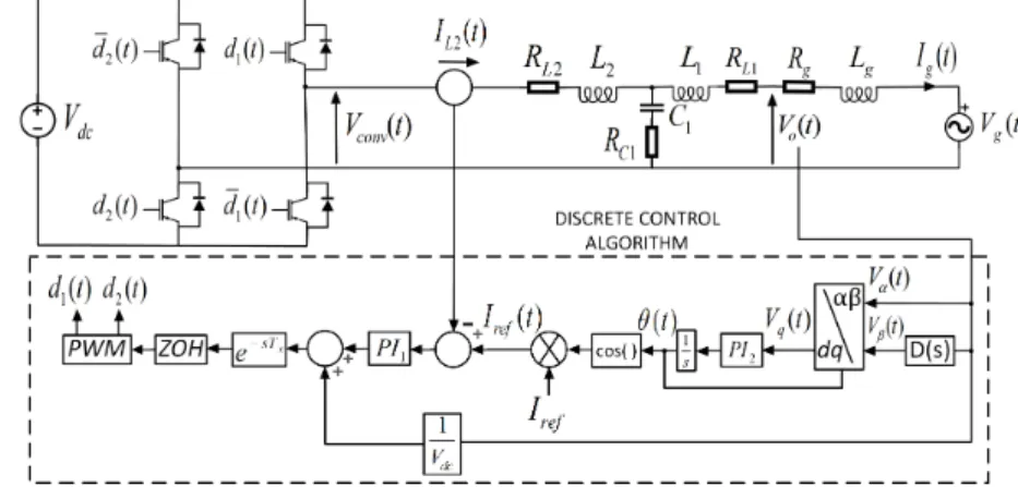
The system under study is a current controlled grid-connected inverter with PLL, as shown in Fig. 1. The single-phase inverter is supplied by a DC source, Vdc, and its output is connected through an L2C1L1 low-pass filter to
the grid, which in turn is represented by an ideal sinusoidal voltage source, Vg(t) =Vgsin(ωgt), in series with an RgLg impedance. Unity power factor operation is considered. A Phase Locked Loop (PLL) is used to measure the phase of the grid voltage and to generate the current reference signal,
Iref, for the inverter output current,IL2(t). A PI controller is
then used to control the inverter.
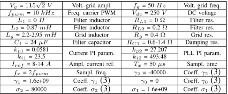
TABLE I:Continuous-time system parameters
Vg=115
√
2V Volt. grid ampl. fg= 50Hz Volt. grid freq.
fpwm= 10kHz Freq. carrier PWM Vdc= 250V DC voltage
L1= 0H Filter inductor RL1= 0Ω Filter res.
L2= 0.87mH Filter inductor RL2= 0.2Ω Filter res.
Lg= 2.2-2.95mH Grid inductor Rg= 0.4Ω Grid res.
C1= 24µF Filter capacitor RC1= 0.6-1.4Ω Damping res.
kp1= 0.0581 Current PI param. kp2= 27.207 PLL PI param.
ki1= 23.5 ki2= 493.48
Iref = 8-14A Ampl. current ref. Tx= 50µs Sampl. time
fx= 2fpwm Sampl. freq. γ2= -40000 Coeff.γ2(3)
γ1= 1.6e+09 Coeff.γ1(3) γ0= 0 Coeff.γ0(3)
σ2= 80000 Coeff.σ2(3) σ1= 1.6e+09 Coeff.σ1(3)
It will be shown that the parameterIref, which is related to the amount of power that the inverter injects into the grid, has a threshold value, above which the system becomes unstable. That is, the instability is due to the fact that the PLL is no longer able to generate the correct phase reference for the controller. It is worth noticing that a damping resistor Rc is used in the low-pass filter in order to simplify the design of the current control and focus on the analysis and quantification of the instability caused by the PLL.
For single-phase applications, the PLL needs to estimate the in-quadrature component of the grid voltage, Vo(t), and among the several available options a linear filter that in-troduces a Tg/4 delay at ωg is used in this paper: D(s) =
ωg2/(s2 +sωg +ωg2). In Fig.1 the controllers are assumed to be implemented in the continuous-time domain, but the actual experimental converter has a digital controller. In the continuous-time analysis, in order to accurately reflect the characteristics of the digital control while maintaining the lower complexity of a continuous-time system for stability analysis, the computation delay (Tx) with the zero-order hold (ZOH) delay of the pulse width modulator (PWM), (0.5
Fig. 1. Single-phase grid-connected inverter with PLL - switching model
analysis is based on the parameters that will later be used for the experimental prototype, summarised in Table I.
III. CONTINUOUSTIME-DOMAINANALYSIS
A. Continuous Non-Linear Time Periodic Average Model
The proposed analysis is based on the average model of the system. Since the main focus of the analysis is the instability caused by the incorrect behaviour of the PLL and it is known that such instability arises at frequencies far below that of the switching [24], the switching model is replaced by the average one and the analysis is performed on the latter. The unit computation delay, the ZOH and the PWM blocks are represented in the continuous time domain by the following transfer function:
H(s) =e−sTx1−e−sTx/(sT
x) (1)
The complex exponential is replaced with a first-order Pad´e approximation:
e−sTx= (n
1s+n0)/(d1s+d0) (2)
Substituting (2) in (1) gives the transfer function:
H(s) = (γ2s2+γ1s+γ0)/(s3+σ2s2+σ1s) (3)
which relates the output of the current controller to the duty cycle. The whole system is equivalently represented by the state-space model (4), which is an11thorder Continuous Non-Linear Time Periodic (NLTP) system, with all the state-space variablesTg-periodic and the non-linearity due to the presence of the PLL. The state-space variables x1(t)-x4(t) describe the internal dynamics of the PLL; x5(t) is the state-space variable associated to the current control PI; x6(t)represents the grid current, Ig(t); x7(t) the inductor current, IL2(t); x8(t)the voltage across the capacitor;x9(t)-x11(t)the internal dynamics of the computation delay, ZOH and PWM. The only input signal of the state-space model is the input voltageVg(t).
Vo(t) =(L1Rg−Lg(RC1+RL1))x6(t) +LgRC1x7(t)
+Lgx8(t) +L1Vg(t)
/(Lg+L1)
Vconv(t) =Vdcγ0x9(t) +Vdcγ1x10(t) +Vdcγ2x11(t)
˙
x1(t) =x2(t)
˙
x2(t) =−ωg2x1(t)−ωgx2(t) +ωg2Vo(t)
˙
x3(t) =x4(t)−kp2sin(x3(t))Vo(t) +kp2cos(x3(t))x1(t)
˙
x4(t) =−ki2sin(x3(t))Vo(t) +ki2cos(x3(t))x1(t) ˙
x5(t) =Irefcos(x3(t))−x7(t)
˙
x6(t) =−(RC1+RL1+Rg)x6(t) +RC1x7(t) +x8(t)
−Vg(t)
/(Lg+L1)
˙
x7(t) =
RC1x6(t)−(RC1+RL2)x7(t)−x8(t) +Vconv(t)
/(L2)
˙
x8(t) =
−x6(t) +x7(t)
/(C1) ˙
x9(t) =x10(t), x˙10(t) =x11(t)
˙
x11(t) =−σ1x10(t)−σ2x11(t) +ki1x5(t)
+kp1Irefcos(x3(t))−kp1x7(t) +Vo(t)/Vdc (4)
B. Review of Continuous Linear Time Periodic Systems Theory
Average models of real AC systems are usually NLTP, as shown in (4). Therefore, the first step is to linearise the system about its steady-state operating trajectory, reducing it to an LTP system for small perturbations, in contrast to DC systems where linearisation is applied about a constant steady-state operating point. Given a general Continuous NLTP system which isT-periodic:
˙
x(t) =f(x(t)) +g(x(t))u(t), y(t) =h(x(t)) +l(x(t))u(t)
(5) and given a steady-state input u¯(t), this system is solved numerically (in Matlab for example) and the steady-state solution, x¯(t), is obtained. Now linearisation is performed, so a small-signal perturbation is added to each input, output and state, i.e. u(t) = ¯u(t) + ˜u(t), y(t) = ¯y(t) + ˜y(t) and
x(t) = ¯x(t) + ˜x(t). These are substituted into (5) and taking into account only the perturbation terms gives the linearised model, which results in a Continuous LTP system:
˙˜
x(t) =A(t)˜x(t) +B(t)˜u(t), y˜(t) =C(t)˜x(t) +D(t)˜u(t)
both input and output spaces are the same and they include the same set of harmonic components. Thus:
q(t) =ejΩt +∞
X
n=−∞
qnejnωTt forq=u, x, y (7)
˙ x(t) =
+∞
X
n=−∞
(jΩ +jnωT)xnej(Ω+nωT)t (8)
By substituting (7)-(8) in (6), expanding the matrices A(t),
B(t),C(t)and D(t)in Fourier series and using the Cauchy product theorem, it is possible to write:
(jΩ +jnωT)xn =
∞
X
m=−∞
An−mxm+
∞
X
m=−∞
Bn−mum
yn =
∞
X
m=−∞
Cn−mxm+
∞
X
m=−∞
Dn−mum (9)
This is a concise representation of the input-output relationship between the Fourier coefficients of the input and output sig-nals. However, the manipulation of Fourier series usually leads to complicated calculation and for this reason the Toeplitz transform is introduced to simplify the analysis.
A Toeplitz transformation is defined as follows:
T[A(t)] =A=
. .. ... ... ... · · · A0 A−1 A−2 · · · · · · A1 A0 A−1 · · · · · · A2 A1 A0 · · ·
..
. ... ... . ..
(10)
which is a doubly infinite block Toeplitz matrix and the matrices Ai are the Fourier matrix coefficients of the T -periodic matrix A(t). A similar definition applies to the matrices T[B(t)] = B, T[C(t)] = C, T[D(t)] = D and to the vectors T[x(t)] = X, T[u(t)] = U, T[y(t)] = Y. Consider now the system of equations (9), which apply for all
n. The Toeplitz transform is used in order to obtain a clearer and more compact notation. Thus the Harmonic State Space Model (HSSM) of the LTP system that follows from (6) is as follows:
sX = (A − N)X+BU , Y=CX +DU (11)
withN =diag(. . . , N−n, . . . , N−1, N0, N1, . . . , Nn, . . .)and
Nn a diagonal matrix of the same dimensions as An with diagonal coefficients equal to jnωT. Through simple steps similar to the analysis of LTI systems, the Harmonic Transfer Function (HTF) of the system then follows from (11):
Y= ˆG(s)U , Gˆ(s) =C[sI −(A − N)]−1B+D (12)
Stability analysis can now be performed evaluating the eigenvalues of the matrix(A − N). If all the eigenvalues have
Re[λi] ≤ 0, where those with Re[λi] = 0 have algebraic multiplicity equal to 1, then the system is stable, otherwise the system is unstable.
So far an infinite number of coefficients has been considered in the Fourier series expansion. In the practical implementation of the analysis, a truncation order N is introduced, which
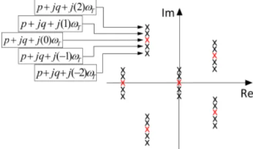
Fig. 2. General eigenvalue loci of an LTP system: red - important eigenvalues; black - translated copies
refers to the maximum harmonic number taken into account. If N = 2, for example, this means that the DC-component and the first and second harmonics are considered. The corre-sponding Fourier expansion involves the Fourier coefficients for n=−2,−1,0,1,2:
A(t) =
N X
n=−N
AnejnωTt=
2
X
n=−2
AnejnωTt (13)
and the following associated truncated Toeplitz form is con-sidered:
T[A(t)] =A=
A0 A−1 A−2 Z Z A1 A0 A−1 A−2 Z A2 A1 A0 A−1 A−2
Z A2 A1 A0 A−1
Z Z A2 A1 A0
(14)
withZ being a zero matrix of the same dimension as theAn. So when the truncation order is increased a larger number of Fourier coefficients of the Fourier expansion is taken into account and at the same time the dimension of the associated Toeplitz form increases. Thus, given an LTP system of order
p, i.e. with pstate-space variables, and a truncation orderN, the number of eigenvalues associated with the matrixA − N will be (2N+ 1)×p. However, onlypof these eigenvalues are relevant for stability analysis; all the others are translated copies of the original ones, with translation equal to jnωT,
n=±1, . . . ,±N. Fig. 2 shows an example of LTP pole loci withq= 6andN = 2. In red are depicted the important poles and in black their translated copies. It can be observed that for a large truncation order the eigenvalue loci result in long vertical lines of eigenvalues.
C. Continuous Steady-State Solution
As anticipated in the previous section, in order to apply linearisation the steady-state solutions of the system (4) must first be evaluated. We will discuss some mathematical consid-erations and then solve numerically the system of equations, exploiting the Harmonic Balance approach. It is worth men-tioning that the detailed derivation is provided for rigour and completeness. An approximated steady-state solution might be used in practice to reduce the analytical burden. Knowing that the converter is operating in an AC system, the set of steady-state solutions will be of the form:
¯
for i= 1,2,5,6,7,8,9,10,11; x¯3(t) =ωgt+ ¯x03 (15)
¯
x4(t) =to be defined ;V¯x(t) = V¯x
cos(ωgt+ arg( ¯Vx))
= ( ¯Vxejωgt+c.c.)/2, x=o, conv, g (16)
where c.c. stands for the complex conjugate of the term preceding it within the square brackets. Substituting these expressions in the non-linear state-space model gives us:
¯
x5= (Irefej¯x03−x¯7)/(jωg) (17)
¯
x6= RC1x7¯ + ¯x8+jVg RC1+RL1+Rg+jωg(Lg+L1)
(18)
¯
x7= RC1x6¯ −x8¯ + ¯Vconv RC1+RL2+jωgL2
(19)
¯
x8= (−x6¯ + ¯x7)/(jωgC1) (20)
¯
x9= ¯x10/(jωg) (21)
¯
x10= ¯x11/(jωg) (22)
¯ x11=
−σ1x¯10−σ2x¯11+ki1x¯5+kp1Irefej¯x03
−kp1x7¯ + ¯Vo/Vdc/(jωg) (23)
¯ Vo=
(L1Rg−Lg(RC1+RL1))¯x6+ (LgRC1)¯x7 +Lgx8¯ +L1Vg/j/(Lg+L1) (24)
¯
Vconv=Vdcγ0x¯9+Vdcγ1x¯10+Vdcγ2x¯11 (25)
These nine equations can now be solved numerically and the steady state solutions x¯5,x¯6,x¯7,x¯8,x¯9,x¯10,x¯11,V¯o,V¯conv obtained. Proceeding with the analysis gives:
¯
x2=jωgx¯1 , ¯x1=−jV¯o (26)
So the solutions x¯1,x¯2 are given by:
¯ x1(t) =
V¯o
cos(ωgt+ V¯o−π/2) (27)
¯
x2(t) =ωg V¯o
cos(ωgt+ V¯o) (28)
The last two quantities to be defined are x¯3 andx¯4:
¯
x3(t) =ωgt+ ¯x03 (29)
Hence:
˙¯
x3(t) =ωg= ¯x4(t)
−kp2sin(ωgt+ ¯x03) V¯o
cos(ωgt+ V¯o)
+kp2cos(ωgt+ ¯x03) V¯o
sin(ωgt+ V¯o) (30) Applying trigonometric simplification gives us:
¯
x4(t) =ωg−kp2sin( ¯Vo−x03¯ ) (31)
So it follows thatx4˙¯ (t) = 0. But from the state-space model, again using trigonometric simplifications, we have:
˙¯
x4(t) =ki2
−sin(¯x3(t)) ¯Vo(t) + cos(¯x3(t))¯x1(t)
(32)
And so:
˙¯
x4(t) =−ki2|V¯o|sin( ¯Vo−x03¯ ) (33)
which implies: V¯o−x03¯ = 0or±π. In our case, V¯o= ¯x03, which gives the last two solutions:
¯
x3(t) =ωgt+ V¯o , x4¯ (t) =ωg (34)
The steady-state periodic functions calculated in this subsec-tions will now be used to derive the continuous LTP model of the system.
D. Continuous Linearised Model
Following the steps illustrated in the previous section, the Continuous LTP small-signal model (35) for perturbations to the steady-state operating point of the Continuous NLTP system (4) is derived, which is of the form x˙˜(t) =A(t)˜x(t), withA(t)being a Tg-periodic matrix. In this particular case the only matrix coefficients of the Fourier series expansion which differ from zero areA0,A1andA−1; these are reported
in (36), (37) withA−1=A∗1 (*=complex conjugate). This is
due to the fact that the steady-state solutions for all the state variables are either DC or single-frequency Tg-periodic AC. It is now possible to derive the Toeplitz formAand evaluate the eigenvalues ofA − N to determine whether the system is stable or not. The full derivation is not reported for the sake of brevity.
IV. DISCRETETIME-DOMAINANALYSIS
A. Discrete Non-Linear Time Periodic Average Model
The stability analysis proposed in the previous Section is based on a simplified continuous-time model of the system. Another possibility is to perform the analysis based on a discrete-time model of the system, thus providing a direct representation of the digital implementation of the controllers in the DSP of the experimental set-up. However, from a stability point of view, both continuous and discrete-time approaches lead to an accurate identification of the stability boundaries, as it will be shown in Section V. First, the control algorithm implemented in the DSP is reported, which involves the discretization of the four continuous time blocks, i.e. current controller, linear filter for quadrature signal generation, PLL controller and integrator block. TheZOHtransformation is applied to the PI controller and to the integrator of the PLL:
P LL(z) =ZOH
1
s
kp2+ ki2
s
= F1z+F0 z2+E
1z+E0
(40) Since the operating bandwidth of such a controller does not exceed the grid frequencyωg = 50Hz, it is not necessary to use a more precise transformation such as that of Tustin and the direct relationship between input and output is avoided, which would have caused an algebraic loop. The remaining control blocks are discretized with the Tustin transformation, which gives:
P I1(z) =Tustin
kp1+ ki1
s
=D1+ D0 z+C0
(41)
D(z) =Tustin
"
ω2
g
s2+ω
gs+ωg2 #
=B2+ B1z+B0 z2+A1z+A0
(42)
˙˜
x1(t) = ˜x2(t), x2˙˜ (t) =−ω2gx1˜ (t)−ωgx2˜ (t) +ωg2(L1Rg−Lg(RC1+RL1))/(Lg+L1)˜x6(t)
+ω2gLgRC1/(Lg+L1)˜x7(t) +ω2gLg/(Lg+L1)˜x8(t)
˙˜
x3(t) = ˜x4(t)−kp2sin(¯x3(t))(L1Rg−Lg(RC1+RL1))/(Lg+L1)˜x6(t)−kp2sin(¯x3(t))LgRC1/(Lg+L1)˜x7(t)
−kp2sin(¯x3(t))Lg/(Lg+L1)˜x8(t)−kp2cos(¯x3(t)) ¯Vo(t)˜x3(t) +kp2cos(¯x3(t))˜x1(t)−kp2sin(¯x3(t))¯x1(t)˜x3(t) ˙˜
x4(t) =−ki2sin(¯x3(t))(L1Rg−Lg(RC1+RL1))/(Lg+L1)˜x6(t)−ki2sin(¯x3(t))LgRC1/(Lg+L1)˜x7(t)
−ki2sin(¯x3(t))Lg/(Lg+L1)˜x8(t)−ki2cos(¯x3(t)) ¯Vo(t)˜x3(t) +ki2cos(¯x3(t))˜x1(t)−ki2sin(¯x3(t))¯x1(t)˜x3(t) ˙˜
x5(t) =−Irefsin(¯x3(t))˜x3(t)−x˜7(t) ˙˜
x6(t) =−(RC1+RL1+Rg)/(Lg+L1)˜x6(t) +RC1/(Lg+L1)˜x7(t) + 1/(Lg+L1)˜x8(t)
˙˜
x7(t) =RC1/L2x6˜ (t)−(RC1+RL2)/L2x7˜ (t)−1/L2x8˜ (t) +Vdcγ0/L2x9˜ (t) +Vdcγ1/L2x10˜ (t) +Vdcγ2/L2˜x11(t)
˙˜
x8(t) =−1/C1x˜6(t) + 1/C1x˜7(t), x˙˜9(t) = ˜x10(t), x˙˜10(t) = ˜x11(t) ˙˜
x11(t) =−σ1x10˜ (t)−σ2x11˜ (t) +ki1x5˜ (t)−kp1Irefsin(¯x3(t))˜x3(t)−kp1x7˜ (t)
+ (L1Rg−Lg(RC1+RL1))/(Vdc(Lg+L1))˜x6(t) +LgRC1/(Vdc(Lg+L1))˜x7(t) +Lg/(Vdc(Lg+L1))˜x8(t) (35)
A0=
0 1 0 0 0 0 0 0 0 0 0
−ω2
g −ωg 0 0 0 ωg2
hL
1Rg−Lg(RC1+RL1)
Lg+L1
i ω2
gLgRC1
Lg+L1
ω2gLg
Lg+L1 0 0 0
0 0 −kp2
V¯o
1 0 0 0 0 0 0 0
0 0 −ki2
V¯o
0 0 0 0 0 0 0 0
0 0 0 0 0 0 −1 0 0 0 0
0 0 0 0 0 −RC1+Rg+RL1
Lg+L1
RC1
Lg+L1
1
Lg+L1 0 0 0
0 0 0 0 0 RC1
L2 −
RC1+RL2
L2 −
1
L2
Vdcγ0
L2
Vdcγ1
L2
Vdcγ2
L2
0 0 0 0 0 − 1
C1
1
C1 0 0 0 0
0 0 0 0 0 0 0 0 0 1 0
0 0 0 0 0 0 0 0 0 0 1
0 0 0 0 ki1
L1Rg−Lg(RC1+RL1)
Vdc(Lg+L1) −kp1+
LgRC1
Vdc(Lg+L1)
Lg
Vdc(Lg+L1) 0 −σ1 −σ2
(36)
A1=ej
Vo
0 0 0 0 0 0 0 0 0 0 0
0 0 0 0 0 0 0 0 0 0 0
kp2
2 0 0 0 0 −
L1Rg−Lg(RC1+RL1)
Lg+L1
kp2
2j − LgRC1
Lg+L1
kp2
2j − Lg Lg+L1
kp2
2j 0 0 0 ki2
2 0 0 0 0 −
L1Rg−Lg(RC1+RL2)
Lg+L1
ki2
2j − LgRC1
Lg+L1
ki2
2j − Lg Lg+L1
ki2
2j 0 0 0 0 0 −Iref
2j 0 0 0 0 0 0 0 0
0 0 0 0 0 0 0 0 0 0 0
0 0 0 0 0 0 0 0 0 0 0
0 0 0 0 0 0 0 0 0 0 0
0 0 0 0 0 0 0 0 0 0 0
0 0 0 0 0 0 0 0 0 0 0
0 0 −kp1Iref
2j 0 0 0 0 0 0 0 0
(37) ˙
Ig(t) ˙
IL2(t)
˙
VC1(t)
=
−(RC1+Rg)/(Lg+L1) RC1/(Lg+L1) 1/(Lg+L1)
RC1/L2 −(RC1+RL2)/L2 −1/L2 −1/C1 1/C1 0
Ig(t)
IL2(t)
VC1(t)
+
−1/(Lg+L1) 0
0 1/L2
0 0
Vg(t)
Vconv(t)
(43)
an grid provided by the matrices ALCL and BLCL, whose elements are the coefficients aLCLij and bLCLij . Rearranging and making appropriate substitutions gives the Discrete Non-Linear Time Periodic (DNLTP) average model of the system:
Vβ(k) =B0x1(k) +B1x2(k) +B2Vo(k)
θ(k) =F0x4(k) +F1x5(k)
Vo(k) =−Rcx6(k) +Rcx7(k) +x8(k)
x1(k+ 1) =x2(k)
x2(k+ 1) =−A0x1(k)−A1x2(k) +Vo(k)
x3(k+ 1) =−C0x3(k) +Irefcos(θ(k))−x7(k)
x4(k+ 1) =x5(k), x5(k+ 1) =−E0x4(k)
−E1x5(k)−sin(θ(k))Vo(k) + cos(θ(k))Vβ(k)
x6(k+ 1) =aLCL11 x6(k) +aLCL12 x7(k) +aLCL13 x8(k)
+bLCL11 Vg(k) +bLCL12 x9(k)
x7(k+ 1) =aLCL21 x6(k) +aLCL22 x7(k) +aLCL23 x8(k)
+bLCL21 Vg(k) +bLCL22 x9(k)
+bLCL31 Vg(k) +bLCL32 x9(k)
x9(k+ 1) = 1/VdcVo(k) +D0x3(k) +D1Irefcos(θ(k))
−D1x7(k) (44)
In this model, the discrete state-space variables have the following meaning:x1, .., x5 are associated to the discretized controllers,x6 represents the grid current Ig,x7 the inductor current IL2, x8 the capacitor voltage VC1 and x9 represents
the control output, i.e. the duty cycle. The computational delay is naturally represented by the discrete state-space model, as it can be seen from equationsx6(k+ 1), .., x8(k+ 1), where the control input x9(k) has been calculated based on the signals sampled at (k−1)Tx.
B. Review of Discrete Linear Time Periodic Systems Theory
Consider a general Discrete Non-Linear Time Periodic system:
x(k+ 1) =f(x(k)) +g(x(k))u(k)
y(k) =h(x(k)) +l(x(k))u(k), (45)
with period equal toP, i.e.x(k) =x(k+P),u(k) =u(k+P)
and y(k) = y(k+P), and sampling time Tx. Choosing Tx being a sub-multiple of the fundamental system period Tg, it follows that P = Tg/Tx. Linearising (45) around the P -periodic steady-state solution and considering only the first order terms gives the Discrete Linear Time Periodic (DLTP) system:
x(k+ 1) =A(k)x(k) +B(k)u(k)
y(k) =C(k)x(k) +D(k)u(k), (46)
with matrices A(k),B(k),C(k)andD(k)being P-periodic. As reported in [28], [29], the system described in (46) can be equivalently represented by a time-invariant model of the form:
q(k+ 1) = ¯Aq(k) + ¯Bu(k)
y(k) = ¯Cq(k) + ¯Du(k), (47)
withq(k)being a sampled version ofx(k), such thatq(k) = x(kP), and the matricesA¯,B¯,C¯ andD¯ being constant. The most relevant feature for our purposes is the fact that stability can be equivalently assessed based on either (46) or (47). Since
¯
A can be easily calculated by:
¯
A=A(k+P−1)·A(k+P−2)· · ·A(k+ 1)·A(k) (48)
stability analysis is performed based on the eigenvalue loci of A¯. If all the eigenvalues of (48) lie inside the unit-circle, the system is stable, otherwise it is unstable. This shows how the discrete LTP analysis leads to a simpler procedure for stability assessment, avoiding Toeplitz transforms and without truncations.
C. Discrete Steady-State Solution
Now, with a similar approach to the one adopted in section III-(c), the steady-state solutions of the DNLTP model (44)
are calculated, and only their general form is reported here for brevity:
¯
xi(k) =|¯xi|cos(ωgkTx+ arg(¯xi)) = (¯xiejωgkTx+c.c.)/2 fori= 1,2,3,6,7,8,9 ; (49)
¯
xj(k) =xj0+xj1kTx for i= 4,5 . (50)
D. Discrete Linearised Model
Linearisation is performed around the calculated steady-state solutions and the discrete LTP small-signal model is given by the following set of equations:
˜
Vβ(k) =B0x1˜ (k) +B1x2˜ (k) +B2V˜o(k)
˜
θ(k) =F0x˜4(k) +F1x˜5(k) ˜
Vo(k) =−Rcx6˜ (k) +Rcx7˜ (k) + ˜x8(k)
˜
x1(k+ 1) = ˜x2(k)
˜
x2(k+ 1) =−A0x1˜ (k)−A1x2˜ (k) + ˜Vo(k)
˜
x3(k+ 1) =−C0x˜3(k)−IrefF0sin(¯θ(k))˜x4(k) −IrefF1sin(¯θ(k))˜x5(k)−x7˜ (k)
˜
x4(k+ 1) = ˜x5(k)
˜
x5(k+ 1) =−E0x4˜ (k)−E1x5˜ (k)−F0cos(¯θ(k)) ¯Vo(k)˜x4(k)
−F1cos(¯θ(k)) ¯Vo(k)˜x5(k)−sin(¯θ(k)) ˜Vo(k)
−F0sin(¯θ(k)) ¯Vβ(k)˜x4(k)
−F1sin(¯θ(k)) ¯Vβ(k)˜x5(k) + cos(¯θ(k)) ˜Vβ(k)
˜
x6(k+ 1) =aLCL11 x˜6(k) +a12LCLx˜7(k) +aLCL13 x˜8(k)
+bLCL12 x9˜ (k)
˜
x7(k+ 1) =aLCL21 x6˜ (k) +a22LCLx7˜ (k) +aLCL23 x8˜ (k)
+bLCL22 x9˜ (k)
˜
x8(k+ 1) =aLCL31 x˜6(k) +a32LCLx˜7(k) +aLCL33 x˜8(k)
+bLCL32 x˜9(k)
˜
x9(k+ 1) = 1/VdcV˜o(k) +D0x3˜ (k)
−D1IrefF0sin(¯θ(k))˜x4(k)
−D1IrefF1sin(¯θ(k))˜x5(k)−D1x7˜ (k) (51)
This model is of the formx˜(x+ 1) =A(k)˜x(k), and stability can be assessed by evaluating the discrete LTP eigenvalue loci plot, based on (48).
V. ANALYTICAL, SIMULATION ANDEXPERIMENTAL
RESULTS
In this Section, analytical results based on the continuous and the discrete LTP eigenvalue analysis, as well as time-domain simulations of the switching model and experimental results based on a 10kW 2-level IGBT inverter are presented. The validation of the proposed analytical methods will focus on the identification of a stability threshold value,Ith
ref, which is the maximum amplitude for the reference inverter current, such that below this value the system in stable and above which the system becomes unstable. The instability threshold has been calculated for different values of the damping resistor
Table II, that also anticipates the theoretical stability thresholds
Ith
ref that will be derived in the next section for the Continuous and the Discrete LTP model. For all of them, a close match between analytical derivation and experimental evidence has been found.
TABLE II:Experimental test cases
Lg Rc Irefth - Cont. Irefth - Disc.
CASE A 2.95mH 1.4Ω 9.6A 9.5A
CASE B 2.2mH 0.6Ω 11.5A 11.6A
CASE C 2.2mH 1.2Ω 13.1A 13A
A. Continuous LTP Analytical Results
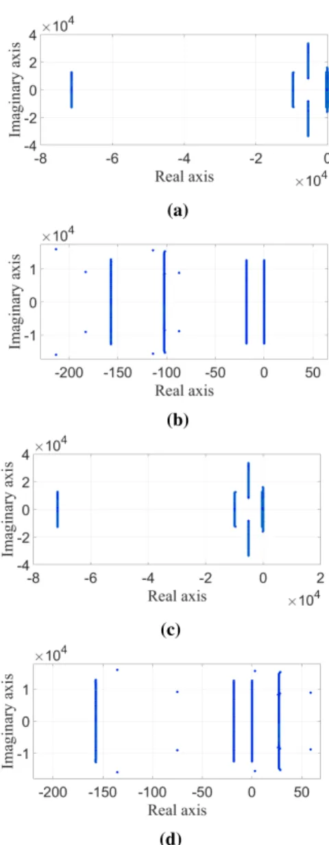
The eigenvalue loci based on the linearised model (35), with a truncation of the Toeplitz matrix at N = 40, is evaluated in order to assess the stability of the system. Referring to Table II, the continuous LTP eigenvalue loci plots are reported in Fig.3 for CASE A, where sub-figures (a)and(b)representIref =
9.4 A, which gives a stable system since all the important eigenvalues lie in the left-hand side of the complex plane, and sub-figures(c)and(d)representIref = 9.8A, which gives an unstable system, since some of the important eigenvalues lie in the right-hand side of the complex plane. Thus it can be found thatIth
ref = 9.6A. Fig.4 reports the calculatedIrefth for the set of parameters Rc ∈[0.4 : 1.6]Ω and Lg ∈[2 : 3.2]mH. The thresholds corresponding to the three cases that will be later validated experimentally have been labelled in figure. The accuracy of the stability analysis depends on the truncation order, which has been chosen based on the results presented in Fig.5, where the percentage error refers to the difference between the stability thresholds calculated using N ∈[2 : 30]
and the one using N = 100. It can be seen that forN >20
the instability thresholdIth
ref is identified with negligible error, henceN = 40has been chosen. This is due to the fact that for small N the vertical line of eigenvalues are shifted from their correct location. Some spurious eigenvalues can be seen in Fig.3. They have no physical meaning and they can be easily identified in the eigenvalue plot because they move out of the vertical lines corresponding to the translated copies of the main eigenvalues shown in Fig.2. In fact, the continuous LTP theory is based on Toeplitz forms that involve infinite harmonic terms, but the application of the truncation compromises this assumption and spurious eigenvalues arise.
From Fig.5 it can be clearly observed that the error is still acceptable, i.e. of the order of a few %, also for a truncation orderN = 8, much lower than the one used in the proposed analysis. N = 40 has been preferred in this paper only to demonstrate the potentially high precision of the method.
B. Discrete LTP Analytical Results
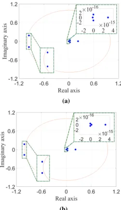
The eigenvalue loci based on the linearised model (51) is evaluated in order to assess the stability of the system. Referring to Table II, the discrete LTP eigenvalue loci plots are reported in Fig.6 for CASE A, where the first one is with Iref = 9.4 A, which gives a stable system since all the eigenvalues lie inside the unit circle, and the second one with
Iref = 9.8A, which gives an unstable system, since some of
(a)
(b)
(c)
(d)
Fig. 3. CASE A - Continuous LTP Eigenvalues: (a) stable system withIref= 9.4A, (b) zoom around the imaginary axis , (c) unstable
system withIref= 9.8A, (d) zoom around the imaginary axis.
Fig. 4. Continuous LTP: stability thresholdIrefth as function of Lg
andRc. Red lines indicate stability thresholds that will be validated
experimentally, according to Table II.
the eigenvalues lie outside of the unit circle. Thus it can be found thatIth
Fig. 5.Stability thresholdIrefth identification error as a function of the
truncation order (Threshold calculated withN = 100 is considered accurate.)
the set of parametersRc ∈[0.4 : 1.6]ΩandLg∈[2 : 3.2]mH. The thresholds corresponding to the three cases that will be later validated experimentally have been labeled in the figure.
(a)
(b)
Fig. 6.CASE A - Discrete LTP Eigenvalues: (a) stable system with
Iref = 9.4A, (b) unstable system withIref= 9.8A
C. Time-Domain Simulation Results
The simulations have been implemented in Matlab Simulink and Plecs toolbox. For brevity, only CASE A from Table II has been considered. The analysis has been performed on the switching model of the system, with control algorithm implemented in C. Moreover, the duty cycled(k)takes values in the range [−1,1], while d1(k) and d2(k) take values in the range[0,1](Fig.1), due to the modulation scheme imple-mented with a single unipolar triangular carrier of frequency
fpwmcompared compared with the two duty cycles to generate
Fig. 7. Discrete LTP: stability threshold Irefth as function of Lg
andRc. Red lines indicate stability thresholds that will be validated
experimentally, according to Table II.
the gate commands for the two legs. A double update mode is used for the PWM, and therefore the control algorithm is executed at twice the switching frequency, i.e. fx = 2fpwm. Since the IGBTs used in the experimental converter require a non negligible dead time (Tdead = 3.2 µs), a standard feed-forward compensation term is added to the signald(k), which provides a compensation to the average value of the output voltage. Such a term, sign(IL2(t))2Tdead/Tpwm, depends on the sign of the output current IL2(t) and a dead band of ±0.5A is introduced to deal with zero crossings.Vo(k)and
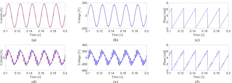
IL2(k) are acquired at discrete times kTx, while the output control signals d1(k) and d2(k) are provided by the DSP at discrete times(k+1)Tx, due to the computation delay time. In Fig.8 results of the time-domain simulation, showing converter current, capacitor voltage and phase estimated by the PLL are presented, for operation below and above the estimated stability threshold, identified asIth
ref = 9.6Aby the theoretical analysis. The small distortion that can be observed in the voltage and current waveforms in the stable case is due to the non-ideal compensation of the dead-times of the IGBTs, by the resonance of the LCL filter and by the fact that the system is operating very close to the instability boundary. It is worth noticing that in Fig. 8(d) the inductor currentIL2(t), within the
limits of the control bandwidth, correctly tracks the reference currentIref(t), confirming that the observed instability is not due to the current control but to the PLL. These simulation results provide a first validation of the accuracy of the stability boundary prediction provided by the LTP eigenvalue analysis.
D. Experimental Results
(a)
(d)
(b)
(e)
(c)
(f)
Fig. 8. Simulation results for CASE A - currents: blue -IL2(t), red -Iref(t); voltages: blue -Vo(t); phase: blue -θP LL; (a), (b), (c) stable
system withIref = 9.4A, (d), (e), (f) unstable system withIref = 9.8A.
Fig. 10. Single-phase grid-connected inverter with PLL - experi-mental setup
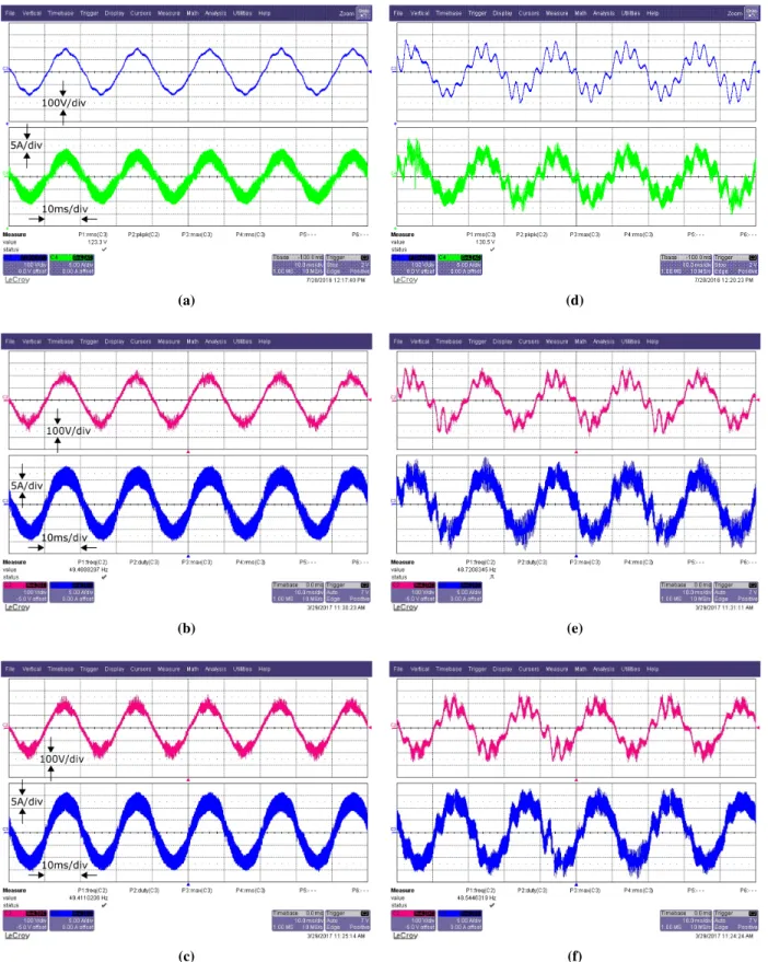
seen with the time domain simulation reported in Fig.8. In addition, Fig.11, (a) and (d), reports the converter current and capacitor voltage measured with the oscilloscope when the converter is operating below and above the threshold, with Iref = 9.4A and Iref = 9.8A respectively. The same waveforms are measured and reported in Fig.11, (b) and (e), for CASE B, with Iref = 11.3A and Iref = 11.7A, and Fig.11, (c) and (f), with Iref = 12.9A and Iref = 13.3A. A good agreement with the theoretical results presented in Fig.4 and Fig.7 can be observed.
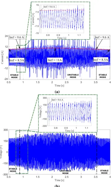
As a further validation of the threshold for CASE A, Fig.12
shows converter current and capacitor voltage, recorded by logging in Matlab the samples measured by the DSP in the ex-perimental setup, when the amplitude of the reference current
Iref changes with time following a triangular envelope with period 3.5s and minimum and maximum values respectively
8.5A and 11A. The converter current and capacitor voltage are stable for Iref <9.6A and are unstable for Iref >9.6A. The experimental results agree with the theoretical ones, corroborating the validity of the proposed stability analysis method.
VI. COMPARISON ANDDISCUSSION
From the theoretical analysis it can be seen that the con-tinuous and the discrete LTP models both enable an accurate evaluation of the stability boundaries of the system. In fact, the difference between the calculated thresholds with the two approaches is around3−4%. So the stability assessment can be accurately performed in both continuous and discrete time-domains. However, some features can be discussed as follows:
(a)
(d)
(b)
(e)
(c)
(f)
Fig. 9. Experimental results for CASE A - currents: blue -IL2(t), red -Iref(t); voltages: blue -Vo(t); phase: blue -θP LL; (a), (b), (c)
(a)
(b)
(c)
(d)
(e)
(f)
Fig. 11. CASE A - (a), stable system with Iref = 9.4A, (d), unstable system with Iref = 9.8A; CASE B - (b), stable system with
Iref = 11.3A, (e), unstable system with Iref = 11.7A; CASE C - (c), stable system with Iref = 12.9A, (f), unstable system with
Iref = 13.3A; top trace: inverter currentIL2(t), bottom trace: voltageVo(t).
• Continuous LTP: the digital computational delay plus
ZOH of the digital PWM can be approximated exploiting the Pad´e functions. No approximations are made to describe the dynamics of the grid and the filter
subsys-tem. Attention must be paid to choose a high enough truncation order, to achieve accurate results.
• Discrete LTP: the control subsystem included in the
(a)
(b)
Fig. 12.CASE A - (a) Currents: blue -IL2(t), red -Iref amplitude.
(b) Voltages: blue -Vo(t).
the digital computational delays are naturally represented in discrete time. The filter-grid continuous part must be approximated by a discrete model. No considerations related to the order of the system and truncations are required, since in this case the stability analysis relies on a different theoretical approach.
VII. CONCLUSION
In this paper a general method is presented, based on LTP theory, to perform stability analysis of power converters with non-linear control and time-periodic operating trajectories, thus providing a technique to precisely analyse single phase or heavily unbalanced three phase systems. The proposed analysis can be performed both in the continuous and in the discrete time-domain. The paper shows how the two methods, despite a different theoretical background, can identify the stability threshold with comparable precision. The objective of the analysis is to capture effects of the non-linear dynamics that would not be detectable with simplified low frequency averaging and LTI analysis. Validity of the model for high
frequencies is limited by the averaging approach employed to represent the inverter. The method has been applied to a single-phase grid-connected inverter with PLL, showing how stability depends on the amplitude of the grid current reference. For a given set of converter and grid parameters, current controller design and PLL design, with the proposed approach it is possible to derive analytically the maximum current reference that guarantees stable operation. Numerical simulations and experiments on a 10kW prototype have been performed to validate the proposed stability analysis technique, including different values of grid inductor and damping resistor, always showing a good match between the predicted stability bound-aries and those measured in the experimental setup.
REFERENCES
[1] E. Mollerstedt and B. Bernhardsson, “Out of control because of harmonics-an analysis of the harmonic response of an inverter loco-motive,”IEEE Control Systems, vol. 20, pp. 70–81, Aug 2000. [2] E. Mollerstedt and B. Bernhardsson, “A harmonic transfer function
model for a diode converter train,” inPower Engineering Society Winter Meeting, 2000. IEEE, vol. 2, pp. 957–962 vol.2, 2000.
[3] H. Liu and J. Sun, “Modeling and analysis of dc-link harmonic insta-bility in LCC HVDC systems,” in Control and Modeling for Power Electronics (COMPEL), 2013 IEEE 14th Workshop on, pp. 1–9, June 2013.
[4] M. Bollen, J. Meyer, H. Amaris, A. M. Blanco, A. G. de Castro, J. Desmet, M. Klatt, L. Kocewiak, S. R¨onnberg, and K. Yang, “Future work on harmonics - some expert opinions part I - wind and solar power,” in 2014 16th International Conference on Harmonics and Quality of Power (ICHQP), pp. 904–908, May 2014.
[5] J. Meyer, M. Bollen, H. Amaris, A. M. Blanco, A. G. de Castro, J. Desmet, M. Klatt, L. Kocewiak, S. R¨onnberg, and K. Yang, “Future work on harmonics - some expert opinions part II - supraharmonics, standards and measurements,” in 2014 16th International Conference on Harmonics and Quality of Power (ICHQP), pp. 909–913, May 2014. [6] B. Wen, D. Boroyevich, R. Burgos, P. Mattavelli, and Z. Shen, “Analysis of d-q small-signal impedance of grid-tied inverters,”IEEE Transactions on Power Electronics, vol. 31, pp. 675–687, Jan 2016.
[7] J. Sun, “Impedance-based stability criterion for grid-connected invert-ers,”IEEE Transactions on Power Electronics, vol. 26, pp. 3075–3078, Nov 2011.
[8] J. Sun and K. Karimi, “Small-signal input impedance modeling of line-frequency rectifiers,”Aerospace and Electronic Systems, IEEE Transac-tions on, vol. 44, pp. 1489–1497, Oct 2008.
[9] J. Sun, “Input impedance analysis of single-phase pfc converters,”Power Electronics, IEEE Transactions on, vol. 20, pp. 308–314, March 2005. [10] V. Salis, A. Costabeber, P. Zanchetta, and S. Cox, “A generalised har-monic linearisation method for power converters input/output impedance calculation,” in2016 18th European Conference on Power Electronics and Applications (EPE’16 ECCE Europe), pp. 1–7, Sept 2016. [11] J. Sun, “Small-signal methods for ac distributed power systems 2013; a
review,”Power Electronics, IEEE Transactions on, vol. 24, pp. 2545– 2554, Nov 2009.
[12] S. Shah and L. Parsa, “On impedance modeling of single-phase voltage source converters,” in 2016 IEEE Energy Conversion Congress and Exposition (ECCE), pp. 1–8, Sept 2016.
[13] S. Lissandron, L. D. Santa, P. Mattavelli, and B. Wen, “Experimental validation for impedance-based small-signal stability analysis of single-phase interconnected power systems with grid-feeding inverters,”IEEE Journal of Emerging and Selected Topics in Power Electronics, vol. 4, pp. 103–115, March 2016.
[14] A. G. J. MacFarlane and I. Postlethwaite, “The generalized Nyquist stability criterion and multivariable root loci,”International Journal of Control, vol. 25, no. 1, pp. 81–127, 1977.
[15] N. M. Wereley and S. R. Hall, “Frequency response of linear time periodic systems,” inDecision and Control, 1990., Proceedings of the 29th IEEE Conference on, pp. 3650–3655 vol.6, Dec 1990.
[17] J. R. C. Orillaza and A. R. Wood, “Harmonic state-space model of a controlled TCR,” IEEE Transactions on Power Delivery, vol. 28, pp. 197–205, Jan 2013.
[18] M. S. P. Hwang and A. R. Wood, “A new modelling framework for power supply networks with converter based loads and generators -the harmonic state-space,” inPower System Technology (POWERCON), 2012 IEEE International Conference on, pp. 1–6, Oct 2012.
[19] J. Kwon, X. Wang, C. L. Bak, and F. Blaabjerg, “Harmonic instability analysis of single-phase grid connected converter using harmonic state space (HSS) modeling method,” in 2015 IEEE Energy Conversion Congress and Exposition (ECCE), pp. 2421–2428, Sept 2015. [20] J. Kwon, X. Wang, C. L. Bak, and F. Blaabjerg, “Harmonic interaction
analysis in grid connected converter using harmonic state space (HSS) modeling,” in Applied Power Electronics Conference and Exposition (APEC), 2015 IEEE, pp. 1779–1786, March 2015.
[21] R. Z. Scapini, L. V. Bellinaso, and L. Michels, “Stability analysis of half-bridge rectifier employing LTP approach,” inIECON 2012 - 38th Annual Conference on IEEE Industrial Electronics Society, pp. 780–785, Oct 2012.
[22] L. V. Bellinaso, R. Z. Scapini, and L. Michels, “Modeling and analysis of single phase full-bridge PFC boost rectifier using the LTP approach,” inXI Brazilian Power Electronics Conference, pp. 93–100, Sept 2011. [23] C. Zou, B. Liu, S. Duan, and R. Li, “Influence of delay on system stability and delay optimization of grid-connected inverters with lcl filter,”IEEE Transactions on Industrial Informatics, vol. 10, pp. 1775– 1784, Aug 2014.
[24] C. Zhang, X. Wang, and F. Blaabjerg, “Analysis of phase-locked loop influence on the stability of single-phase grid-connected inverter,” in
2015 IEEE 6th International Symposium on Power Electronics for Distributed Generation Systems (PEDG), pp. 1–8, June 2015. [25] V. Salis, A. Costabeber, P. Zanchetta, and S. Cox, “Stability analysis of
single-phase grid-feeding inverters with pll using harmonic linearisation and linear time periodic (ltp) theory,” in2016 IEEE 17th Workshop on Control and Modeling for Power Electronics (COMPEL), pp. 1–7, June 2016.
[26] D. M. Van de Sype, K. De Gusseme, A. P. Van den Bossche, and J. A. Melkebeek, “Small-signal Laplace-domain analysis of uniformly-sampled pulse-width modulators,” inPower Electronics Specialists Con-ference, 2004. PESC 04. 2004 IEEE 35th Annual, vol. 6, pp. 4292–4298 Vol.6, June 2004.
[27] S. Buso and P. Mattavelli, Digital Control in Power Electronics, 2nd Edition. Morgan & Claypool, 2015.
[28] R. Meyer and C. Burrus, “A unified analysis of multirate and periodically time-varying digital filters,”IEEE Transactions on Circuits and Systems, vol. 22, pp. 162–168, Mar 1975.
[29] S. Bittanti and P. Colaneri, “Invariant representations of discrete-time periodic systems,”Automatica, vol. 36, no. 12, pp. 1777 – 1793, 2000. [30] Z. Bing, K. Karimi, and J. Sun, “Input impedance modeling and analysis of line-commutated rectifiers,”Power Electronics, IEEE Transactions on, vol. 24, pp. 2338–2346, Oct 2009.
Valerio Salisreceived the Master’s degree with hon-ours in Electronic Engineering from the University of Rome Tor Vergata, Rome, Italy, in 2014. He is currently working towards the Ph.D. degree in Electrical and Electronic Engineering in the Power Electronics, Machines and Control Group, Univer-sity of Nottingham, Nottingham, UK. His research interests include study of instability issues in mi-crogrids, linear time periodic system analysis and control design.
Alessandro Costabeber(S’09 - M’13) received the Degree with honours in Electronic Engineering from the University of Padova, Padova, Italy, in 2008 and the Ph.D. in Information Engineering from the same university in 2012, on energy efficient architectures and control techniques for the development of future residential microgrids. In the same year he started a two-year research fellowship with the same univer-sity. In 2014 he joined the PEMC group, Department of Electrical and Electronic Engineering, University of Nottingham, Nottingham, UK as Lecturer in Power Electronics. His current research interests include HVDC converters topologies, high power density converters for aerospace applications, control solutions and stability analysis of AC and DC microgrids, control and modelling of power converters, power electronics and control for distributed and renewable energy sources. Dr. Costabeber received the IEEE Joseph John Suozzi INTELEC Fellowship Award in Power Electronics in 2011.
Stephen M. Coxreceived the B.A. degree in mathe-matics from the University of Oxford, Oxford, U.K., in 1986, and the Ph.D. degree in applied mathemat-ics from the University of Bristol, Bristol, U.K., in 1989. He is currently a Reader in the School of Mathematical Sciences, University of Nottingham, Nottingham, U.K., where he was also a Lecturer and then a Senior Lecturer. From 2004 to 2006, he was a Senior Lecturer in the School of Mathematical Sciences, University of Adelaide, Australia. His re-search interests include the development of applied mathematical techniques for the modeling of class-D amplifiers and other power-electronic switching devices.
Pericle Zanchetta (M’00 - SM’15) received his MEng degree in Electronic Engineering and his Ph.D. in Electrical Engineering from the Technical University of Bari (Italy) in 1993 and 1997 respec-tively. In 1998 he became Assistant Professor of Power Electronics at the same University. In 2001 he became lecturer in control of power electronics systems in the PEMC research group at the Univer-sity of Nottingham UK, where he is now Professor in Control of Power Electronics systems. He has published over 260 peer reviewed papers and he is Chair of the IAS Industrial Power Converter Committee IPCC. His research interests include control of power converters and drives, Matrix and multilevel converters.